Deriving Quantitative Crystallographic Information from the Wavelength-Resolved Neutron Transmission Analysis Performed in Imaging Mode


Faculty of Engineering, Hokkaido University, Kita-13 Nishi-8, Kita-ku, Sapporo, Hokkaido 060-8628, Japan
J. Imaging 2018, 4(1), 7; https://doi.org/10.3390/jimaging4010007
Submission received: 25 November 2017
/
Revised: 18 December 2017
/
Accepted: 20 December 2017
/
Published: 28 December 2017
(This article belongs to the Special Issue Neutron Imaging)
Abstract
:Current status of Bragg-edge/dip neutron transmission analysis/imaging methods is presented. The method can visualize real-space distributions of bulk crystallographic information in a crystalline material over a large area (~10 cm) with high spatial resolution (~100 μm). Furthermore, by using suitable spectrum analysis methods for wavelength-dependent neutron transmission data, quantitative visualization of the crystallographic information can be achieved. For example, crystallographic texture imaging, crystallite size imaging and crystalline phase imaging with texture/extinction corrections are carried out by the Rietveld-type (wide wavelength bandwidth) profile fitting analysis code, RITS (Rietveld Imaging of Transmission Spectra). By using the single Bragg-edge analysis mode of RITS, evaluations of crystal lattice plane spacing (d-spacing) relating to macro-strain and d-spacing distribution’s FWHM (full width at half maximum) relating to micro-strain can be achieved. Macro-strain tomography is performed by a new conceptual CT (computed tomography) image reconstruction algorithm, the tensor CT method. Crystalline grains and their orientations are visualized by a fast determination method of grain orientation for Bragg-dip neutron transmission spectrum. In this paper, these imaging examples with the spectrum analysis methods and the reliabilities evaluated by optical/electron microscope and X-ray/neutron diffraction, are presented. In addition, the status at compact accelerator driven pulsed neutron sources is also presented.
1. Introduction
Wavelength-resolved neutron transmission imaging experiments using the time-of-flight (TOF) method at pulsed cold/thermal neutron sources can position-dependently obtain Bragg-edge transmission spectra from a polycrystalline material, or Bragg-dip transmission spectra from a coarse-grained/single-crystal material, at each pixel position of a neutron TOF-imaging detector. Bragg-edge is the profile caused by diffraction phenomenon of neutrons in a polycrystal and Bragg-dip is the profile caused by diffraction phenomenon of neutrons in a single-crystal. Therefore, these profiles include crystallographic information of each crystal. Bragg-edge transmission spectrum includes bulk crystallographic information averaged over a neutron transmission path in a polycrystalline material, e.g., quantities of each crystalline phase, degree of crystallographic anisotropy (texture), preferred orientation, crystallite size, crystal lattice plane spacing (d-spacing) relating to macro-strain, d-spacing distribution’s broadening relating to micro-strain (relating to dislocation density etc.) of each phase. Bragg-dip transmission spectrum includes bulk crystallographic information along a neutron transmission path in a coarse-grained/single-crystal material, e.g., the number of crystalline grains, crystal orientations of each grain and so on. Additionally, this microstructural information can be mapped over a large area (~10 cm × 10 cm) with high spatial resolution (~100 μm) owing to neutron imaging detectors. It is not so easy for conventional methods such as SEM-EBSD (scanning electron microscopy-electron backscatter diffraction), X-ray diffraction/tomography and neutron diffraction to achieve these advantages at the same time: e.g., the presented method has the simultaneous 2D/3D imaging capability for bulk crystallographic information without the beam scanning, which is not easy even for neutron diffractometers. For this reason, various Bragg-edge/dip transmission imaging techniques have been developed recently.
In this paper, present status of quantitative evaluation/imaging methods for these crystallographic information is presented. For the quantitative evaluation, the profile analysis of Bragg-edge/dip transmission spectra is quite important. For this reason, in Section 2, the spectrum profile analysis methods are presented. Examples of quantitative imaging of texture/crystallite-size, crystalline phase and crystal lattice strain are presented in Section 3, Section 4 and Section 5, respectively. The quantification performances checked by neutron diffraction etc. are also presented. In Section 6, the development status of quantitative macro-strain tomography technique based on the Bragg-edge transmission method is introduced. Examples of quantitative imaging of grain orientation are presented in Section 7.
2. Bragg-Edge/Dip Profile Analysis for Quantitative Evaluation of Crystalline Microstructural Information
2.1. Information Included in Bragg-Edge/Dip Neutron Transmission Spectrum
Figure 1a shows examples of Bragg-edge neutron transmission spectrum and the included information and Figure 1b shows an example of Bragg-dip neutron transmission spectrum and the included information. Both the wavelength-dependent neutron transmission spectra mainly reflect neutron attenuation based on the Bragg’s law (diffraction):
Here, λ is neutron wavelength, dhkl is crystal lattice plane spacing (d-spacing) of the crystal lattice plane {hkl} and θhkl is Bragg angle for the crystal lattice plane {hkl}. Wavelength-resolved neutron transmission imaging experiments use polychromatic neutrons, while the wavelengths are analysed by the TOF method etc. Therefore, neutrons in a polycrystalline material can be diffracted at various wavelengths from λ = 2dhklsin0° to λ = 2dhklsin90° and there are no diffracted neutrons at λ > 2dhklsin90°. As a result, Bragg-edge appears at λ = 2dhkl. Thus, dhkl can be deduced from the Bragg-edge wavelength λ = 2dhkl. In addition, the elastic macro-strain ε in crystal lattice can be evaluated by:
Here, d0 is d-spacing without strain/stress. At the same time, broadening of the dhkl distribution relating to micro-strain (relating to dislocation density etc.) can be deduced from broadening of Bragg-edge.
At the wavelength λ < 2dhkl, the wavelength-dependent intensity reflects the angle-dependent intensity of diffracted neutrons, according to Equation (1) which indicates the relation between λ and θhkl. In other words, crystallographic anisotropy (orientation distribution) and preferred orientation due to texture can be evaluated from shape of wavelength-dependent transmission spectrum. The intensity increase caused by multiple diffraction due to the primary extinction effect inside a crystallite reflects the crystallite size. Of course, the whole Bragg-edge pattern reflects the number of crystalline phases and the crystal structure of each phase.
On the other hand, neutrons in a single-crystal/coarse-grained material can be diffracted in certain wavelengths because diffraction occurs only in a certain Bragg angle. As a result, Bragg-dip appears at λ = 2dhklsinθhkl (θhkl can be changed depending on the crystal orientation of a grain). Thus, the number of grains and the crystal orientation of each grain can be deduced from the Bragg-dip pattern.
2.2. Profile Calculation Model for Bragg-Edge Transmission Spectrum Analysis: Algorithm of the RITS Code
For the Bragg-edge transmission analysis and the crystallographic information evaluation, the RITS (Rietveld Imaging of Transmission Spectra) code was developed and checked by neutron diffraction etc. [1,2,3,4,5,6,7,8,9]. RITS is based on the idea of the Rietveld analysis method [10] for X-ray/neutron powder diffractometry. Firstly, RITS calculates a neutron transmission spectrum based on theoretical crystalline microstructural models. Then, RITS fits it to experimental data of transmission spectrum by using the nonlinear least-squares fitting algorithm, the Levenberg-Marquardt method [11]. Thus, RITS can refine the crystalline microstructural models which can well reconstruct the experimental data of transmission spectrum. The three important features of the RITS code are:
- Automatic calculation function for multiple elements, multiple crystalline phases and 230 crystal structure space groups [5].
In this section, the crystalline microstructural models used in RITS are presented.
2.2.1. Neutron Transmission and Total Cross-Section
Wavelength-dependent neutron transmission rate (neutron transmission spectrum) Tr(λ) is experimentally measured as the ratio of wavelength-dependent neutron counts transmitted through a sample I(λ) to wavelength-dependent neutron counts without the sample I0(λ) as follows:
Note that I(λ) and I0(λ) do not contain the background noise. On the other hand, Tr(λ) is theoretically expressed by:
where p is index of crystalline phase, σtot is total cross-section, ρ is atomic number density and t is thickness, respectively. Note that the projected atomic number density ρt can be evaluated in a transmission spectroscopy. By using the refined projected atomic number density ρt, the volume fractions of each crystalline phase can be deduced and mapped [9].
The total cross-section consists of components of coherent elastic scattering, incoherent elastic scattering, inelastic scattering and absorption and can be written by:
The coherent elastic scattering mainly consists of nuclear Bragg scattering and RITS calculates this component for quantitative evaluation of crystallographic information. Incidentally, note that there are also small portions of magnetic Bragg scattering component [12,13] and small-angle scattering component [14,15] in the coherent elastic scattering, actually.
In the RITS code, the calculation algorithm of the incoherent elastic scattering and the inelastic scattering is based on Granada’s model [16] and the calculation algorithm of the absorption is based on so-called the 1/v law. These models were adopted in the CRIPO code [17] and the BETMAn code [18], which were pioneer codes before the RITS code and also in the NXS code [19] which was a calculation code developed in 2012.
2.2.2. Coherent Elastic Scattering (Nuclear Bragg Scattering) and the Crystal Structure Factor
The coherent elastic scattering expression in the RITS code [1] is described by:
This is based on the Fermi’s kinematical model [20], the Jorgensen-type edge profile function Rhkl(λ) [18,21,22] for strain analysis, the March-Dollase preferred orientation function Phkl(λ) [18,22,23] for texture analysis and Sabine’s primary extinction function Ehkl(λ) [22,24,25] for crystallite size analysis. Here, V0 is unit cell volume of crystal structure and Fhkl is the crystal structure factor that is defined by the same definition of crystallography [7]:
where n expresses index of atoms in the crystal structure, on is site occupancy of nth atom, bn is scattering length of nth atom, (xn, yn, zn) is fractional coordinate of nth atom, the exponential is the Debye-Waller factor and Biso is isotropic atomic displacement parameter, respectively.
2.2.3. Edge Profile Function Rhkl(λ) for Macro/Micro-Strain Correction/Analysis
The edge profile function used in the RITS code, Rhkl(λ), is the Jorgensen-type edge profile function [18,21,22]. This function can describe the profile change near Bragg-edge due to instrumental wavelength resolution and micro-strain (relating to dislocation density etc.). The expression [4] is:
where
and
Here, σhkl is a broadening parameter representing the Bragg-edge profile. In the RITS code, this parameter is separated to the instrumental wavelength resolution part σ0 (the standard deviation of (asymmetric) Jorgensen-type edge profile function) and the micro-strain part σ1’ (the standard deviation of (symmetric) complementary error function), respectively [6]:
and
σ1’,hkl represents the standard deviation and whkl represents FWHM (full width at half maximum) of the d-spacing distribution expressed by the Gaussian profile. Moreover, αhkl is the rising parameter of Bragg-edge and βhkl is the decaying parameter of Bragg-edge. By determining the instrumental wavelength resolution parameters σ0,hkl, αhkl and βhkl before material characterization, the micro-strain parameter σ1’,hkl (whkl) of a specimen can be evaluated from the Bragg-edge profile [6].
Through the Bragg-edge profile analysis using the single Bragg-edge analysis mode of the RITS code, dhkl can be evaluated, as well as pioneer works [26,27] using the Kropff-type edge profile function which is simpler than the Jorgensen-type, without the distortion due to micro-strain effect [4,6]. It is also a feature of RITS that whkl can be also evaluated at the same time. In the single Bragg-edge analysis mode of the RITS code, three-stage fitting method [26] is adopted for easy and accurate profile fitting. Note that the three-stage fitting method is a step-by-step fitting algorithm for spectrum of three wavelength regions before/around/after a Bragg-edge. The data-analysis examples are described in Section 5 and Section 6.
2.2.4. March-Dollase Type Preferred Orientation Function Phkl(λ) for Crystallographic Texture Correction/Analysis
The preferred orientation function used in the RITS code, Phkl(λ), is the March-Dollase function for all θhkl [18,22]. This function can describe the shape change over whole transmission spectrum due to preferred orientation and degree of crystallographic anisotropy. The expression [1] is:
where
and
Ohkl(α,β) corresponds to so-called the pole figure of {hkl} with the latitude angle (= Bragg angle) α and the longitude angle β. The function inside the integral of Equation (16) is the March function. In other words, in the March-Dollase model, the pole figure is described by the March model. In addition, Equation (16) represents that α (Bragg angle θhkl) dependent orientation distribution is observable but the distribution is integrated and averaged over all β; β-dependent orientation distribution is not observable in the Bragg-edge transmission spectroscopy. A of Equation (18) represents angle between the plane-normal vector of considering diffraction <hkl> and the preferred orientation vector <HKL>.
By using this function, two kinds of information about crystallographic texture can be evaluated. One is the degree of crystallographic anisotropy, the March-Dollase coefficient R. If R is equal to 1, Phkl(λ) is 1 that represents no texture (isotropic orientation distribution). If R is close to 0 or ∞, strong texture exists in a specimen (anisotropic orientation distribution). The other is the preferred orientation vector <HKL>. When R is less than 1, <HKL> represents the preferred orientation parallel to the neutron incident/transmission direction (α = θhkl = 90° direction). When R is greater than 1, <HKL> represents the preferred orientation perpendicular to the neutron incident/transmission direction (α = θhkl = 0° direction). The data-analysis examples are described in Section 3 and Section 4.
2.2.5. Sabine’s Primary Extinction Correction Function Ehkl(λ) for Crystallite Size Analysis
The primary extinction correction/analysis function used in the RITS code, Ehkl(λ), is Sabine’s function [22,24,25]. This function can describe the intensity increase over whole transmission spectrum (decrease of diffraction intensity) due to multiple diffraction of neutrons inside a crystallite. Thus, this effect can reflect the size of crystallite. The expression [1] is:
where
and
Here, S is the size of crystallite (cubic shape). If S is zero, Ehkl(λ) is 1 (no extinction). If S becomes larger, Ehkl(λ) becomes smaller (extinction becomes stronger, total cross-section becomes smaller and transmission intensity becomes larger). The data-analysis examples are described in Section 3 and Section 4.
2.3. Bragg-Dip Pattern Analysis Method
Hereafter, a grain orientation analysis/imaging method using the Bragg-dip neutron transmission spectrum [28] is presented. Although detailed crystallographic characterization of a single-crystal material can be performed by whole pattern fitting analysis toward Bragg-dip transmission spectrum [29,30], the author considered that the Bragg-dip neutron transmission method also becomes a useful method for grain orientation imaging as well as neutron diffraction imaging techniques [31,32]. Since a fast determination method of the number of grains and their crystal orientations from a Bragg-dip pattern is developed for this aim, the data analysis procedure is briefly presented in this section; the details are reported in [28].
2.3.1. Database Matching Method for Fast Determination of the Number of Crystalline Grains and Their Crystal Orientations
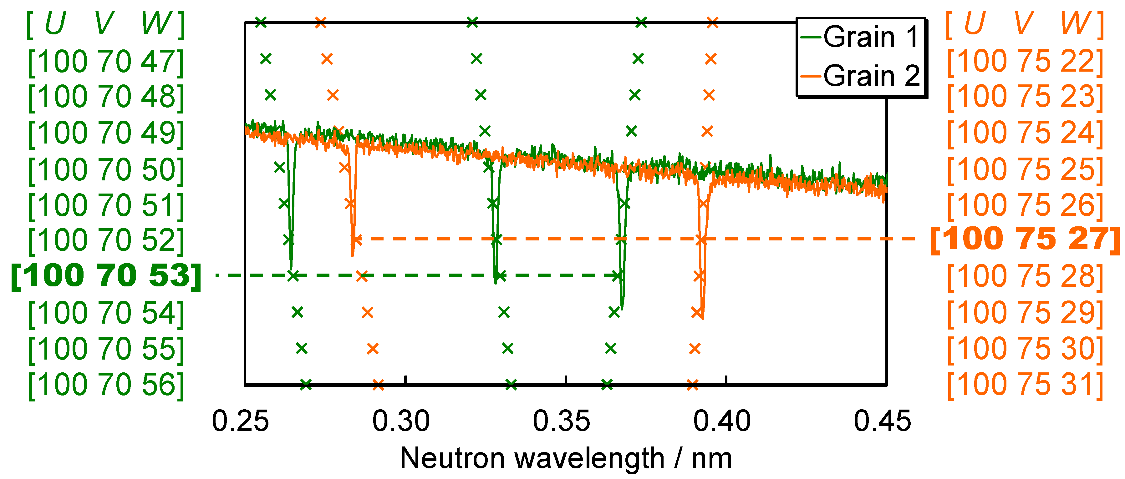
Figure 2 shows a scheme of the developed grain-orientation determination method, the database matching method. First of all, appearing wavelengths of Bragg-dips are evaluated from the experimental data. Next, the crystal orientation [UVW] parallel to the neutron incident/transmission direction is determined. For this determination, a suitable pattern which can reconstruct the experimental Bragg-dip pattern is uniquely searched from the database. The database contains Bragg-dip wavelength patterns of all <UVW>. Angle between the normal vector [hkl] of a possible diffraction plane (hkl) and a certain crystal-lattice direction parallel to neutron beam [UVW] is calculated by:
In this case, the Bragg angle of the (hkl) diffraction is
Finally, the wavelength where (hkl) Bragg-dip appears is calculated from Equations (1) and (26). This procedure is repeated about all possible (hkl) and the wavelength pattern is recorded for each [UVW] case. Thus, the database about Bragg-dip wavelength pattern for all [UVW] can be made.
Through matching between experimental pattern and calculated pattern, [UVW] of single crystal (grain) of the experimental data can be uniquely deduced. Features of this method are:
- Fast determination of crystal orientation without any initial estimation.
- Data obtained from multiple grains can be analysed. In this case, the number of grains and their crystal orientations are individually determined. (Of course, there is a limit of acceptable number).
However, it is not so easy for this method to evaluate a material of unknown crystal structure or multiple crystalline phases.
2.3.2. Validity of Evaluated Crystal Orientation
Figure 3 shows two examples of Bragg-dip transmission data and the database matching result (cross × marks) with the information of indexing (hkl) [28]. The single-crystal sample was 3.4 wt % Si-steel plate of 5 mm thickness and was measured at a pulsed cold-neutron beam-line, BL10 “NOBORU” [33] of the Materials and Life Science Experimental Facility (MLF) at the Japan Proton Accelerator Research Complex (J-PARC). The cold neutron wavelength resolution was about 0.35% and the beam angular divergence was about 416 μrad (the collimator ratio (L/D) was about 2400). The database matching was applied to the wavelength region above 0.25 nm although cross × marks and indexing results were also indicated outside the matching wavelength region in Figure 3. The crystal-lattice direction parallel to the neutron beam direction [UVW] was estimated as [100 30 8] for Grain Orientation 1 and was estimated as [100 38 0] for Grain Orientation 2, respectively. Note that evaluated crystal orientations are reasonable according to SEM-EBSD [28].
This figure indicates that a certain Bragg-dip pattern contained in the database is well matched. In addition, about Grain Orientation 2, the Bragg-dip at 0.213 nm becomes deeper and the Bragg-dip at 0.268 nm becomes deepest. The indexing result can evaluate that the deeper Bragg-dip at 0.213 nm is caused by double stacking of (211) and (21-1) Bragg-dips and the deepest Bragg-dip at 0.268 nm is caused by triple stacking of (200), (101) and (10-1) Bragg-dips although the dip depth was not analysed. Thus, it is concluded that the reliability of the developed database matching method is reasonable, checked by EBSD and the relation between indexing and dip depth.
3. Texture and Crystallite-Size Imaging by Rietveld-Type Bragg-Edge Analysis
By using the Rietveld-type (wide wavelength bandwidth) analysis of the RITS code, two-dimensional distribution of crystalline phase, texture and crystallite-size bulk-averaged along neutron transmission path in a material can be quantitatively mapped. In this section, the first example of quantitative imaging of texture and crystallite-size is presented with the results checked by neutron diffraction Rietveld analysis [1,2].
3.1. Experimental
Figure 4 shows a photograph of specimens. The measured samples were rolled α-iron plates (JIS-SS400) of 6 mm thickness along the neutron transmission direction. There are three types of samples:
- Two rolled plates (Samples A and B in Figure 4). Relation between neutron transmission direction and rolling direction are perpendicular.
- Welded plate (Sample D in Figure 4). Relation between neutron transmission direction and rolling direction are perpendicular. (Relation between neutron transmission direction and normal direction (ND) are parallel.)
- Welded plate (Sample C in Figure 4). Relation between neutron transmission direction and rolling direction (RD) are parallel.
It was well known that the preferred orientation parallel to the rolling direction of α-iron plate is <110> and the preferred orientation perpendicular to the rolling direction of α-iron plate is <111> [34]. In this experiment, it was investigated whether the Bragg-edge transmission imaging with the RITS code can identify the correct preferred orientation. In addition, changes of the degree of crystallographic anisotropy and the crystallite size between rolled plate and welded plate were quantitatively visualized.
The pulsed neutron transmission imaging experiment was performed at a cold neutron beam-line connected to a coupled-type 20 K solid CH4 moderator installed at the Hokkaido University Neutron Source (HUNS) [35,36] in Japan. HUNS is a pulsed neutron experimental facility based on 1.2 kW electron LINAC, which is one of compact accelerator driven neutron sources [37]. The distance from the neutron source to the sample/detector position was about 6 m. The maximum neutron flux is less than 104 n/cm2/s and the cold-neutron wavelength resolution of the TOF method is about 3% due to the coupled moderator and the short neutron flight distance. The collimator ratio (L/D) is 60 (beam angular divergence of 16.6 mrad).
The used neutron TOF-imaging detector was 10B-type GEM (gas electron multiplier) detector developed by Prof. Uno of High Energy Accelerator Research Organization (KEK) [38]. The GEM detector has the pixel size of 800 μm and the detection area is 10.24 cm × 10.24 cm. By using this detector, samples shown in Figure 4 were simultaneously measured. The measurement time were 5.0 hours for sample beam and 3.3 hours for open beam, respectively.
3.2. Spectrum Fitting Analysis Results
Figure 5 shows measured Bragg-edge transmission spectra and the fitting curves obtained by the RITS code, at RD rolled area, ND rolled area and ND welded area. Note that Bragg-edge transmission spectrum of RD welded area almost corresponded to the spectrum of ND welded area. Firstly, shape of transmission spectrum is changed and depends on positions. As described before, the shape change of transmission spectrum reflects variation of texture evolution or preferred orientation. For example, {110} Bragg-edge of the RD rolled area becomes peak-like near the Bragg-edge wavelength (0.405 nm). This means orientation distribution has a peak near θ110 = 90°. In other words, <110> faces to the neutron incident/transmission direction, namely, the preferred orientation parallel to the beam direction at the RD rolled area is <110>. This is consistent with the well-known preferred orientation of rolling textures [34]. On the other hand, at the ND rolled area, {110} Bragg-edge transmission intensity has a valley near λ = 0.35 nm (θ110 = 60°). This means <110> faces to the direction near θ110 = 60° and the other preferred orientation exists along the beam direction. According to the RITS analysis, this preferred orientation was estimated as <111> [1]. This is also consistent with the well-known preferred orientation of rolling textures [34]. Since the transmission shape of welded zones is close to ideal Bragg-edge transmission spectrum shape, it is estimated that there are weak texture at welded zones.
In addition, the transmission intensity of welded zones is quite lower than that of as-rolled zones. This means the crystallite size becomes smaller at welded zones (the extinction effect becomes small).
3.3. Imaging Results
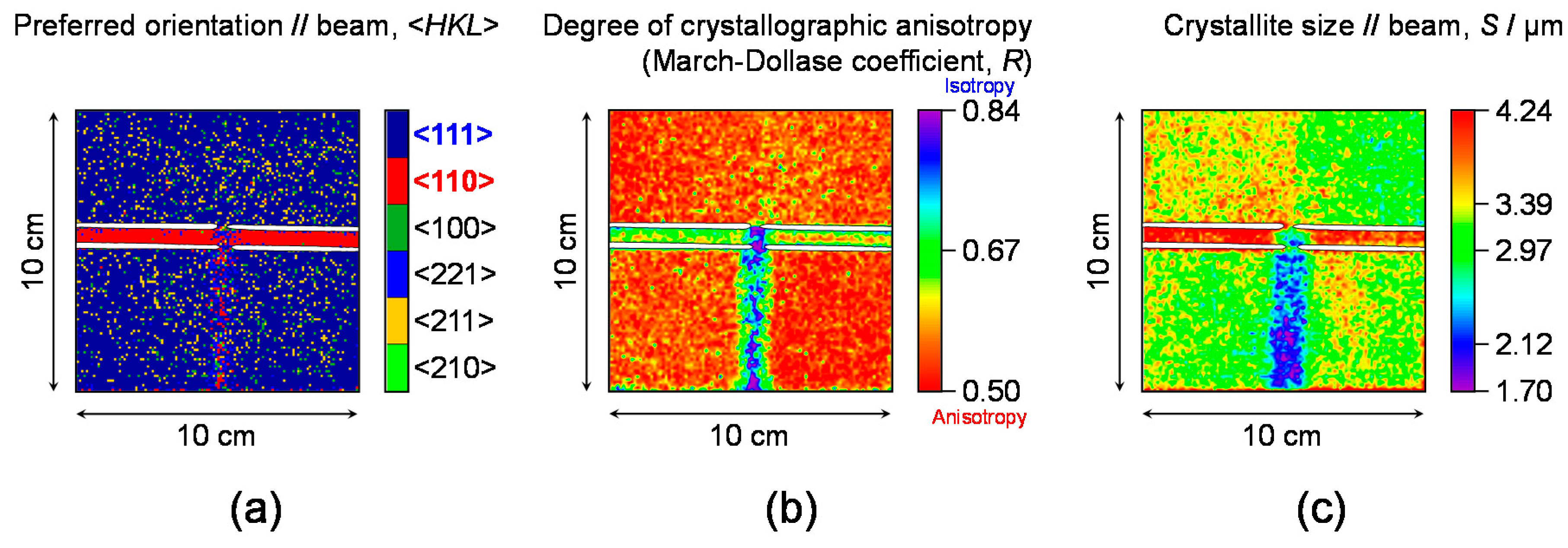
The analyses using the RITS code were performed at each pixel of the imaging detector. Figure 6 shows quantitative imaging results of (a) preferred orientation <HKL> parallel to neutron transmission direction, (b) March-Dollase coefficient R indicating degree of crystallographic anisotropy and (c) crystallite size S [1]. According to Figure 6a, it is clearly visualized that the preferred orientation parallel to ND is <111> and the preferred orientation parallel to RD is <110>, respectively. These are consistent with the theory of rolling deformation textures [34]. According to Figure 6b, it is clearly visualized that the degree of crystallographic anisotropy is changed between rolled zone and welded zone. The degree of anisotropy at the welded (center) zones of Sample C and Sample D becomes weaker than that at the as-prepared zones. It is also confirmed by Figure 6a; a certain preferred orientation is not identified at the welded zones. This means welding causes recrystallization by melting. According to Figure 6c, it is clearly visualized that the crystallite size is changed between Sample A and Sample B and between rolled zone and welded zone. The crystallite size at the welded (center) zones of Sample C and Sample D becomes smaller than that at the as-prepared zones. This means fast recrystallization after welding causes fine microstructures. Thus, bulk texture and microstructure information can be quantitatively visualized.
3.4. Check by Optical Microscope and Neutron Diffraction
The results about four conditions in these samples, roll ND data, roll RD data, weld ND data and weld RD data, were compared with the results of the Rietveld analyses of neutron diffraction data [2]. The neutron diffraction experiments were performed at J-PARC MLF BL20 “iMATERIA” [39] and the used Rietveld analysis code was Z-Rietveld [40] developed by High Energy Accelerator Research Organization (KEK). Figure 7 shows the comparison results of (a) the March-Dollase coefficient R and (b) the crystallite size S between both methods [2,7,36]. The March-Dollase coefficients are consistent within the error bars and the crystallite sizes evaluated by Bragg-edge transmission method are just 110% of the values evaluated by neutron diffraction Rietveld analysis. (Incidentally, it is estimated that reason of this 10% difference is the low wavelength resolution of HUNS [41]). In addition, it was also confirmed that the evaluated crystallite sizes were proportional to the grain sizes observed by optical microscope [1]. Thus, the reliability of the texture and crystallite-size analysis method of Bragg-edge transmission imaging using the RITS code was confirmed.
4. Crystalline Phase Imaging with Texture/Extinction Corrections
Some previous works [42,43] achieved tomographic imaging of crystalline phases at intense pulsed spallation source and reactor source. On the other hand, since the RITS code has correction functions for texture effect and extinction effect as mentioned in Section 2.2, more correct crystalline phase evaluation is expected. In this section, the latest crystalline phase imaging using the RITS code, performed at a compact accelerator driven pulsed neutron source, [44] is partially presented.
4.1. Experimental
Figure 8 shows a photograph of the sample. The sample was a knife composed of ferrite (α-Fe, body centered cubic (BCC) crystal structure) phase and austenite (γ-Fe, face centered cubic (FCC) crystal structure) phase. Although it was confirmed by X-ray diffraction experiments that two phases exist in this sample, the real-space distributions were not clear. For this reason, distributions of crystalline phases in this sample were investigated by Bragg-edge neutron transmission imaging.
The experiment was performed at HUNS. The experimental conditions are almost same as those described in Section 3.1. The used neutron TOF-imaging detector was a high-speed CMOS camera (developed by NAC Image Technology) coupled to the neutron color image intensifier (developed by TOSHIBA), integrated by Prof. Mochiki of Tokyo City University [44]. The detector was used in the mode of 66 μs TOF bin width, 13.3 cm × 13.3 cm field-of-view and 520 μm pixel size. The measurement time were 15 hours for sample beam and 12 hours for open beam, respectively.
4.2. Spectrum Fitting Analysis Result
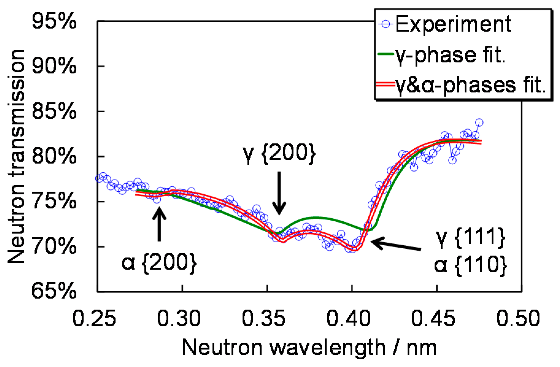
Figure 9 shows an example of measured Bragg-edge transmission spectrum with the fitting curves obtained by RITS. Since the coupled moderator and the short neutron flight path length were utilized, broad Bragg-edges were observed. Namely, Bragg-edges of α-Fe and γ-Fe were not clearly identified. However, the wide-wavelength-bandwidth curve fitting using the RITS code considering the instrumental wavelength resolution of HUNS well reconstructed the experimental data and gave the information that two crystalline phases (α-Fe and γ-Fe) were included in the sample because the curve of two-phase assumption was more suitable than the curve of one-phase assumption. Thus, the whole pattern fitting analysis function of the RITS code is useful for not only texture/extinction corrections but also low wavelength resolution case.
4.3. Imaging Results
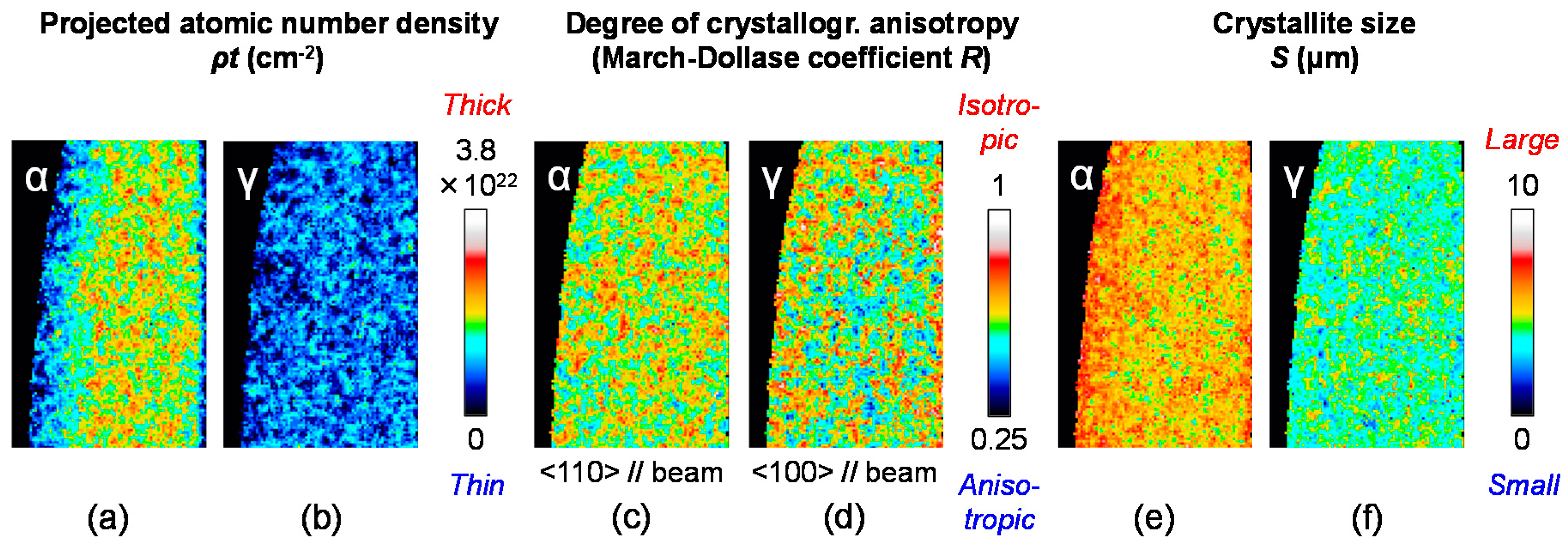
The analyses using the RITS code were performed at each pixel of the imaging detector. Figure 10a,b show imaging results of projected atomic number density ρt of each phase (see Equation (4)). Figure 10c–f show the March-Dollase coefficient (degree of crystallographic anisotropy) and the crystallite size of each phase. (Note that the statistical precisions of the images will be improved at large pulsed neutron experimental facilities.) It is interesting that textures and microstructures of each phase are not spatially changed: it is quite different from Japanese swords [45]. Namely, this knife sample has not received heat treatment such as quenching and plastic deformation such as strain hardening. On the other hand, according to Figure 10a,b, soft BCC phase exists the whole region but decreases near the cutting edge. Hard FCC phase relatively increases near the cutting edge but thin. Thus, it was concluded by Bragg-edge neutron transmission imaging that this knife had composite structure of soft ferrite and hard austenite, and was made without heat treatment (quenching) and plastic deformation (strain hardening).
4.4. Check by Neutron Diffraction
According to a Bragg-edge transmission imaging experiment with the RITS code and a neutron diffraction experiment with the Z-Rietveld code performed at J-PARC, Su et al. investigated that the volume fraction analyses between martensite phase (α’-Fe) and austenite phase (γ-Fe) could be successfully conducted by the RITS code over wide range of the phase ratio (see [9]). In addition, more detailed checking at various instruments and various (texture and extinction) correction conditions is also in progress [41].
5. Imaging of Crystal Lattice Plane Spacing (Macro-Strain) and Its Distribution’s Broadening (Micro-Strain)
The first Bragg-edge transmission imaging of macro-strain (see Equation (2)) was demonstrated at the ISIS pulsed spallation neutron experimental facility at Rutherford Appleton Laboratory in UK [27]. On the other hand, in this section, simultaneous imaging of macro-strain and micro-strain [6] and the comparisons between Bragg-edge neutron transmission and neutron diffraction [3,8] are presented.
5.1. Experimental
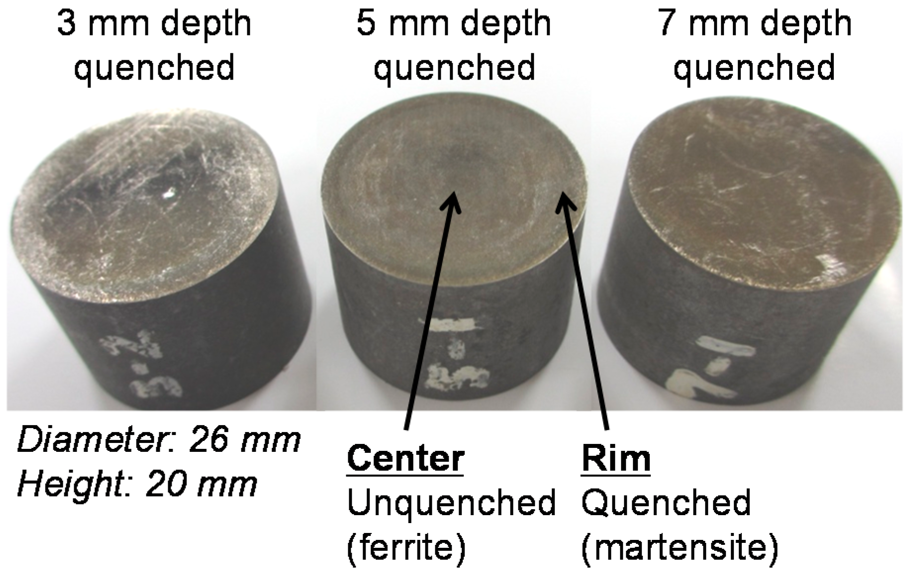
Figure 11 shows a photograph of samples. The samples were three types of ferritic steel rod (JIS-S45C) quenched by induction hardening. The samples are similar to crankshafts in an automotive. The dimensions were 2.0 cm in height and 2.6 cm in diameter. The neutron beam was transmitted along the axial direction. From the outer rim surface, quenching was treated. The aimed quenched depth were 3 mm, 5 mm and 7 mm, respectively. At the quenched zone (the rim region), the martensite phase (BCT (body centered tetragonal) crystal structure) was produced. On the other hand, ferrite phase remains at the center region. Since the interesting relation between the broadening of crystal lattice plane spacing distribution (relating to micro-strain) and the Vickers hardness was investigated by Bragg-edge transmission imaging, the results are presented here.
The experiment was performed at J-PARC MLF BL10 “NOBORU” [33] connected to decoupled-type 20 K supercritical para-H2 moderator. The accelerator power of the proton synchrotron was 120 kW during this experiment. L/D was 337 (the beam angular divergence was 3 mrad) due to collimator setup in the beam-line and the estimated cold neutron flux was about 106 n/cm2/s. The cold-neutron wavelength resolution was about 0.35%. The neutron flight path length from the moderator to the detector was about 14 m. The used neutron TOF-imaging detector was 10B-MCP (micro channel plate) type detector developed by Dr. Anton S. Tremsin of University of California at Berkeley in USA [46]. This detector has the pixel size of 55 μm and the detection area was 1.4 cm × 1.4 cm. The measurement time were 3.0 hours for open beam of the 3 mm quenched rod experiment, 4.0 hours for open beam of the 5 and 7 mm quenched rod experiments, 9.0 hours for 3 mm quenched rod, 8.0 hours for 5 mm quenched rod and 5.0 hours for 7 mm quenched rod, respectively.
5.2. Spectrum Fitting Analysis Results
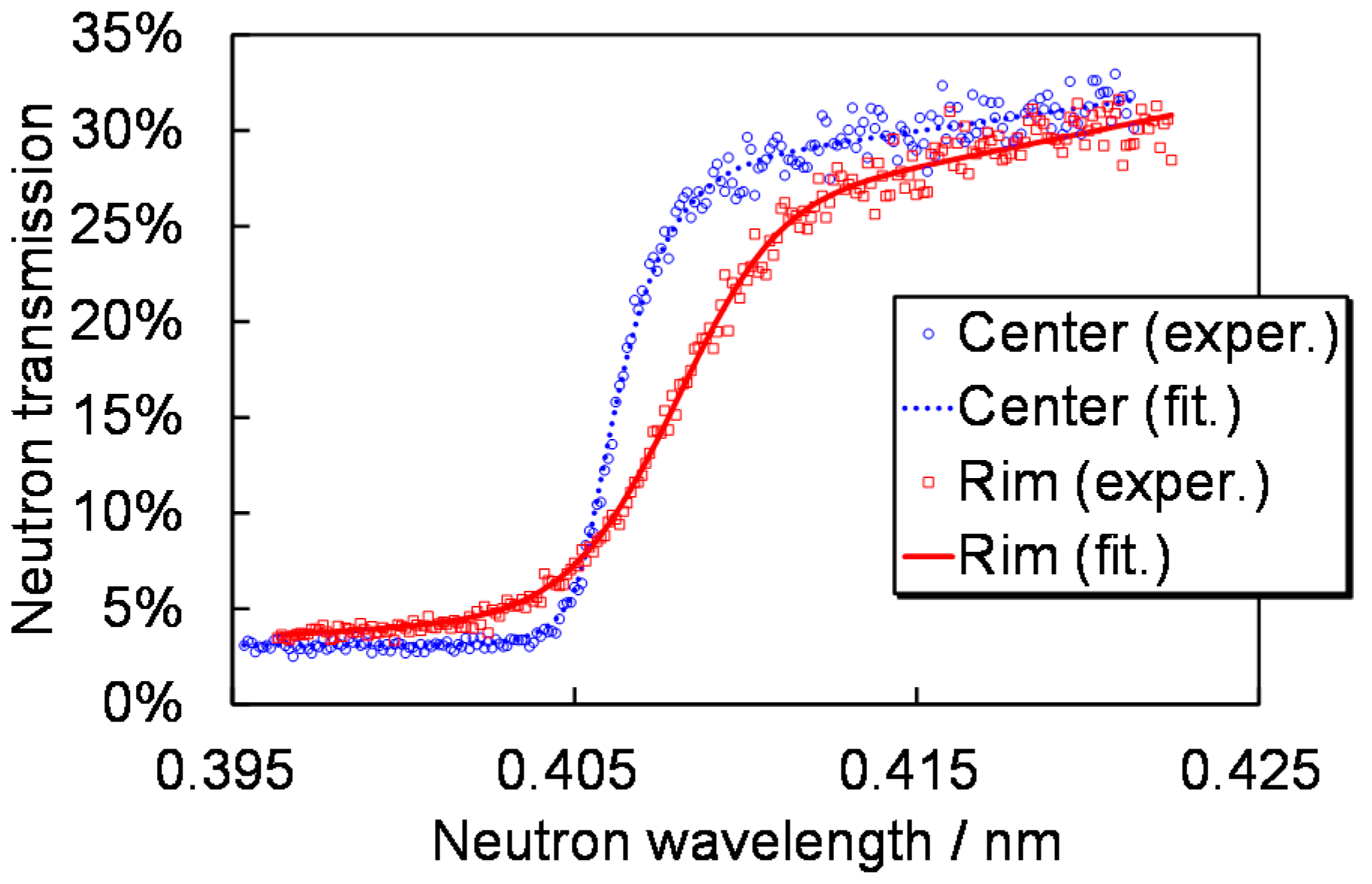
Figure 12 shows the measured transmission spectra near {110} Bragg-edge of the center (ferrite) zone and the rim (martensite) zone, with the fitting curves. This figure indicates martensite has micro-strain because Bragg-edge of the martensite was broadened. By using the ferrite data without micro-strain, parameters of the instrumental wavelength resolution function σ0,110, α110 and β110 (see Section 2.2.3) were determined. Then, d110 (crystal lattice plane spacing, relating to macro-strain) and w110 (broadening of d110’s distribution, relating to micro-strain) were evaluated and visualized.
5.3. Imaging Results
The analyses using the RITS code were performed at each pixel of the imaging detector. Figure 13 shows imaging results of d110 (crystal lattice plane spacing, relating to macro-strain) and w110 (broadening of d110’s distribution, relating to micro-strain) of each quenched depth rod. Note that two same-type rods were simultaneously measured. d110 and w110 become larger at the rim (martensite) zone due to dislocation-density’s increase and/or fine microstructures caused by solid solution of carbon atoms into the crystal lattice. In addition, the depth of large d110 and w110 zone from the outer rim surface seems to correspond to the aimed quenched depth (3 mm, 5 mm and 7 mm). Actually, according to the Vickers hardness measurements, positions of the boundary between high d110/w110 zone and low d110/w110 zone correspond to positions indicating Hv 450 (hardness boundary between martensite and ferrite) [6]. In other words, this type of imaging also indicates crystalline phase imaging of martensite in a ferritic steel.
Figure 14 shows comparison result of relation between the Vickers hardness and w110 at the same positions of each specimen. This result indicates the Vickers hardness is proportional to w110. Since the Vickers hardness is also proportional to ferrite/martensite ratio, imaging of w110 obtained by this method can quantitatively visualize distributions of the martensite phase and the hardness in a ferritic steel.
5.4. Current Status at Compact Accelerator Driven Pulsed Neutron Sources
At the Hokkaido University Neutron Source (HUNS), a high-wavelength-resolution type decoupled moderator and a supermirror guide tube were installed at the thermal neutron beam-line [47]. As a result, the wavelength resolution for cold neutrons achieved 0.5% at the 6 m position from the moderator and quantitative imaging experiments of dhkl and whkl by using Bragg-edge transmission imaging were successfully demonstrated [47]. The dhkl and whkl values visualized at HUNS corresponded to those visualized at J-PARC although the total measurement time required 73 hours [47].
In the coupled moderator (low wavelength resolution) case, changes of the crystal lattice plane spacing of carbon anode inside a Li-ion battery product were successfully visualized at HUNS [48].
5.5. Check by Neutron Diffraction
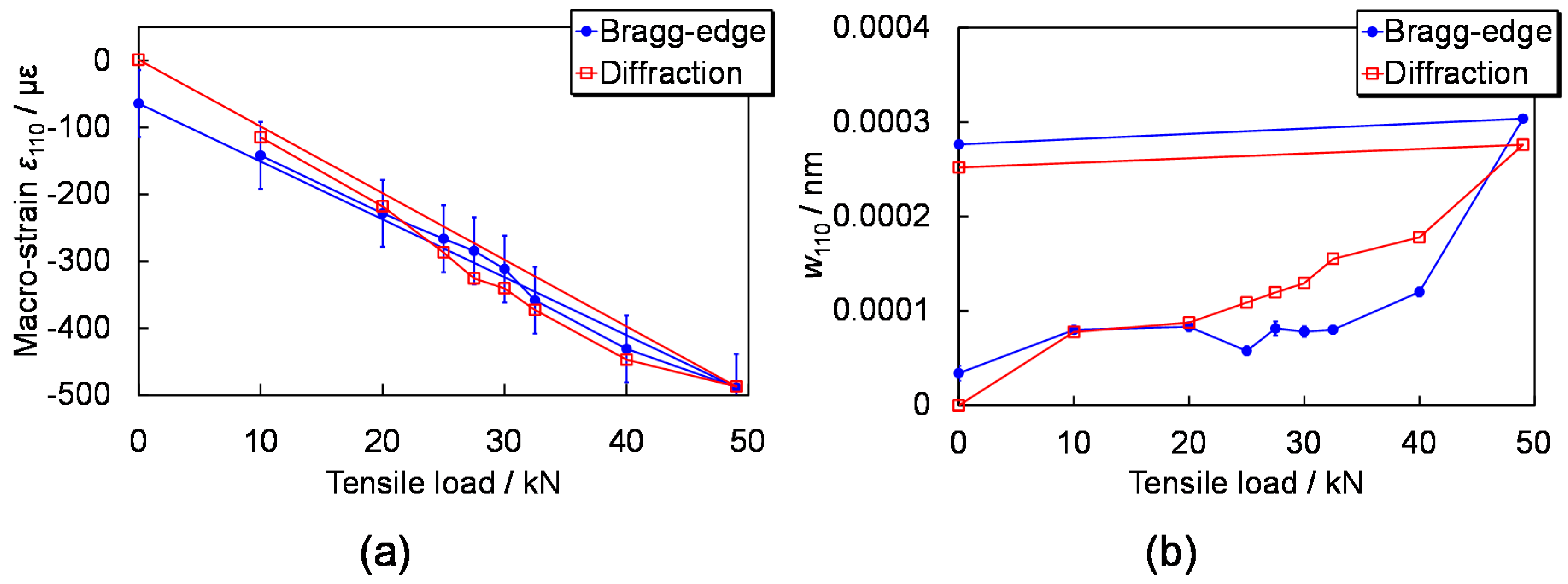
Figure 15a shows comparison results of macro-strain ε110 [3] and Figure 15b shows comparison results of w110 relating to micro-strain [8], between Bragg-edge transmission experiment and neutron diffraction experiment. The simultaneous experiment of transmission and diffraction was performed at J-PARC MLF BL19 “TAKUMI” [49]. The sample was an α-Fe plate of 5 mm thickness under tensile testing. In-situ measurements depending on the tensile load were carried out. Since the observed macro-strain direction is perpendicular to the tensile direction, negative macro-strain was observed. Incidentally, the Bragg-edge transmission data were measured by 6Li-glass scintillator pixel detector developed by Hokkaido University and KEK [50].
Figure 15a indicates that the difference between transmission result and diffraction result was about ±50 με. This value is close to the macro-strain resolution of the TAKUMI beam-line. Figure 15b also indicates the evaluated values are consistent between both methods. It is estimated that the differences between both methods are caused by difference of the gauge volume (diffraction-origin grains). In any case, it is confirmed that εhkl and whkl obtained by Bragg-edge transmission imaging are reliable. In particular, for the latter (micro-strain), this means that Bragg-edge broadening analysis method can be based on the same method used for neutron diffraction. Therefore, the dislocation density analysis [51] is expected for also Bragg-edge neutron transmission method in the future.
6. Development of Tensor CT Algorithm for Macro-Strain Tomography
Macro-strain is not scalar value but tensor value, which is different from quantity of crystalline phase (scalar value) etc. The algorithm of CT (computed tomography) is generally applicable to reconstruction of cross-sectional image of distribution of only scalar physical quantity such as density (absorption-contrast imaging) and refractive index (phase-contrast imaging); CT image reconstruction of tensor physical quantity such as macro-strain is impossible in principle. Although various approaches for macro-strain tomography are successfully in progress [52,53], an approach, development of the versatile (small restriction) tensor CT algorithm [54], is presented here. The details were reported in Reference [54].
6.1. Algorithm Based on the Maximum Likelihood - Expectation Maximization
First of all, the macro-strain at a certain position, εφψ observed along a direction φ and ψ tilted from a certain axes set, can be described by:
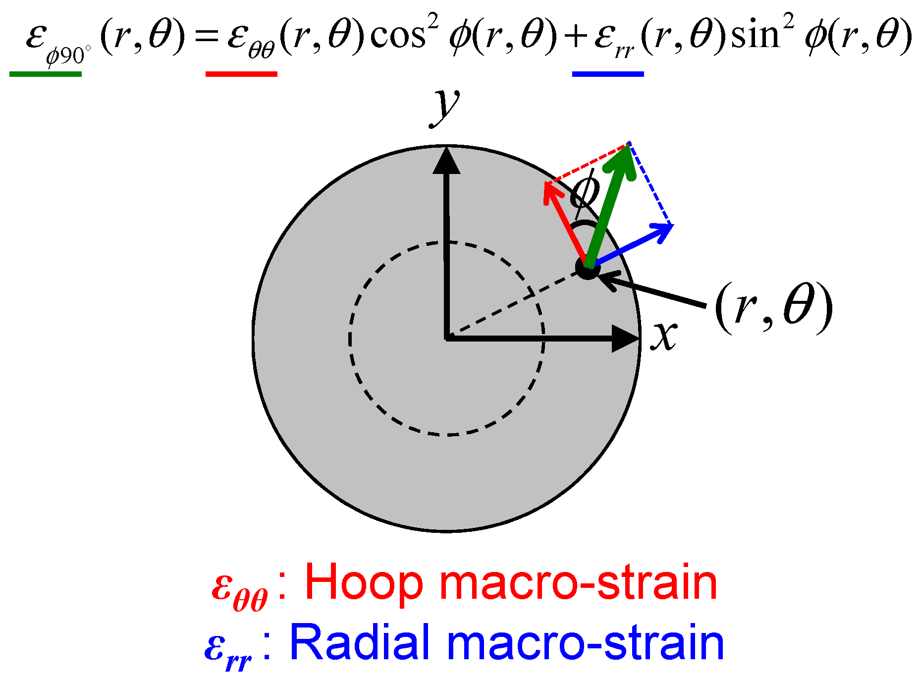
Here, ε11, ε22 and ε33 are normal strains along the axes 1, 2 and 3, respectively. ε12, ε23 and ε31 are shear strains from axis 1 to axis 2, from axis 2 to axis 3 and from axis 3 to axis 1, respectively. In this paper, the macro-strain “scalar” components means these parameters. These angle-unchangeable components have to be reconstructed individually from angle-changeable εφψ information (projection data). Since these six components are connected by the sine/cosine angle-dependent coefficients as a function of the angles φ and ψ, εφψ is angle-changeable. Incidentally, in case of axial-symmetric distribution, εφψ can be described by using the circular coordinates (r,θ) for the position in the tomographic cross-section:
Here, εθθ is macro-strain scalar component along the hoop direction and εrr is macro-strain scalar component along the radial direction.
For solving the tomographic reconstruction problem, an iterative-approximation approach using the maximum likelihood-expectation maximization (ML-EM) [55] was proposed [54]. The equation of the iteration from the trial k to the trial k+1 is:
ε is a certain macro-strain scalar component. i indicates a position in a cross-sectional plane of CT image (the total amount is I), j means jth scalar component (the total amount is J) and d indicates a detector pixel (the total amount is D). Cid is a geometrical detection probability of the position i by the detector d. Aijd is the most important parameter for the tensor CT algorithm, a detection probability of jth component of the position i by the detector d. Aijd has a function to express the angular dependence of the observed quantity; in other words, this parameter corresponds to the angle-dependent (sine/cosine) coefficients in Equations (27) and (28). n indicates the weight of Aijd for the back-projection procedure in the ML-EM procedure. pd is the so-called projection data that is the line-integrated value of a physical quantity (crystal lattice plane spacing, in this study) for the neutron transmission path covered by the detector d. Equation (29) is almost same as the general scalar CT algorithm using ML-EM, except for Aijd. This means this method is a versatile method, based on simple algorithm with small limitations. By using this quite simple method, macro-strain tomography was demonstrated [54].
6.2. Experimental
The measured sample was the VAMAS (Versailles Project on Advanced Materials and Standards) sample which is the aluminum shrink-fit ring and plug and is an international standard sample for neutron diffraction strain analysis [56]. Figure 16 shows a schematic layout of cross-sectional distribution in the VAMAS sample. The size of the VAMAS sample is 5 cm in diameter and 5 cm in height. The macro-strain distribution is axial symmetric which can be described by Equation (28). For this sample, projection data of d-spacing of Al {111} were measured by a Bragg-edge transmission imaging experiment and then macro-strain tomographic images of εθθ and εrr were reconstructed by the ML-EM based tensor CT method and Equation (2). Incidentally, the neutron beam was transmitted along the x direction (see Figure 16) since this is a tomography experiment.
The experiment was performed at J-PARC MLF BL10 “NOBORU” [33]. The power of the 3 GeV proton synchrotron of J-PARC was 300 kW during the experiment. The cold-neutron flux at the detector position was about 0.8×10⁶ n/cm2/s. The cold-neutron wavelength resolution was about 0.35%. The collimator ratio L/D was 600 (the beam angular divergence was 1.6 mrad). The used neutron TOF-imaging detector was GEM [38] which has the pixel size of 800 μm and the detection area of 10.24 cm × 10.24 cm. The measurement time for sample beam was 16 hours and the measurement time for open beam was 16 hours. Only one direction measurement was performed because the sample was axial symmetric.
6.3. Tomographic Imaging Results
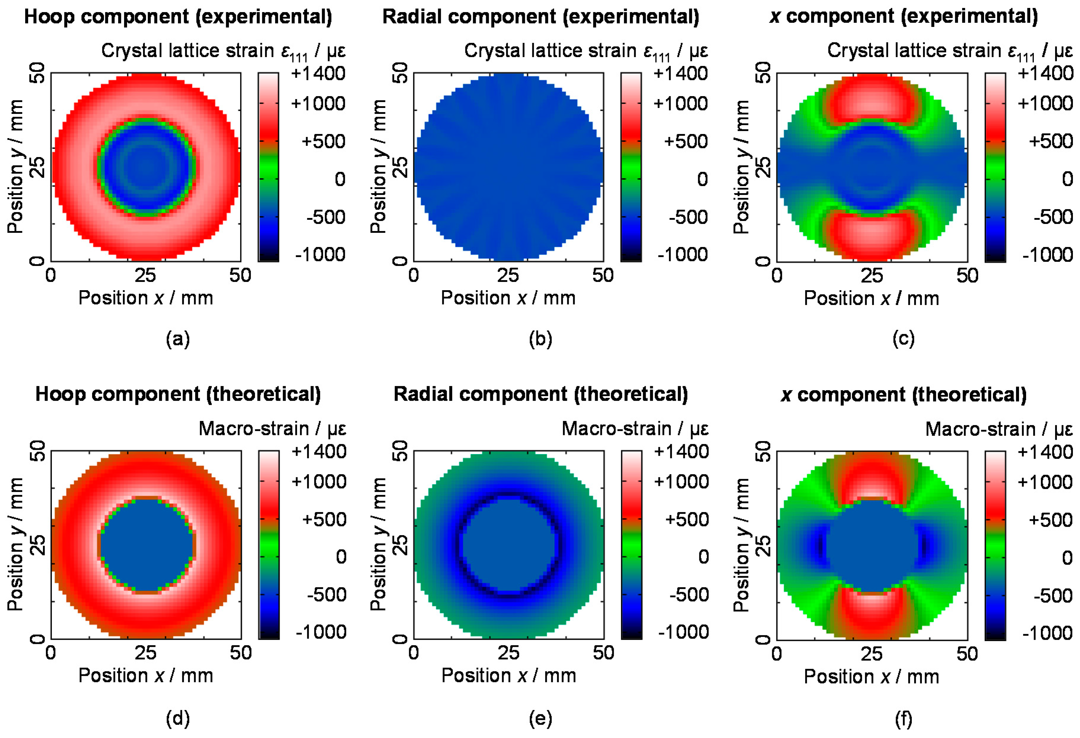
The evaluated projection data (raw and smoothed) are shown in Figure 17 with the theoretical values. Figure 18 shows the tomographic imaging results of (a) hoop macro-strain component εθθ, (b) radial macro-strain component εrr and (c) x-direction macro-strain component made from (a) and (b), respectively. The theoretical values of (d) hoop macro-strain, (e) radial macro-strain and (f) x-direction macro-strain made from (d) and (e) are also shown in Figure 18.
The number of iteration of the ML-EM based tensor CT procedure was 30 times and the number of projection was 16 directions. The same 16-angles projection data (Figure 17) were assumed owing to the axial symmetric distribution. The angle-dependent coefficients Aijd in Equation (29) were assumed as sine/cosine coefficients of Equation (28). The weight n of Equation (29) was set in 16. Macro-strain values were calculated by using Equation (2) after the reconstruction of tomographic image of crystal lattice plane spacing d111 of Al {111}.
According to Figure 18, hoop macro-strain tomography was successfully reconstructed but radial macro-strain tomography was not successful. Since the tensor CT is difficult non-linear problem in principle, some restrictions for the improvement are necessary for more accurate reconstruction. Incidentally, the developed versatile tensor CT algorithm is applicable for asymmetric macro-strain tomography [54]. However, it has been reported that a perfect CT image reconstruction without any restrictions is not easy as well as the presented symmetric macro-strain tomography case.
7. Grain Orientation Imaging by Bragg-Dip Pattern Analysis
By using the Bragg-dip pattern analysis method presented in Section 2.3, grain orientation imaging using pulsed neutron transmission measurements was successfully demonstrated [28]. In this section, the results of grain orientation imaging over the bulk in a sample are presented.
7.1. Experimental
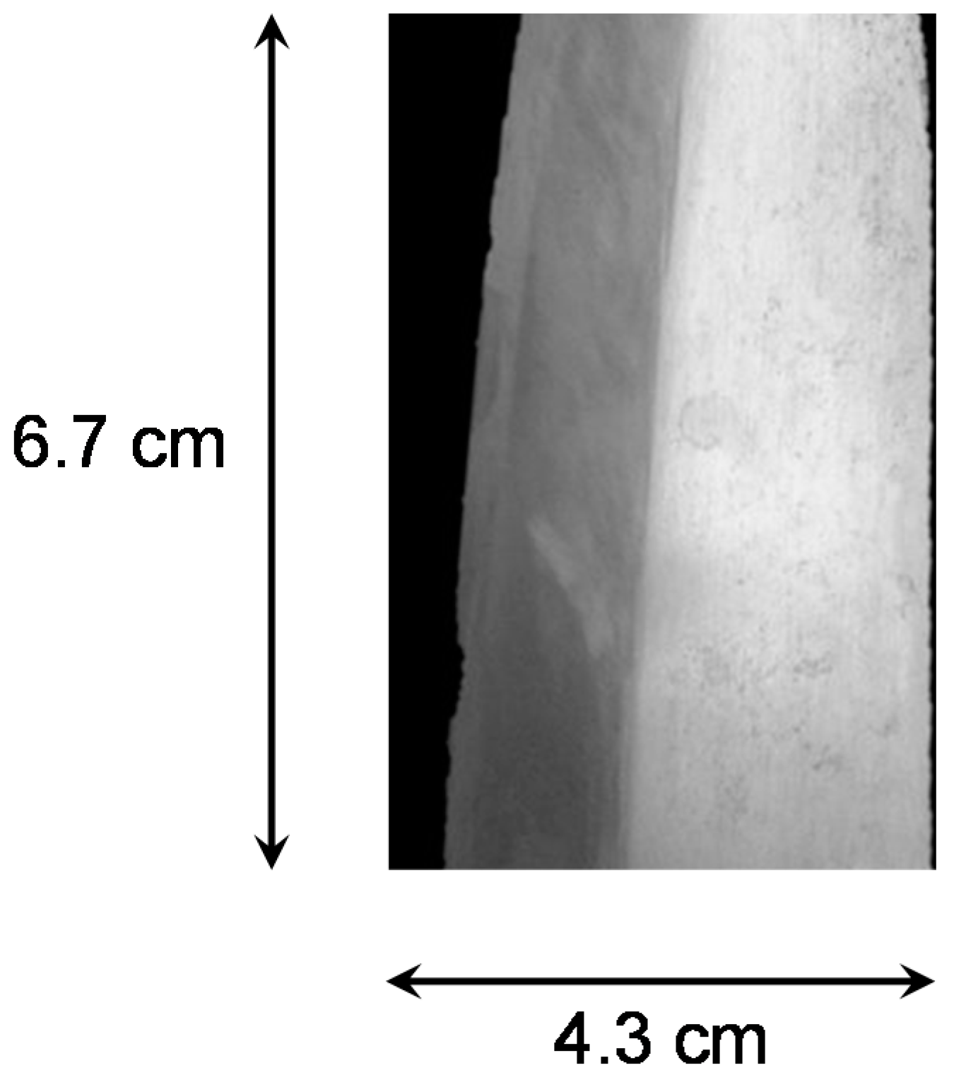
Figure 19 shows a photograph of the specimen. The sample was 3.4 wt % Si-steel plate (BCC crystal structure) of 5 mm thickness, which is generally used for an electromagnetic steel. This sample had large grains (see Figure 19). For this sample, the developed Bragg-dip pattern analysis (the database matching method) was applied and the number of grains and their crystal-lattice directions [UVW] along the neutron transmission direction were identified position-by-position.
The experiment was performed at J-PARC MLF BL10 “NOBORU” [33]. The power of the 3 GeV proton synchrotron of J-PARC was 500 kW during the experiment. The cold-neutron flux at the detector position was about 8 × 10⁴ n/cm2/s. The cold-neutron wavelength resolution was about 0.35%. The collimator ratio L/D was 2400 (the beam angular divergence was 0.4 mrad) because the size of B4C slit at the 7 m position was 3 mm × 3 mm. The used neutron TOF-imaging detector was the nGEM detector used in J-PARC MLF BL22 “RADEN” [57] which is the first pulsed neutron imaging instrument in the world. The detector had the pixel size of 800 μm and the detection area of 10.24 cm × 10.24 cm. The measurement time for sample beam was 14.5 hours and the measurement time for open beam was 7.2 hours.
7.2. Imaging Results
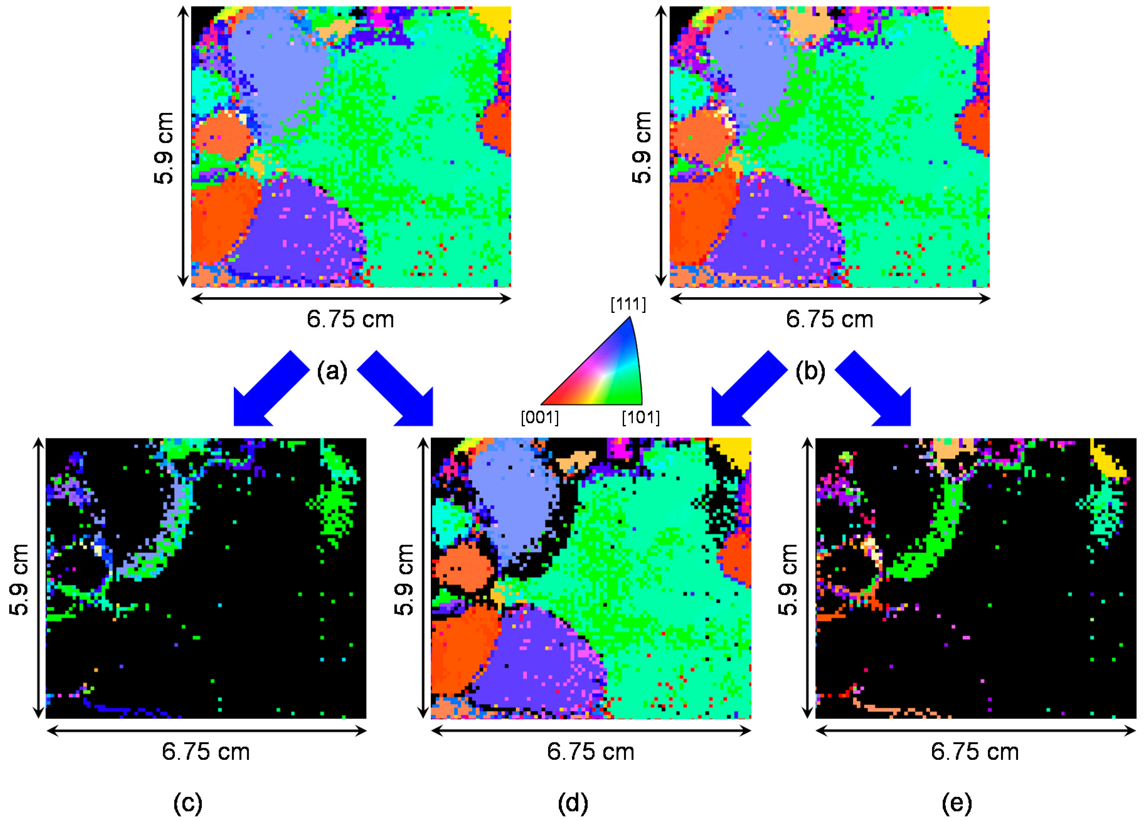
The Bragg-dip analyses using the database matching method were performed at each pixel of the imaging detector. Figure 20 shows results of IPF (inverse pole figure) imaging of the sample, obtained by Bragg-dip neutron transmission imaging experiment and the database matching method for Bragg-dip transmission spectrum. The crystal-lattice orientation expressed by IPF is parallel to the normal direction of the plate (the neutron transmission direction).
About Figure 20a,b, the same colour between the images means that only single grain exists along the neutron transmission path, as visualized by Figure 20d. The colour indicates crystal-lattice orientation parallel to the neutron transmission direction. On the other hand, the different colours between Figure 20a,b mean that two grains exist along the neutron transmission path, as visualized by Figure 20c,e. Each colour indicates crystal-lattice orientations of each grain, parallel to the neutron transmission direction. According to the database matching method, it was found that the maximum number of grains stacked along the neutron transmission path was only two in this sample. Thus, the Bragg-dip pattern analysis using the database matching method can quickly give the IPF images of all grains existing along the neutron transmission path. Incidentally, the reliability of the evaluated orientations is already discussed in Section 2.3.2.
8. Conclusions
This paper presents current status of quantitative imaging methods using Bragg-edge and Bragg-dip transmission analyses for bulk crystallographic information. For texture and crystallite size, the Rietveld-type analysis (the RITS code) is effective and the reliability was well confirmed by neutron diffraction Rietveld analysis. The Rietveld-type analysis is effective for accurate crystalline phase quantification because the RITS code has transmission-intensity correction functions for texture effect and crystallite-size effect. This reliability was also checked by neutron diffraction Rietveld analysis. Radiographic macro/micro-strain imaging is achieved by the single-edge profile analysis mode of RITS and the reliability was confirmed by neutron diffraction. The further development for dislocation density analysis is expected for Bragg-edge broadening analysis, as well as line-broadening analysis of diffraction peak. Although tomographic macro-strain imaging is quite difficult problem, it is not impossible for new CT reconstruction algorithms such as the tensor CT algorithm. Grain orientation imaging using Bragg-dip neutron transmission method is feasible by the presented new fast determination method for the number of grains and their orientations.
Thus, research and development activities within last 10 years greatly advance the possibility of the Bragg-edge/dip neutron transmission imaging for materials science and engineering. The construction projects of wavelength-resolved neutron imaging instruments at intense pulsed spallation neutron sources, J-PARC MLF BL22 “RADEN” [57], RAL ISIS-TS2 “IMAT” [58] and ESS “ODIN” [59], are going. At such world-leading facilities, higher level experiments will be performed than the experiments presented in this paper. Additionally, activities at compact accelerator driven pulsed neutron sources such as HUNS [35,36,44,47] are recently enhanced by collaboration between academic society and industrial society. The Bragg-edge/dip neutron transmission imaging is expected to become a key technology for materials characterization performed at both types of neutron beam facility.
Acknowledgements
The author is thankful to Y. Kiyanagi (Nagoya Univ.), T. Kamiyama (Hokkaido Univ.), T. Shinohara (J-PARC), M. Furusaka (Hokkaido Univ.), Y. Shiota (Metal Technology Co. Ltd.), K. Oikawa (J-PARC), Y. H. Su (J-PARC), K. Watanabe (Nagoya Univ.), K. Iwase (Ibaraki Univ.), S. Uno (KEK), A. S. Tremsin (UC Berkeley), K. Mochiki (Tokyo City Univ.), R. Kiyanagi (J-PARC), T. Kai (J-PARC), K. Sato (Hokkaido Univ.) and M. Ohnuma (Hokkaido Univ.).
Conflicts of Interest
The author declares no conflict of interest.
References
- Sato, H.; Kamiyama, T.; Kiyanagi, Y. A Rietveld-type analysis code for pulsed neutron Bragg-edge transmission imaging and quantitative evaluation of texture and microstructure of a welded α-iron plate. Mater. Trans. 2011, 52, 1294–1302. [Google Scholar] [CrossRef]
- Sato, H.; Kamiyama, T.; Iwase, K.; Ishigaki, T.; Kiyanagi, Y. Pulsed neutron spectroscopic imaging for crystallographic texture and microstructure. Nucl. Instrum. Methods A 2011, 651, 216–220. [Google Scholar] [CrossRef]
- Iwase, K.; Sato, H.; Harjo, S.; Kamiyama, T.; Ito, T.; Takata, S.; Aizawa, K.; Kiyanagi, Y. In situ lattice strain mapping during tensile loading using the neutron transmission and diffraction methods. J. Appl. Crystallogr. 2012, 45, 113–118. [Google Scholar] [CrossRef]
- Kiyanagi, Y.; Sato, H.; Kamiyama, T.; Shinohara, T. A new imaging method using pulsed neutron sources for visualizing structural and dynamical information. J. Phys. Conf. Ser. 2012, 340. [Google Scholar] [CrossRef]
- Sato, H.; Shinohara, T.; Kiyanagi, R.; Aizawa, K.; Ooi, M.; Harada, M.; Oikawa, K.; Maekawa, F.; Iwase, K.; Kamiyama, T.; et al. Upgrade of Bragg edge analysis techniques of the RITS code for crystalline structural information imaging. Phys. Procedia 2013, 43, 186–195. [Google Scholar] [CrossRef]
- Sato, H.; Sato, T.; Shiota, Y.; Kamiyama, T.; Tremsin, A.S.; Ohnuma, M.; Kiyanagi, Y. Relation between Vickers hardness and Bragg-edge broadening in quenched steel rods observed by pulsed neutron transmission imaging. Mater. Trans. 2015, 56, 1147–1152. [Google Scholar] [CrossRef]
- Sato, H.; Watanabe, K.; Kiyokawa, K.; Kiyanagi, R.; Hara, K.Y.; Kamiyama, T.; Furusaka, M.; Shinohara, T.; Kiyanagi, Y. Further improvement of the RITS code for pulsed neutron Bragg-edge transmission imaging. Phys. Procedia 2017, 88, 322–330. [Google Scholar] [CrossRef]
- Kamiyama, T.; Iwase, K.; Sato, H.; Harjo, S.; Ito, T.; Takata, S.; Aizawa, K.; Kiyanagi, Y. Microstructural information mapping of a plastic-deformed α-iron plate during tensile tests using pulsed neutron transmission. Phys. Procedia 2017, 88, 50–57. [Google Scholar] [CrossRef]
- Su, Y.H.; Oikawa, K.; Shinohara, T.; Kai, T.; Hiroi, K.; Harjo, S.; Kawasaki, T.; Gong, W.; Zhang, S.Y.; Parker, J.D.; et al. Time-of-flight neutron transmission imaging of martensite transformation in bent plates of a Fe-25Ni-0.4C alloy. Phys. Procedia 2017, 88, 42–49. [Google Scholar] [CrossRef]
- Rietveld, H.M. A profile refinement method for nuclear and magnetic structures. J. Appl. Crystallogr. 1969, 2, 65–71. [Google Scholar] [CrossRef]
- Marquardt, D.W. An algorithm for least-squares estimation of nonlinear parameters. J. Soc. Indust. Appl. Math. 1963, 11, 431–441. [Google Scholar] [CrossRef]
- Oba, Y.; Morooka, S.; Ohishi, K.; Sato, N.; Inoue, R.; Adachi, N.; Suzuki, J.; Tsuchiyama, T.; Gilbert, E.P.; Sugiyama, M. Magnetic scattering in the simultaneous measurement of small-angle neutron scattering and Bragg edge transmission from steel. J. Appl. Crystallogr. 2016, 49, 1659–1664. [Google Scholar] [CrossRef] [PubMed]
- Mamiya, H.; Oba, Y.; Terada, N.; Watanabe, N.; Hiroi, K.; Shinohara, T.; Oikawa, K. Magnetic Bragg dip and Bragg edge in neutron transmission spectra of typical spin superstructure. Sci. Rep. 2017, 7. [Google Scholar] [CrossRef] [PubMed]
- Petriw, S.; Dawidowski, J.; Santisteban, J. Porosity effects on the neutron total cross section of graphite. J. Nucl. Mater. 2010, 396, 181–188. [Google Scholar] [CrossRef]
- Oba, Y.; Morooka, S.; Ohishi, K.; Suzuki, J.; Takata, S.; Sato, N.; Inoue, R.; Tsuchiyama, T.; Gilbert, E.P.; Sugiyama, M. Energy-resolved small-angle neutron scattering from steel. J. Appl. Crystallogr. 2017, 50, 334–339. [Google Scholar] [CrossRef]
- Granada, J.R. Total scattering cross section of solids for cold and epithermal neutrons. Z. Naturforsch. A 1984, 39, 1160–1167. [Google Scholar] [CrossRef]
- Kropff, F.; Granada, J.R. CRIPO: A fast Computer Code for the Evaluation of σT in Polycrystalline Materials; Unpublished Report (CAB-1977); Centro Atomico Bariloche, Institute Balseiro: Bariloche, Argentina, 1977.
- Vogel, S. A Rietveld-Approach for the Analysis of Neutron Time-of-Flight Transmission Data. Ph.D. Thesis, Christian Albrechts Universität, Kiel, Germany, May 2000. [Google Scholar]
- Boin, M. NXS: A program library for neutron cross section calculations. J. Appl. Crystallogr. 2012, 45, 603–607. [Google Scholar] [CrossRef]
- Fermi, E.; Sturm, W.J.; Sachs, R.G. The transmission of slow neutrons through microcrystalline materials. Phys. Rev. 1947, 71, 589–594. [Google Scholar] [CrossRef]
- Von Dreele, R.B.; Jorgensen, J.D.; Windsor, C.G. Rietveld refinement with spallation neutron powder diffraction data. J. Appl. Crystallogr. 1982, 15, 581–589. [Google Scholar] [CrossRef]
- Larson, A.C.; Von Dreele, R.B. General Structure Analysis System (GSAS); Los Alamos National Laboratory Report LAUR 86-748; Los Alamos National Laboratory: Los Alamos, NM, USA, 2004.
- Dollase, W.A. Correction of intensities for preferred orientation in powder diffractometry: Application of the March model. J. Appl. Crystallogr. 1986, 19, 267–272. [Google Scholar] [CrossRef]
- Sabine, T.M. A reconciliation of extinction theories. Acta Crystallogr. Sec. A 1988, 44, 368–373. [Google Scholar] [CrossRef]
- Sabine, T.M.; Von Dreele, R.B.; Jørgensen, J.E. Extinction in time-of-flight neutron powder diffractometry. Acta Crystallogr. Sec. A 1988, 44, 374–379. [Google Scholar] [CrossRef]
- Santisteban, J.R.; Edwards, L.; Steuwer, A.; Withers, P.J. Time-of-flight neutron transmission diffraction. J. Appl. Crystallogr. 2001, 34, 289–297. [Google Scholar] [CrossRef]
- Santisteban, J.R.; Edwards, L.; Fitzpatrick, M.E.; Steuwer, A.; Withers, P.J.; Daymond, M.R.; Johnson, M.W.; Rhodes, N.; Schooneveld, E.M. Strain imaging by Bragg edge neutron transmission. Nucl. Instrum. Methods A 2002, 481, 765–768. [Google Scholar] [CrossRef]
- Sato, H.; Shiota, Y.; Morooka, S.; Todaka, Y.; Adachi, N.; Sadamatsu, S.; Oikawa, K.; Harada, M.; Zhang, S.Y.; Su, Y.H.; et al. Inverse pole figure mapping of bulk crystalline grains in a polycrystalline steel plate by pulsed neutron Bragg-dip transmission imaging. J. Appl. Crystallogr. 2017, 50, 1601–1610. [Google Scholar] [CrossRef]
- Santisteban, J.R. Time-of-flight neutron transmission of mosaic crystals. J. Appl. Crystallogr. 2005, 38, 934–944. [Google Scholar] [CrossRef]
- Malamud, F.; Santisteban, J.R. Full-pattern analysis of time-of-flight neutron transmission of mosaic crystals. J. Appl. Crystallogr. 2016, 49, 348–365. [Google Scholar] [CrossRef]
- Peetermans, S.; King, A.; Ludwig, W.; Reischig, P.; Lehmann, E.H. Cold neutron diffraction contrast tomography of polycrystalline material. Analyst 2014, 139, 5765–5771. [Google Scholar] [CrossRef] [PubMed]
- Cereser, A.; Strobl, M.; Hall, S.A.; Steuwer, A.; Kiyanagi, R.; Tremsin, A.S.; Knudsen, E.B.; Shinohara, T.; Willendrup, P.K.; Fanta, A.B.S.; et al. Time-of-flight three dimensional neutron diffraction in transmission mode for mapping crystal grain structures. Sci. Rep. 2017, 7. [Google Scholar] [CrossRef] [PubMed]
- Oikawa, K.; Maekawa, F.; Harada, M.; Kai, T.; Meigo, S.; Kasugai, Y.; Ooi, M.; Sakai, K.; Teshigawara, M.; Hasegawa, S.; et al. Design and application of NOBORU—NeutrOn Beam line for Observation and Research Use at J-PARC. Nucl. Instrum. Methods A 2008, 589, 310–317. [Google Scholar] [CrossRef]
- Seidel, L.; Hölscher, M.; Lücke, K. Rolling and recrystallization textures in iron-3% silicon. Textures Microstr. 1989, 11, 171–185. [Google Scholar] [CrossRef]
- Furusaka, M.; Sato, H.; Kamiyama, T.; Ohnuma, M.; Kiyanagi, Y. Activity of Hokkaido University Neutron Source, HUNS. Phys. Procedia 2014, 60, 167–174. [Google Scholar] [CrossRef]
- Sato, H.; Shiota, Y.; Kamiyama, T.; Ohnuma, M.; Furusaka, M.; Kiyanagi, Y. Performance of the Bragg-edge transmission imaging at a compact accelerator-driven pulsed neutron source. Phys. Procedia 2014, 60, 254–263. [Google Scholar] [CrossRef]
- Anderson, I.S.; Andreani, C.; Carpenter, J.M.; Festa, G.; Gorini, G.; Loong, C.-K.; Senesi, R. Research opportunities with compact accelerator-driven neutron sources. Phys. Rep. 2016, 654, 1–58. [Google Scholar] [CrossRef]
- Uno, S.; Uchida, T.; Sekimoto, M.; Murakami, T.; Miyama, K.; Shoji, M.; Nakano, E.; Koike, T.; Morita, K.; Sato, H.; et al. Two-dimensional neutron detector with GEM and its applications. Phys. Procedia 2012, 26, 142–152. [Google Scholar] [CrossRef]
- Ishigaki, T.; Hoshikawa, A.; Yonemura, M.; Morishima, T.; Kamiyama, T.; Oishi, R.; Aizawa, K.; Sakuma, T.; Tomota, Y.; Arai, M.; et al. IBARAKI materials design diffractometer (iMATERIA)—Versatile neutron diffractometer at J-PARC. Nucl. Instrum. Methods A 2009, 600, 189–191. [Google Scholar] [CrossRef]
- Oishi, R.; Yonemura, M.; Nishimaki, Y.; Torii, S.; Hoshikawa, A.; Ishigaki, T.; Morishima, T.; Mori, K.; Kamiyama, T. Rietveld analysis software for J-PARC. Nucl. Instrum. Methods A 2009, 600, 94–96. [Google Scholar] [CrossRef]
- Sato, H.; Sato, M.; Ishikawa, H.; Su, Y.H.; Shinohara, T.; Kamiyama, T.; Furusaka, M. Accuracy of quantification of crystalline phases evaluated by pulsed neutron Bragg-edge transmission imaging performed at J-PARC and HUNS. ISIJ Int. in preparation.
- Steuwer, A.; Withers, P.J.; Santisteban, J.R.; Edwards, L. Using pulsed neutron transmission for crystalline phase imaging and analysis. J. Appl. Phys. 2005, 97. [Google Scholar] [CrossRef]
- Woracek, R.; Penumadu, D.; Kardjilov, N.; Hilger, A.; Boin, M.; Banhart, J.; Manke, I. 3D mapping of crystallographic phase distribution using energy-selective neutron tomography. Adv. Mater. 2014, 26, 4069–4073. [Google Scholar] [CrossRef] [PubMed]
- Sato, H.; Mochiki, K.; Tanaka, K.; Ishizuka, K.; Ishikawa, H.; Kamiyama, T.; Kiyanagi, Y. A new high-speed camera type detector for time-of-flight neutron imaging and its application to crystalline phase analysis at a coupled-moderator based pulsed neutron source driven by a compact accelerator. Nucl. Instrum. Methods A. in preparation.
- Shiota, Y.; Hasemi, H.; Kiyanagi, Y. Crystallographic analysis of a Japanese sword by using Bragg edge transmission spectroscopy. Phys. Procedia 2017, 88, 128–133. [Google Scholar] [CrossRef]
- Tremsin, A.S.; McPhate, J.B.; Steuwer, A.; Kockelmann, W.; Paradowska, A.M.; Kelleher, J.F.; Vallerga, J.V.; Siegmund, O.H.W.; Feller, W.B. High-resolution strain mapping through time-of-flight neutron transmission diffraction with a microchannel plate neutron counting detector. Strain 2012, 48, 296–305. [Google Scholar] [CrossRef]
- Sato, H.; Sasaki, T.; Moriya, T.; Ishikawa, H.; Kamiyama, T.; Furusaka, M. High wavelength-resolution Bragg-edge/dip transmission imaging instrument with a supermirror guide-tube coupled to a decoupled thermal-neutron moderator at Hokkaido University Neutron Source. Physica B 2017. [Google Scholar] [CrossRef]
- Kamiyama, T.; Narita, Y.; Sato, H.; Ohnuma, M.; Kiyanagi, Y. Structural change of carbon anode in a lithium-ion battery product associated with charging process observed by neutron transmission Bragg-edge imaging. Phys. Procedia 2017, 88, 27–33. [Google Scholar] [CrossRef]
- Harjo, S.; Ito, T.; Aizawa, K.; Arima, H.; Abe, J.; Moriai, A.; Iwahashi, T.; Kamiyama, T. Current status of engineering materials diffractometer at J-PARC. Mater. Sci. Forum 2011, 681, 443–448. [Google Scholar] [CrossRef]
- Sato, H.; Takada, O.; Satoh, S.; Kamiyama, T.; Kiyanagi, Y. Development of material evaluation method by using a pulsed neutron transmission with pixel type detectors. Nucl. Instrum. Methods A 2010, 623, 597–599. [Google Scholar] [CrossRef]
- Ungár, T.; Harjo, S.; Kawasaki, T.; Tomota, Y.; Ribárik, G.; Shi, Z. Composite behavior of lath martensite steels induced by plastic strain, a new paradigm for the elastic-plastic response of martensitic steels. Metall. Mater. Trans. A 2017, 48, 159–167. [Google Scholar]
- Kirkwood, H.J.; Zhang, S.Y.; Tremsin, A.S.; Korsunsky, A.M.; Baimpas, N.; Abbey, B. Neutron strain tomography using the radon transform. Mater. Today Proc. 2015, 2, S414–S423. [Google Scholar] [CrossRef]
- Hendriks, J.N.; Gregg, A.W.T.; Wensrich, C.M.; Tremsin, A.S.; Shinohara, T.; Meylan, M.; Kisi, E.H.; Luzin, V.; Kirsten, O. Bragg-edge elastic strain tomography for in situ systems from energy-resolved neutron transmission imaging. Phys. Rev. Mater. 2017, 1. [Google Scholar] [CrossRef]
- Sato, H.; Shiota, Y.; Shinohara, T.; Kamiyama, T.; Ohnuma, M.; Furusaka, M.; Kiyanagi, Y. Development of the tensor CT algorithm for strain tomography using Bragg-edge neutron transmission. Phys. Procedia 2015, 69, 349–357. [Google Scholar] [CrossRef]
- Dempster, A.P.; Laird, N.M.; Rubin, D.B. Maximum likelihood from incomplete data via the EM algorithm. J. Royal Statistical Soc. Ser. B 1977, 39, 1–38. [Google Scholar]
- Webster, G.A. Neutron Diffraction Measurements of Residual Stress in A Shrink-Fit Ring and Plug; VAMAS Report 38; VAMAS TWA 20: London, UK, 2000; ISSN 1016-2186. [Google Scholar]
- Shinohara, T.; Kai, T.; Oikawa, K.; Segawa, M.; Harada, M.; Nakatani, T.; Ooi, M.; Aizawa, K.; Sato, H.; Kamiyama, T.; et al. Final design of the Energy-Resolved Neutron Imaging System “RADEN” at J-PARC. J. Phys. Conf. Ser. 2016, 746. [Google Scholar] [CrossRef]
- Kockelmann, W.; Burca, G.; Kelleher, J.F.; Kabra, S.; Zhang, S.Y.; Rhodes, N.J.; Schooneveld, E.M.; Sykora, J.; Pooley, D.E.; Nightingale, J.B.; et al. Status of the neutron imaging and diffraction instrument IMAT. Phys. Procedia 2015, 69, 71–78. [Google Scholar] [CrossRef]
- Strobl, M. The scope of the imaging instrument project ODIN at ESS. Phys. Procedia 2015, 69, 18–26. [Google Scholar] [CrossRef]
Figure 1.
(a) Bragg-edge transmission spectrum and the included crystallographic information. The specimen is a polycrystalline α-Fe of 5 mm thickness. (b) Bragg-dip transmission spectrum and the included crystallographic information. The specimen is a single-crystal α-Fe of 5 mm thickness. (Note that all the data were measured at J-PARC MLF.) Such transmission spectra are measured at each pixel of a neutron TOF-imaging detector. Therefore, through the transmission spectrum analyses at each pixel, various crystallographic information can be quantitatively mapped over the whole body of a measured specimen.
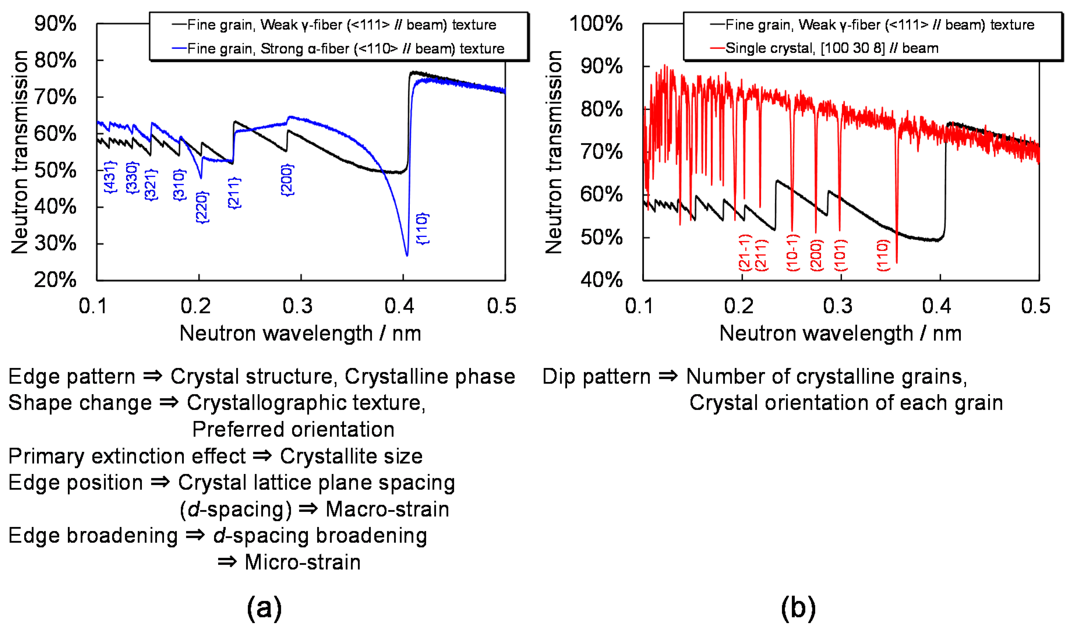
Figure 2.
Scheme of the database matching method. (Note that exampled neutron transmission spectra were measured by the experiment presented in Reference [28].) Even if a few grains are stacked along the neutron transmission path, the unique crystal-lattice direction [UVW] of each grain, parallel to the neutron transmission direction, are simultaneously identified by this method. This figure schematically indicates that [UVW] of one of stacked grains (Grain 1) is [100 70 53] and [UVW] of the other of stacked grains (Grain 2) is [100 75 27].

Figure 3.
Bragg-dip transmission spectra of (a) Grain Orientation 1 and (b) Grain Orientation 2 with the pattern matching results (cross × marks) and the indexing results. It is identified by the database matching method that [UVW] of Grain Orientation 1 is [100 30 8] and [UVW] of Grain Orientation 2 is [100 38 0]. These figures are reproduced with permission of the International Union of Crystallography from Reference [28].
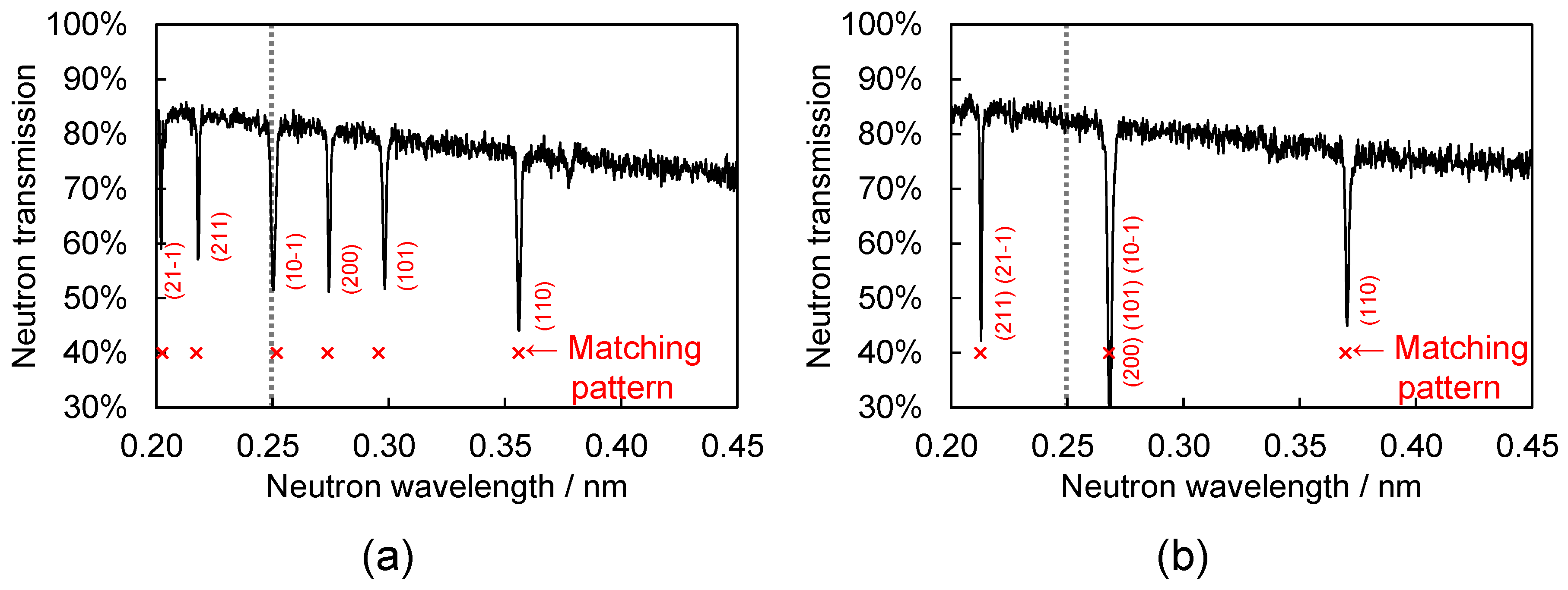
Figure 4.
Photograph of rolled/welded α-iron specimens for demonstration of quantitative texture and crystallite-size imaging [1]. Weld exists at the center of welded plates (Sample C and Sample D).
Figure 4.
Photograph of rolled/welded α-iron specimens for demonstration of quantitative texture and crystallite-size imaging [1]. Weld exists at the center of welded plates (Sample C and Sample D).
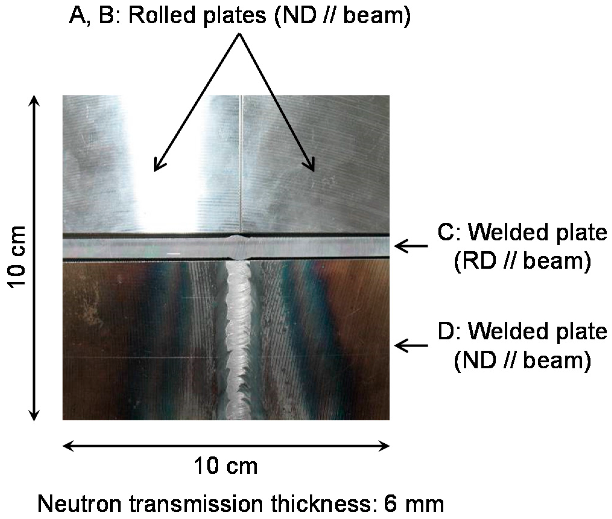
Figure 5.
Three types of Bragg-edge transmission spectrum with the fitting curves [1]. Due to the texture effect and the extinction effect, spectrum shape and spectrum intensity are changed. From these profile changes, degree of crystallographic anisotropy, preferred orientation and crystallite size are quantitatively deduced.
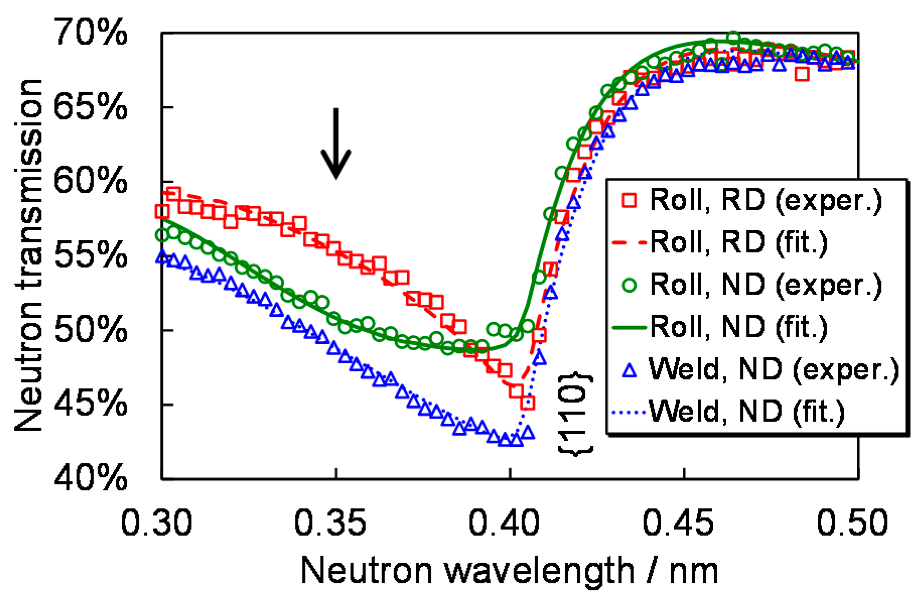
Figure 6.
Quantitative imaging results of (a) preferred orientation parallel to neutron transmission direction, (b) degree of texture evolution and (c) crystallite size averaged along neutron transmission direction [1,7].

Figure 7.
Comparison between Bragg-edge neutron transmission method with the RITS code and neutron diffraction method with the Rietveld analysis: (a) March-Dollase coefficient (degree of texture evolution) and (b) crystallite size [2,7,36].
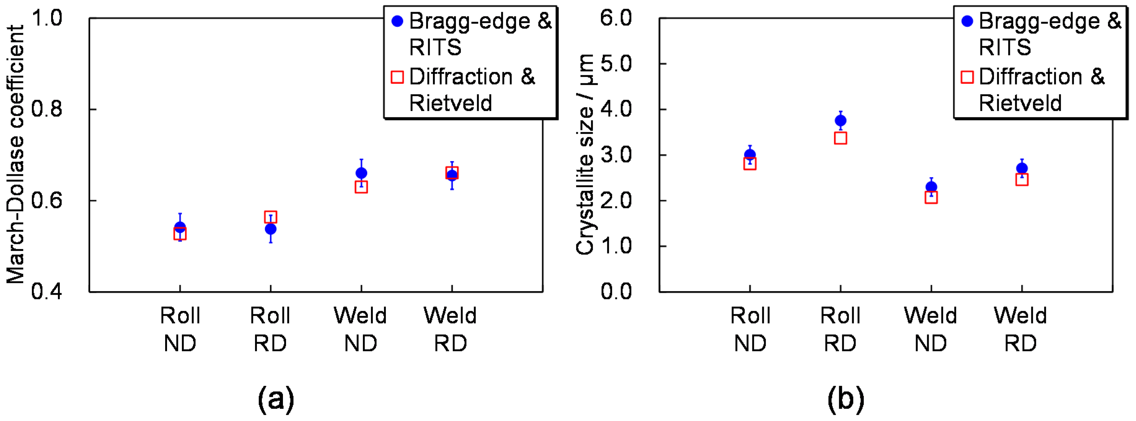
Figure 8.
Photograph of the knife specimen composed of α-Fe and γ-Fe [44]. The left-hand side is the cutting edge.
Figure 8.
Photograph of the knife specimen composed of α-Fe and γ-Fe [44]. The left-hand side is the cutting edge.

Figure 9.
Bragg-edge transmission spectrum of the knife specimen and the RITS fitting curves assuming single-phase and double-phase [44]. The double phase assumption is suitable for reconstruction of the experimental data. This means this specimen consists of double phase (α-Fe and γ-Fe).
Figure 9.
Bragg-edge transmission spectrum of the knife specimen and the RITS fitting curves assuming single-phase and double-phase [44]. The double phase assumption is suitable for reconstruction of the experimental data. This means this specimen consists of double phase (α-Fe and γ-Fe).

Figure 10.
Quantitative imaging of (a) α-Fe phase and (b) γ-Fe phase and the relating images: texture evolution of (c) α-Fe and (d) γ-Fe and crystallite size of (e) α-Fe and (f) γ-Fe [44].
Figure 10.
Quantitative imaging of (a) α-Fe phase and (b) γ-Fe phase and the relating images: texture evolution of (c) α-Fe and (d) γ-Fe and crystallite size of (e) α-Fe and (f) γ-Fe [44].

Figure 11.
Photograph of three types of quenched rod [6].
Figure 11.
Photograph of three types of quenched rod [6].

Figure 12.
{110} Bragg-edge of the unquenched center (ferrite) zone and the quenched rim (martensite) zone, with the profile fitting curves given by the single-edge analysis mode of RITS [6].
Figure 12.
{110} Bragg-edge of the unquenched center (ferrite) zone and the quenched rim (martensite) zone, with the profile fitting curves given by the single-edge analysis mode of RITS [6].

Figure 13.
(a–c) Images of crystal lattice plane spacing (d-spacing) of {110} [6]. (d–f) Images of FWHM of d-spacing distribution of {110} [6]. The pictures are visualized about each quenched depth (3 mm, 5 mm and 7 mm). Note that two rods of the same quenched depth are simultaneously visualized.
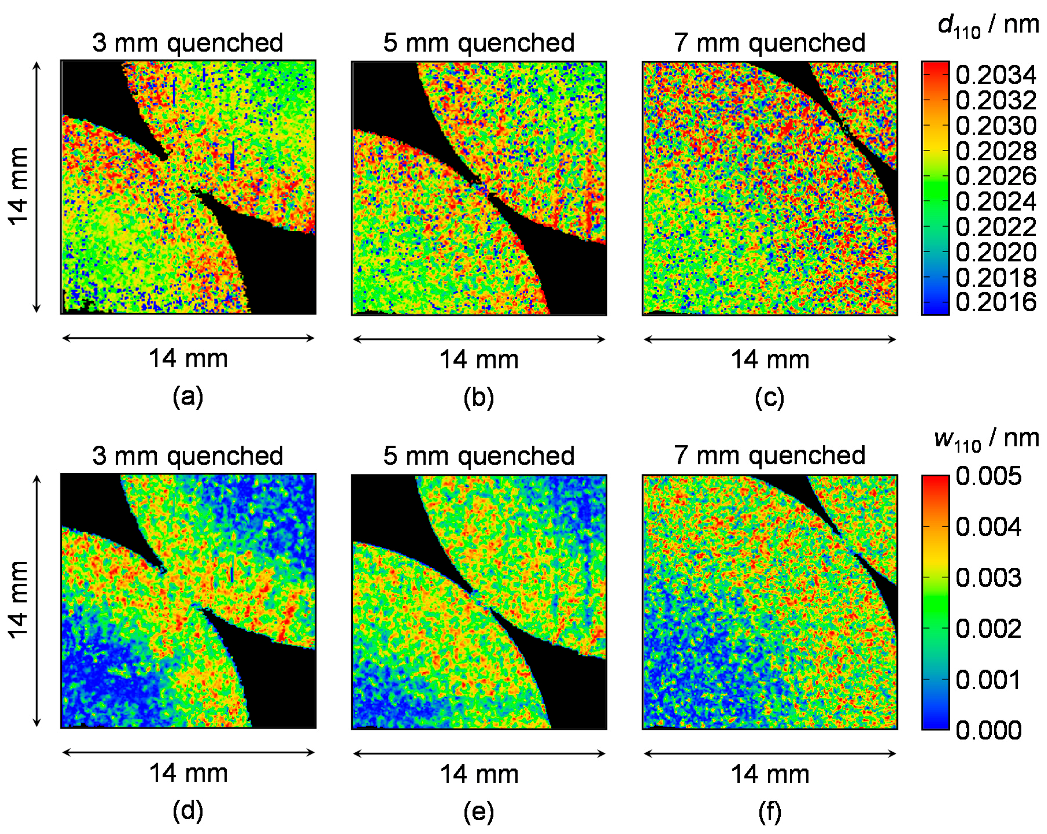
Figure 14.
Relation between the Vickers hardness and FWHM of d-spacing distribution, discovered by Bragg-edge neutron transmission imaging [6].
Figure 14.
Relation between the Vickers hardness and FWHM of d-spacing distribution, discovered by Bragg-edge neutron transmission imaging [6].
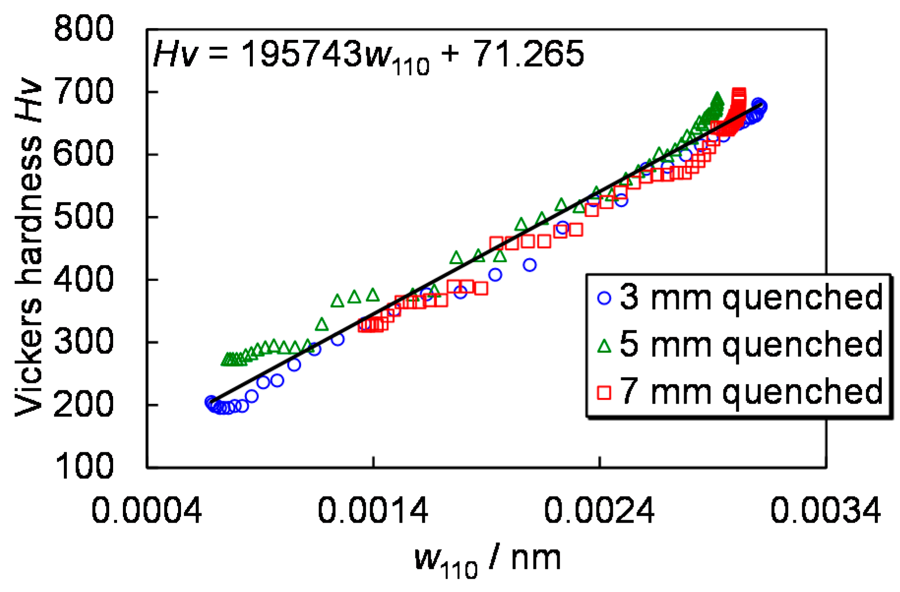
Figure 15.
Comparison between Bragg-edge neutron transmission and neutron diffraction: (a) macro-strain [3] and (b) FWHM of d-spacing distribution relating to micro-strain [8].

Figure 16.
Macro-strain scalar components (hoop component εθθ and radial component εrr) in the axial-symmetric VAMAS sample [54].
Figure 16.
Macro-strain scalar components (hoop component εθθ and radial component εrr) in the axial-symmetric VAMAS sample [54].

Figure 17.
Radial dependence of the projection data evaluated by RITS, its moving averaged (smoothed) data which were actually used for the CT image reconstruction and the theoretical values of projection data from the VAMAS cylinder [54].
Figure 17.
Radial dependence of the projection data evaluated by RITS, its moving averaged (smoothed) data which were actually used for the CT image reconstruction and the theoretical values of projection data from the VAMAS cylinder [54].
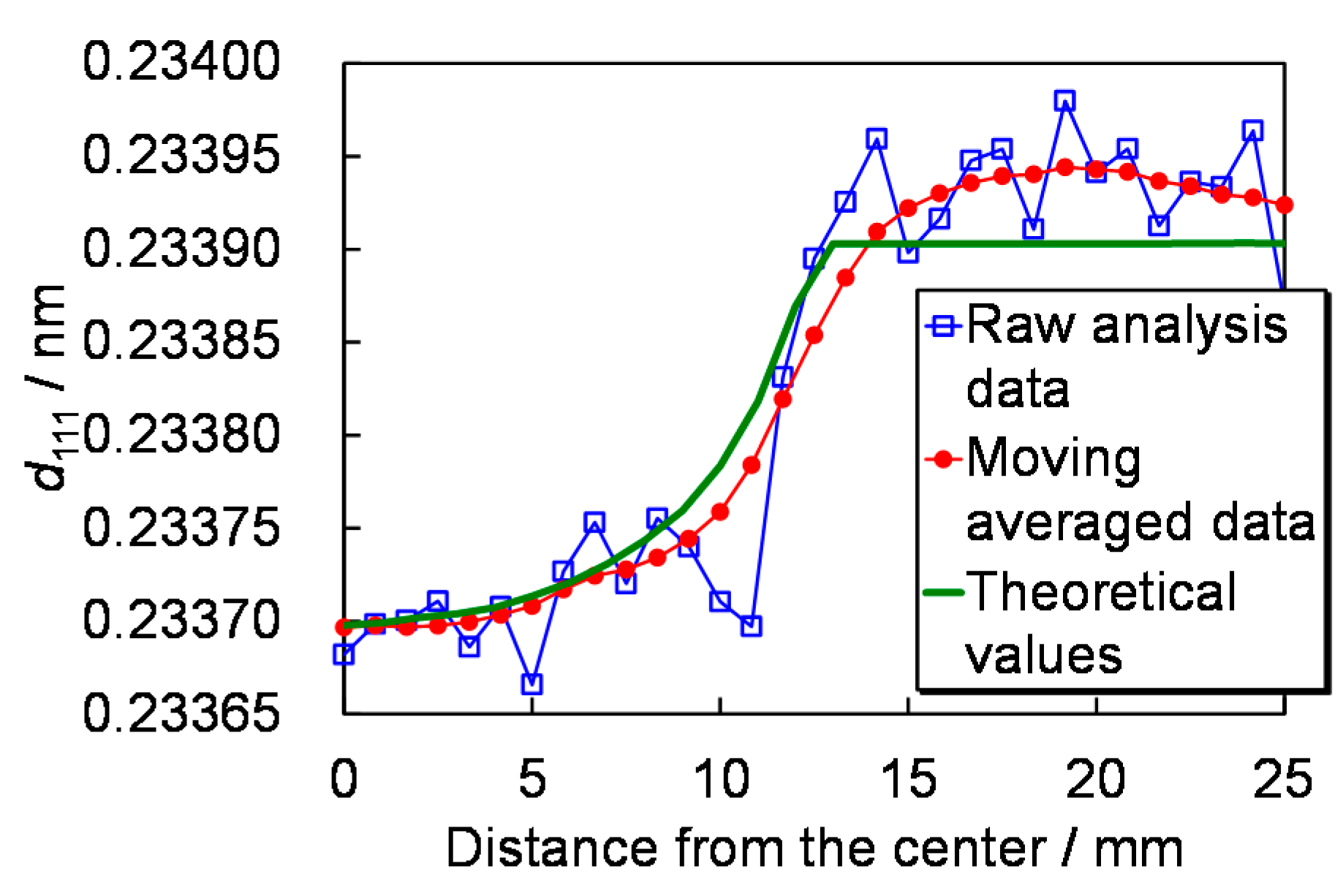
Figure 18.
Macro-strain tomography obtained by the ML-EM based tensor CT algorithm: (a) hoop component, (b) radial component and (c) x-direction component, with (d–f) their theoretical values [54].
Figure 18.
Macro-strain tomography obtained by the ML-EM based tensor CT algorithm: (a) hoop component, (b) radial component and (c) x-direction component, with (d–f) their theoretical values [54].

Figure 19.
Photograph of the Si-steel plate sample for demonstration of grain orientation imaging using Bragg-dip neutron transmission method [28].
Figure 19.
Photograph of the Si-steel plate sample for demonstration of grain orientation imaging using Bragg-dip neutron transmission method [28].
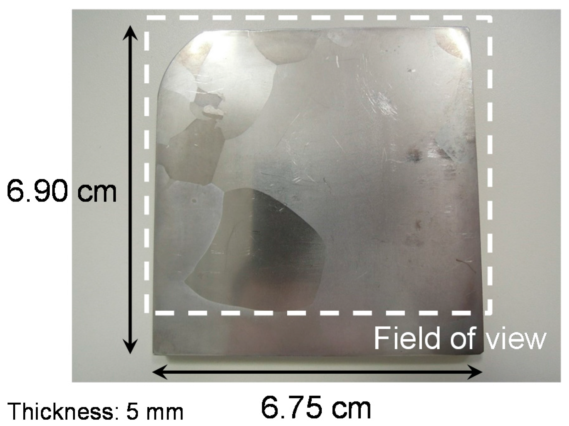
Figure 20.
Grain orientation images obtained by Bragg-dip neutron transmission analyses, expressed by inverse pole figure (IPF). (a) and (b) are images of all grains. (c)–(e) are partial images of the images (a) and (b). The image (d) indicates IPF map of a non-stacked grain along the neutron transmission path. The image (c) indicates IPF map of one of stacked grains along the neutron transmission path and the image (e) indicates IPF map of the other of stacked grains along the neutron transmission path. The image (a) is a combined image of the image (d) and the image (c) and the image (b) is a combined image of the image (d) and the image (e). These figures are reproduced with permission of the International Union of Crystallography from Reference [28].
© 2017 by the author. Licensee MDPI, Basel, Switzerland. This article is an open access article distributed under the terms and conditions of the Creative Commons Attribution (CC BY) license (http://creativecommons.org/licenses/by/4.0/).
Share and Cite
MDPI and ACS Style
Sato, H. Deriving Quantitative Crystallographic Information from the Wavelength-Resolved Neutron Transmission Analysis Performed in Imaging Mode. J. Imaging 2018, 4, 7. https://doi.org/10.3390/jimaging4010007
AMA Style
Sato H. Deriving Quantitative Crystallographic Information from the Wavelength-Resolved Neutron Transmission Analysis Performed in Imaging Mode. Journal of Imaging. 2018; 4(1):7. https://doi.org/10.3390/jimaging4010007
Chicago/Turabian StyleSato, Hirotaka. 2018. "Deriving Quantitative Crystallographic Information from the Wavelength-Resolved Neutron Transmission Analysis Performed in Imaging Mode" Journal of Imaging 4, no. 1: 7. https://doi.org/10.3390/jimaging4010007
Note that from the first issue of 2016, this journal uses article numbers instead of page numbers. See further details here.