Denoising of X-ray Images Using the Adaptive Algorithm Based on the LPA-RICI Algorithm


Faculty of Engineering, University of Rijeka, Vukovarska 58, 51000 Rijeka, Croatia
*
Author to whom correspondence should be addressed.
J. Imaging 2018, 4(2), 34; https://doi.org/10.3390/jimaging4020034
Submission received: 5 December 2017
/
Revised: 1 February 2018
/
Accepted: 2 February 2018
/
Published: 5 February 2018
Abstract
:Diagnostics and treatments of numerous diseases are highly dependent on the quality of captured medical images. However, noise (during both acquisition and transmission) is one of the main factors that reduce their quality. This paper proposes an adaptive image denoising algorithm applied to enhance X-ray images. The algorithm is based on the modification of the intersection of confidence intervals (ICI) rule, called relative intersection of confidence intervals (RICI) rule. For each image pixel apart, a 2D mask of adaptive size and shape is calculated and used in designing the 2D local polynomial approximation (LPA) filters for noise removal. One of the advantages of the proposed method is the fact that the estimation of the noise free pixel is performed independently for each image pixel and thus, the method is applicable for easy parallelization in order to improve its computational efficiency. The proposed method was compared to the Gaussian smoothing filters, total variation denoising and fixed size median filtering and was shown to outperform them both visually and in terms of the peak signal-to-noise ratio (PSNR) by up to 7.99 dB.
1. Introduction
Denoising (both of one-dimensional and multi-dimensional signals) is one of the most important fields in signal processing and hence, the pursuit for novel and more efficient denoising methods is constant [1]. Numerous methods developed over the last few decades found their applications in various fields, including medical image processing and analysis leading to enhancements in examining the interior of the human body without surgeries. However, since both revealing and treatment of large number of diseases today is highly dependent on medical images (such as computed tomography (CT), ultrasound, magnetic resonance imaging (MRI), X-rays etc.), improving their quality is an essential precondition for their analysis. One of the main problems with captured medical images is the presence of noise (introduced during both acquisition and transmission processes), which complicates their visual inspection and pathology pattern recognition. Thus, noise has to be suppressed in order to decrease the probability of possible misinterpretations and incorrect diagnoses [2].
Due to their cost and a decrease in the dose of ionizing radiation, X-rays are still the most frequently used medical imaging technique. However, lower doses of radiation require more efficient noise reduction methods such that the important image features (object contours, edges, textures, etc.) are preserved while the noise is smoothed.
There are numerous techniques for reducing noise from medical images, which can be classified into two main categories. First are the methods for image processing in the spatial domain and the second are the transform domain filtering approaches [3]. Spatial filtering methods may be divided into linear (such as, for example, mean and Wiener based filtering) and non-linear methods (for example, median and weighted median based filtering) [3]. However, the linear spatial domain filtering fails in case of signal dependent noise and, unfortunately, it also introduces blurring artefacts to denoised images [4,5]. On the other hand, transform domain image processing approaches may be divided into data adaptive methods (for example, independent component analysis) and non-data adaptive methods (such as wavelet domain and spatial-frequency domain processing algorithms) [3]. Unlike the spatial methods, the transform domain-based methods transform images from spatial into transform domain and noise is removed in the transform domain [4]. Next, the estimate of the noise-free image is obtained by applying the inverse transform.
The method proposed in the paper introduces an algorithm for medical image processing based on the adaptive, data-adaptive 2D spatial filters designed using the local polynomial approximation (LPA) combined with the modification of the intersection of confidence intervals (ICI) rule, called the relative intersection of confidence intervals (RICI) rule (where RICI rule determines the size of the LPA estimators).
The 2D LPA-RICI based algorithm has been shown to be an efficient noise-free image estimator, since the RICI based algorithm calculates the near optimal estimator size and its 2D shape for each considered pixel [6,7]. Unlike the approaches based on the fixed size filters, the given method (due to its couture and edge preserving property) smoothes the noise locally in the vicinity of the considered pixel and hence avoids blurring artefacts in the resulting denoised images.
Once calculated, adaptive 2D regions are used as binary masks for segmentation and extraction of the regions of interest from the original image. The noise-free estimate of the considered pixel is found by applying the LPA weighted averaging to the extracted region. The described procedure is repeated independently for each image pixel separately. Thus, one of the important advantages of the proposed 2D LPA-RICI based image denoising algorithm is that it may be easily parallelized in order to improve the method’s computational efficiency.
The proposed adaptive 2D LPA-RICI method was applied to denoising of real-life medical X-ray images, outperforming competitive methods (Gaussian smoothing filters, total variation denoising and fixed size median filtering) in most cases.
2. The ICI Rule and Its Modification
2.1. The ICI Algorithm
The LPA-ICI method utilizes the LPA for designing estimators, the size of which is data-driven and, hence, chosen adaptively using the ICI based rule. This section presents original one-dimensional ICI rule and its modification (the RICI rule) extended to denoising 2D medical images. A software for the original 1D ICI and 1D RICI signal denoising is made available by the author in [8].
Therefore, before we propose the 2D version of the RICI algorithm, let us introduce the original 1D signal filtering procedure.
Firstly, in order to obtain the estimate of the noise free signal, the ICI algorithm introduce a range of K estimators with increasing widths hi [6,7]:
and the corresponding confidence intervals , 1 ≤ ≤ K, defined for each signal sample n with interval limits (upper () and lower ()) defined as [6,7] (Katkovnik et al. 2005, 2002):
where defines the confidence level, represents the standard deviation of the estimation error and is calculated as the LPA weighted average of samples neighboring the considered -th sample [6,7].
H = {h1 < h2 < ⋯ < hK},
The procedure is repeated as long as all subsequent intervals are overlapping (or until the edges of the signal are reached). Namely, the ICI algorithm tracks the values of the smallest upper and the largest lower limits of the confidence interval defined as [6,7]:
as long as the lower interval limit is equal to or smaller than the upper interval limit (meaning that all subsequent intervals are overlapping) [6,7]:
Finally, the optimal filter width is determined as the largest for which all previous confidence intervals, including the -th interval, are overlapping [6,7].
As shown in [9], small hk values increase the estimate error variance and decrease its bias. On the other hand, large hk values decrease the estimate error variance and increase its bias (dependent on the unknown high-order signal derivatives) [9]. The adaptive ICI based algorithm calculates the maximal hk, value which ensures the optimal trade-off between the estimation bias and the variance. In other words, proper value results in the optimal smoothing effect since it ensures selecting the largest vicinity neighboring the considered point such that the LPA fits well to data [9]. Namely, small hk values are chosen for points close to rapid changes in the signal, while otherwise larger hk values are selected [9].
In order to justify previous claims, let us consider the absolute estimation error , calculated as:
where is a noise-free signal and its LPA estimate. The estimation error can be written as a sum of the bias and the zero-mean random error [9]:
Hence, the following inequity stands true [9]:
where is the maximal value of and is, in case of the Gaussian noise, zero-mean estimation error with the standard deviation . Furthermore, the following inequity holds true with the probability :
where is ()-th qantile of the normal distribution [9]. In other words, the estimation error is found inside the interval with the probability . From Equations (9) and (10) it follows that [9]:
holds true with the same probability [9]. It was shown that there exists an optimal , denoted as , providing an optimal estimation error bias to the variance trade-off, such that for [9]:
Thus, the inequity (12) can be written as:
or as:
where is lower and upper confidence interval limit, as given in Equations (2) and (3). Since both inequities (11) and (14) hold true with the probability , we can claim with the same probability that is inside the interval for [9]. In other words, a nonempty intersection of all subsequent confidence intervals ensures . On the other hand, an empty intersection of all subsequent confidence intervals means that [9]. Thus, the largest , as close as possible to , for which the intersection of all subsequent confidence intervals is nonempty, is to be chosen as the one giving the near optimal balance between the estimation error bias and the variance, as shown in Equation (6).
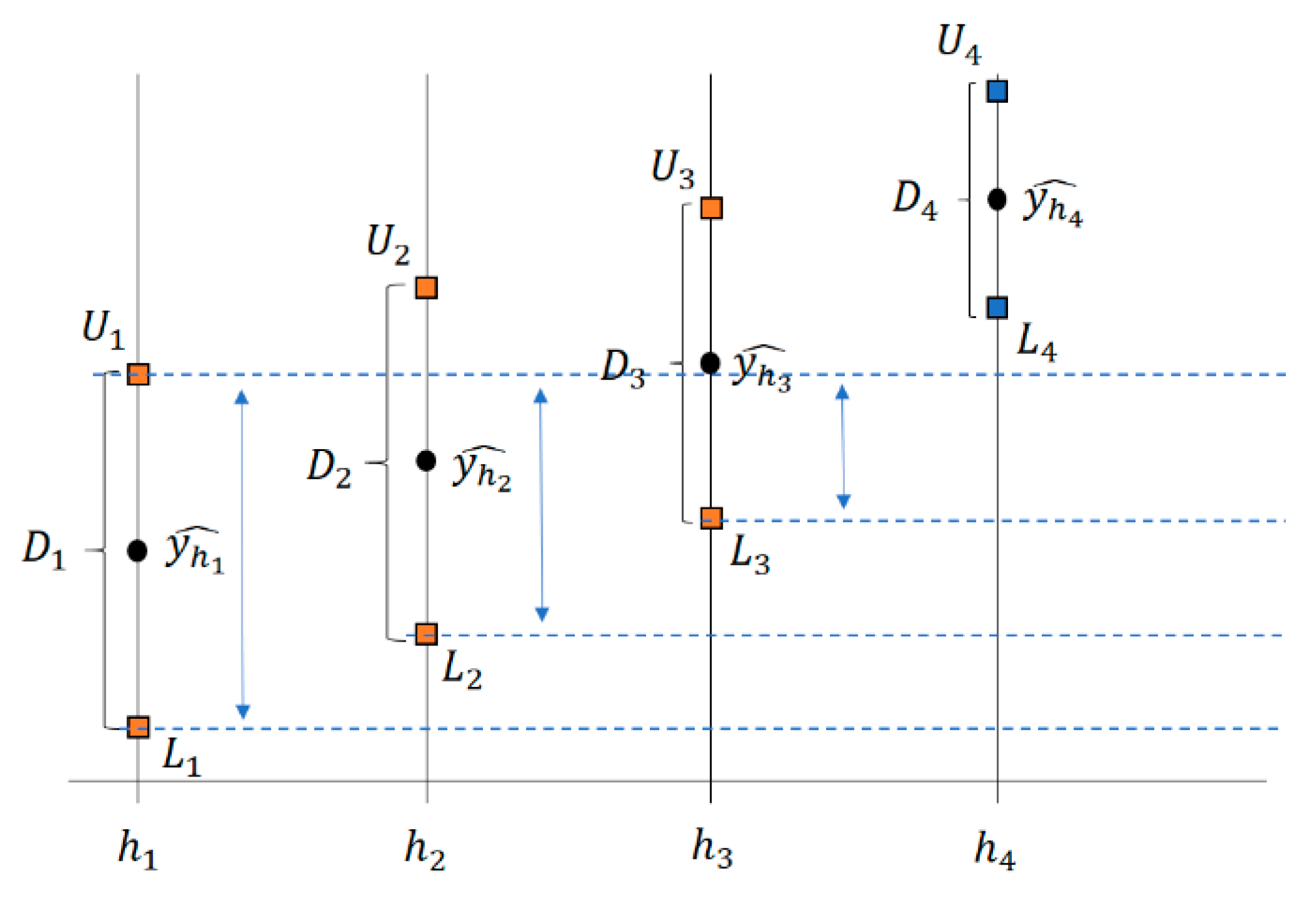
An illustration of tracking of confidence intervals by the ICI algorithm is shown in Figure 1. As it can be seen, the first three confidence intervals have common points, i.e., their intersection is nonempty. On the other hand, is overlapping with and but since it does not overlap with all previous confidence intervals (it is not overlapping with ), the ICI rule results in ℎ3 being chosen as the optimal estimator width.
2.2. The RICI Algorithm
As shown in Equations (2) and (3), the ICI algorithm is highly affected by the selected value of the parameter. Namely, too large values result in oversmoothing (i.e., noise is removed with object edges being blurred) and too small values cause signal undersmoothing (i.e., significant amount of noise is left in the image) [6,7].
Thus, we propose a modification of the ICI rule (further extended to 2D for medical images denoising) shown to be significantly more robust to the suboptimal selections [10,11]. The method is based on tracking the value of the ratio (and thus is called the RICI rule) of the overlapping of the confidence intervals and the length of the current confidence interval, defined as [10,11]:
Next, , given in Equation (15), is then used as an additional criterion for selecting the adaptive filter width [10,11]:
where stands for the preset data-driven threshold value [10,11].
The RICI rule allows selecting larger values (ensuring efficient noise removal), while additional criterion Equation (16) protects from blurring artefacts. Hence, the RICI algorithm smoothes the noise and, at the same time, preserves object contours and edges in the denoised image.
2.3. Extending the ICI and RICI Algorithm to Image Processing
The above described ICI and RICI based algorithms for 1D signal processing were upgraded for detecting two-dimensional regions of interest in the vicinity of the considered image pixel.
Namely, the lower and upper interval limits defined in Equations (2) and (3) were extended to two dimensions (resulting in calculating and ), where i and j define pixel indexes.
The size and the shape of the 2D regions, used in the estimation of the noise-free image pixel, depends on image content and varies from pixel to pixel. Once detected, denoised pixel value is estimated using the 2D LPA based weighted averaging of the pixels in the detected region. The procedure is repeated for each image pixel separately. Namely, in this paper the regions were calculated using two, four and eight lines intersecting in the considered pixel forming quadrilateral, octagonal and hexadecagonal regions, respectively. Examples of adaptive quadrilateral, octagonal and hexadecagonal regions are shown in Figure 2.
The proposed 2D LPA-RICI image denoising method is planned to be published in an extensive virtual instrument together with other methods for image denoising as a part of our future work (as it was case for the ICI and RICI based 1D signal denoising methods made available in [8]).
The next section elaborates on the obtained results in X-ray image denoising.
3. Results and Discussion
This section presents denoising results achieved using the proposed 2D LPA-RICI method applied to three test X-ray images (namely, X-ray scans of shoulder, chest and ankle). The method was implemented in the Matlab 2015b and denoising performances were measured in terms of the peak signal-to-noise ratio (PSNR).
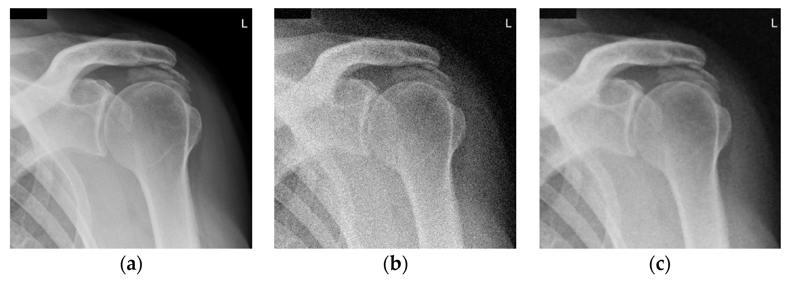
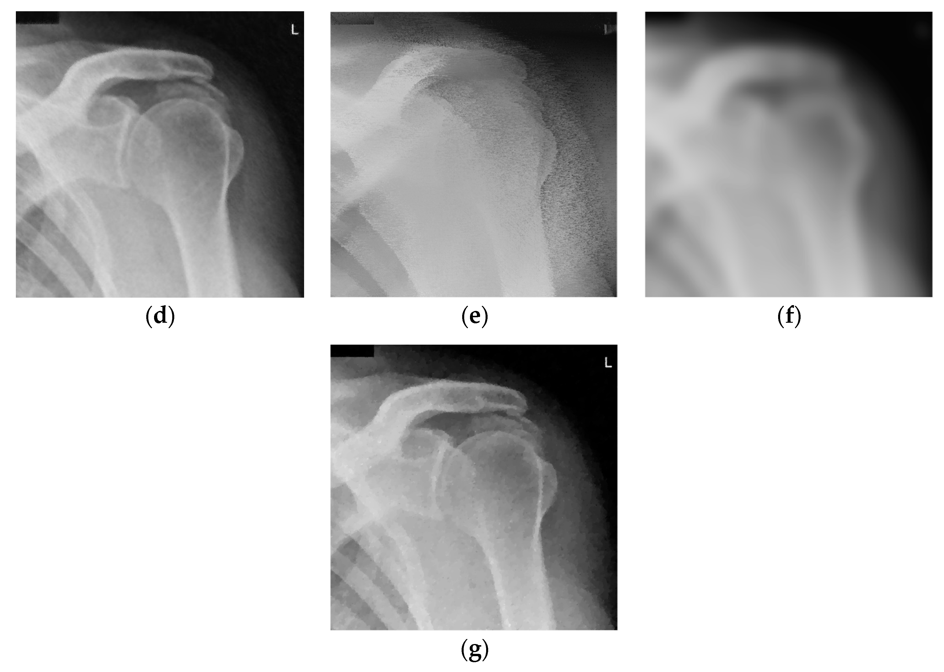
Shoulder X-ray images (with resolution 1024 × 1018) are presented in Figure 3. Namely, the noise-free image is given in Figure 3a. The noisy image is shown in Figure 3b (corrupted by additive white Gaussian noise (AWGN) the standard deviation of which is σ = 25). Figure 3c–e present images denoised using the RICI based method. Namely, Figure 3c is denoised using the quadrilateral regions, Figure 3d is denoised using the octagonal regions and Figure 3e is denoised using the hexadecagonal regions.
Denosing results, in terms of the PSNR, for the shoulder X-ray image are given in Table 1 (for various Г and Rc values). The first column gives regions (octagonal, octagonal and hexadecagonal, respectively). The second and the third column present parameter values for the 2D LPA-RICI denoising method. The fourth column presents the standard deviation of the AWGN. The fifth column provides the noisy image PSNR followed by the column giving the PSNR for image denoised using the proposed RICI based method. The last three columns of the Table 1 show the PSNRs of the images denoised using fixed size filtering (2D median filter), Gaussian smoothing filters and total variation denoising, respectively. For the Gaussian smoothing filtering a Matlab function imgaussfilt was used with standard deviation values chosen same as the standard deviations of the AWGN (σ = 20, 25 and 30). For the total variation denoising [12] Matlab function provided at the MathWorks was used with parameter λ chosen as λ = 0.2, λ = 0.25 and λ = 0.3 for the three tested AWGN levels (σ = 20, 25 and 30), respectively.
Table 2 gives PSNR improvements obtained using the 2D LPA-RICI method vs. noisy image and images denoised using the fixed size filtering, Gaussian smoothing filters and total variation method, respectively. As shown in Table 2, the proposed adaptive RICI based method outperforms the fixed size filters in all cases. Furthermore, it outperforms Gaussian smoothing filters and total variation denoising when quadrilateral and octagonal regions are used (hexadecagonal regions do not outperform Gaussian smoothing and total variation denoising methods).
Namely, the 2D LPA-RICI with quadrilateral regions increased the PSNR of the denoised image by up to 9.13 dB, with octagonal regions increased the PSNR by up to 10.50 dB and with hexadecagonal regions increased the PSNR by up to 4.69 dB (when compared to the noisy image). Also, the proposed 2D LPA-RICI method outperformed the fixed size 2D median filtering by up to 7.99 dB, the Gaussian smoothing filters by up to 6.08 dB and the total variation denoising by up to 4.35 dB for shoulder X-ray scan.
Denoising time for the fixed size filtering was up to 1 s and up to 3 s for the Gaussian smoothing filter and up to 7 min for the total variation denoising. However, the denoising time for the 2D LPA-RICI method without parallelization was up to 40 min for shoulder X-ray scan, depending on the used region. Namely, denoising time for quadrilateral region was up to 24 min, for octagonal region up to 34 min and for hexadecagonal region up to 40 min (greater number of polygonal angles leads to longer execution time).
Denoising of all test images was performed on a personal computer Dell Inspiron 15R 5521 with Intel processor i5 d generation, 6 GB RAM DDR3, 1 TB HDD SATA 1.5 Gbps and Windows 8.1 (64-bit) operating system.
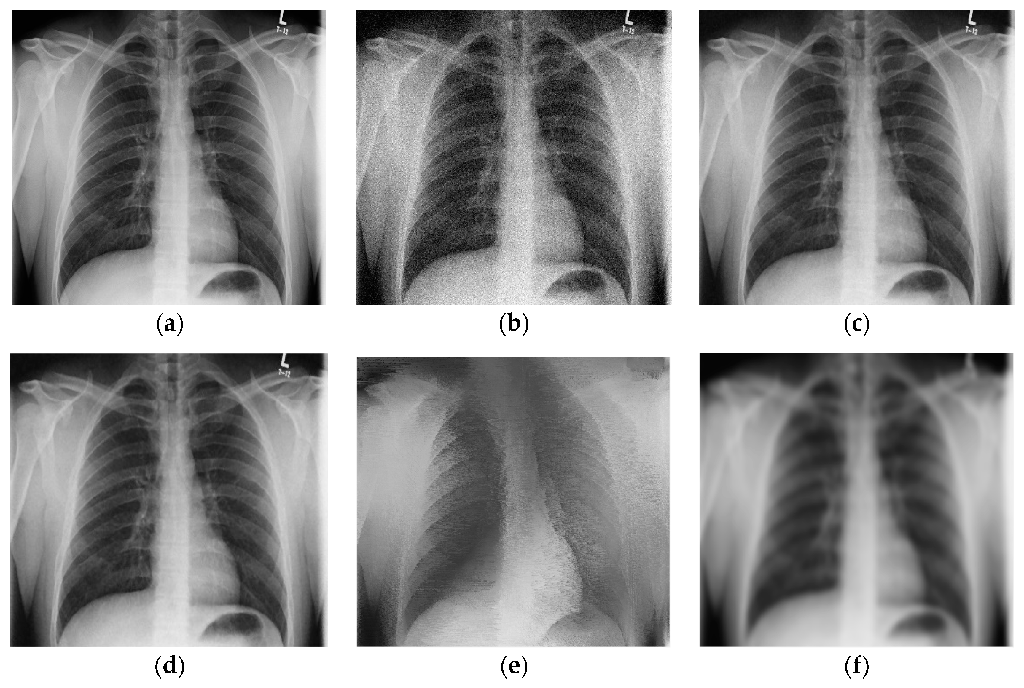
The results for the second test image (chest X-ray image with the resolution 2431 × 1782) are given in Figure 4. Namely, Figure 4a,b shows the noise-free and the noisy image (also corrupted with AWGN with σ = 25), respectively. Figure 4c–e present denoised images obtained using the proposed 2D LPA-RICI algorithm with quadrilateral, octagonal and hexadecagonal regions, respectively.
The PSNR results for denoised chest X-ray images are found in Table 3. As it can be seen from Table 3, the proposed 2D LPA-RICI method (as it was the case for the shoulder X-ray image) outperformed fixed size 2D filtering in all cases. Furthermore, the RICI based denoising outperformed Gaussian smoothing filters and total variation denoising when quadrilateral and octagonal regions were used.
Table 4 gives PSNR improvements for chest X-ray scan denoised using the 2D LAP-RICI method compared to noisy images and images denoised using the fixed size filtering, Gaussian smoothing filters and the total variation method, respectively. Namely, the LPA-RICI method enhanced denoised image quality, both visually and in terms of the PSNR, by up to 9.40 dB when quadrilateral regions were used, by up to 10.23 dB when octagonal regions were used and by up to 5.25 dB when hexadecagonal regions were used (when compared to the noisy image PSNR). It also outperforms fixed size 2D median filtering in all cases, increasing the PSNR by up to 7.51 dB. In addition, the 2D LPA-RICI method outperformed the Gaussian smoothing filters by up to 5.35 dB when quadrilateral and octagonal regions were used. Furthermore, it also outperformed the total variation denoising increasing the PSNR by up to 3.30 dB (in case of the adaptive 2D quadrilateral and octagonal regions).
Denoising time for the chest X-ray scans for the fixed size filtering was up to 1.5 s and for the Gaussian smoothing filter up to 6 s. Furthermore, the denoising time for the total variation method was up to 10.5 min and for the 2D LPA-RICI without parallelization up to 60 min, depending on the used regions (up to 36 min for quadrilateral regions, up to 51 min for octagonal regions and up to 60 min for hexadecagonal regions).
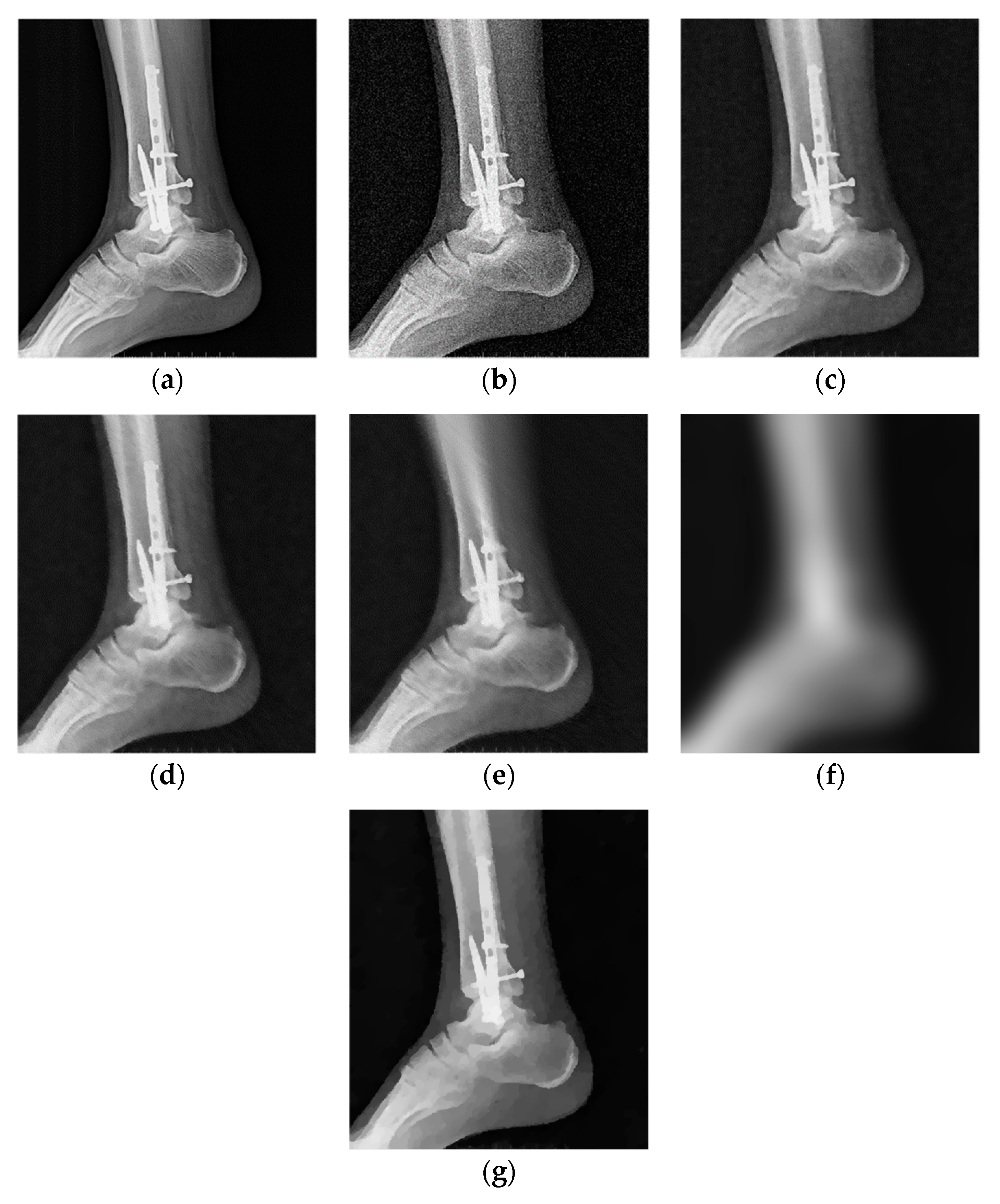
Denoised ankle X-ray images (with resolution 600 × 682) are given in Figure 5. Figure 5a,b show noise-free and noisy images, respectively. Figure 5c–e shows the denoised images obtained using the 2D LPA-RICI method with quadrilateral, octagonal and hexadecagonal regions, respectively.
Table 5 gives the PSNRs of the denoised ankle X-ray images. The proposed 2D LPA-RICI method, as it was the case for other two test images, outperformed fixed size 2D filtering in all cases. Furthermore, it also increased the denoised image PSNR when compared to the Gaussian smoothing filters and the total variation denoising (when quadrilateral or octagonal regions were used).
As it can be seen from Table 6, ankle X-ray scan denoised by the 2D LPA-RICI method with quadrilateral regions resulted in an increased PSNR (compared to the noisy image) by up to 8.09 dB, by up to 7.46 dB with octagonal regions and by up to 3.93 dB with hexadecagonal regions. Once again, the proposed 2D LPA-RICI method was shown to significantly outperform the fixed size 2D median filtering. In addition, it also outperformed Gaussian smoothing filter method for all tested regions (including hexadecagonal regions, which was not the case in the previous examples) by up to 5.46 dB. Furthermore, it increased the denoised PSNR when compared to the total variation denoising method by up to 2.80 dB (when quadrilateral and octagonal regions were used).
Denoising of the ankle X-ray scan took by up to 0.5 s for fixed size filtering, by up to 2 s for the Gaussian smoothing filtering and by up to 5 min for the total variation denoising. Denoising using the LPA-RICI method without parallelization took up to 23 min (for quadrilateral region up to 15.5 min, for octagonal region up to 26 min and for hexadecagonal region up to 32 min).
The provided study showed that the proposed 2D LPA-RICI method performs competitively in terms of medical image denoising due to its adaptivity to image content and calculation of the 2D regions neighbouring the considered pixel for each pixel independently. Furthermore, it was shown that the proposed method outperforms fixed size filters for all tested cases (as shown in Table 1, Table 2, Table 3, Table 4, Table 5 and Table 6). Also, the proposed 2D LPA-RICI method outperforms Gaussian smoothing filters and total variation denoising when adaptive quadrilateral and octagonal regions were used. Furthermore, the obtained results suggest that increasing the number of polygonal angles does not necessarily result in improved estimation accuracy (quadrilateral and octagonal regions performed better than the hexadecagonal regions). However, a larger number of polygonal angles increases computational burden of the 2D LPA-RICI method, thus the study suggests using the 2D LPA-RICI with quadrilateral and octagonal regions in medical imaging applications.
Note also that greater improvements may be obtained in cases of higher resolution images (as it is case for images shown in Figure 3 and Figure 4 compared to the ankle X-ray image in Figure 5).
In addition, since denoising of each image pixel is done independently, the method is applicable for easy parallelization which would reduce its computational expenses.
4. Conclusions
The paper introduces an adaptive denoising method applied to medical image denoising. The proposed method is based on a modification of the ICI algorithm, called the RICI algorithm, extended to local 2D LPA based filtering. The paper shows that the proposed 2D LPA-RICI method performs competitively in terms of medical image denoising due to its adaptivity to image content by readjusting the size and shape of 2D regions from pixel to pixel independently. Thus, the proposed method is easily parallelized for reducing its computational expenses.
The 2D LPA-RICI with quadrilateral, octagonal and hexadecagonal regions was tested in the paper, showing that increasing the number of polygonal angles does not necessarily result in an improved denoising accuracy. On the other hand, a larger number of polynomial angles increases the method’s computational burden.
The method was tested on real-life X-ray images and compared to the fixed size 2D median filtering, Gaussian smoothing filters and the total variation denoising. The 2D LPA-RICI method increased the image PSNR by up to 10.50 dB when compared to the noisy image PSNR. Furthermore, it outperformed the fixed size filtering by up to 7.99 dB, as well as the Gaussian smoothing filters when quadrilateral and octagonal regions were used by up to 6.08 dB. Furthermore, the 2D LPA-RICI method with quadrilateral and octagonal regions outperformed the total variation denoising by up to 4.35 dB.
Acknowledgments
This work has been supported in part by the University of Rijeka under the project number 16.09.2.2.04.
Author Contributions
Ivica Mandić has implemented 2D LPA-RICI method in Matlab and applied it to test images. He contributed in writing draft of the paper as well as in comparing the results obtained by the proposed method to the total variation denoising. Hajdi Peić has implemented adaptive regions (quadrilateral, octagonal and hexadecagonal) in Matlab and analysed PSNRs with respect to tested regions. She also contributed in writing draft of the paper and comparing the results obtained using the proposed method to Gaussian and fixed size filtering. Jonatan Lerga has proposed extending his LPA-RICI method to the 2D LPA-RICI method. He rewrote numerous sections in order to improve the paper’s readability. Furthermore, as a corresponding author, he wrote reply to reviewers’ comments. Ivan Štajduhar contributed in finalizing the revised version of the paper modified according to the reviewers’ suggestions.
Conflicts of Interest
The authors declare no conflict of interest.
References
- Buades, A.; Coll, B.; Morel, J.M. On Image Denoising Methods. CMLA Preprint. 2004, Volume 5. Available online: http://www3.cs.stonybrook.edu/~cse577/image.smoothing.morel.pdf (accessed on 4 February 2018).
- Bansal, M.; Devi, M.; Jain, N.; Kukreja, C. A proposed approach for biomedical image denoising using PCA-NLM. Int. J. Bio-Sci. Bio-Technol. 2014, 6, 13–20. [Google Scholar]
- Samundeeswari, E.S.; Saranya, P.K.; Manavalan, R. M2 filter for speckle noise suppression in breast ultrasound images. ICTACT J. Image Video Process. 2015, 6, 1137–1144. [Google Scholar]
- Vijay, M.; Suhha, S.V.; Karthik, K. Adaptive spatial and wavelet multiscale products thresholding method for medical image denoising. In Proceedings of the International Conference on Computing, Electronics and Electrical Technologies, Kumaracoil, India, 21–22 March 2002; pp. 1109–1114. [Google Scholar]
- Ali, H.M. MRI medical image denoising by fundamental filters. SCIREA J. Comput. 2017, 12, 2–26. [Google Scholar]
- Katkovnik, V.; Egiazarian, K.; Astola, J. A spatially adaptive nonparametric regression image deblurring. IEEE Trans. Image Process. 2005, 14, 1469–1478. [Google Scholar] [CrossRef] [PubMed]
- Katkovnik, V.; Egiazarian, K.; Astola, J. Adaptive window size image de-noising based on intersection of confidence intervals (ICI) rule. J. Math. Imaging Vis. 2002, 16, 223–235. [Google Scholar] [CrossRef]
- Segon, G.; Lerga, J.; Sucic, V. Improved LPA-ICI-based estimators embedded in a signal denoising virtual instrument. Signal Image Video Process. 2017, 11, 211–218. [Google Scholar] [CrossRef]
- Katkovnik, V.; Egiazarian, K.; Astola, J. Local Approximation Techniques in Signal and Image Processing; SPIE Publications—The International Society for Optical Engineering: Washington, WA, USA, 2006. [Google Scholar]
- Lerga, J.; Vrankic, M.; Sucic, V. A signal denoising method based on the improved ICI rule. IEEE Signal Process. Lett. 2008, 15, 601–604. [Google Scholar] [CrossRef]
- Lerga, J.; Sucic, V.; Grbac, E. An adaptive method for video denoising based on the ICI rule. Eng. Rev. 2012, 32, 33–40. [Google Scholar]
- Rudin, L.I.; Osher, S.; Fatemi, E. Nonlinear total variation based noise removal algorithms. Phys. D Nonlinear Phenom. 1992, 60, 259–268. [Google Scholar] [CrossRef]
Figure 1.
Illustration of the ICI rule tracking the intersection of the confidence intervals.

Figure 2.
Examples of the detected regions obtained using the proposed method. (a) Quadrilateral region; (b) Octagonal region; (c) Hexadecagonal region.
Figure 2.
Examples of the detected regions obtained using the proposed method. (a) Quadrilateral region; (b) Octagonal region; (c) Hexadecagonal region.
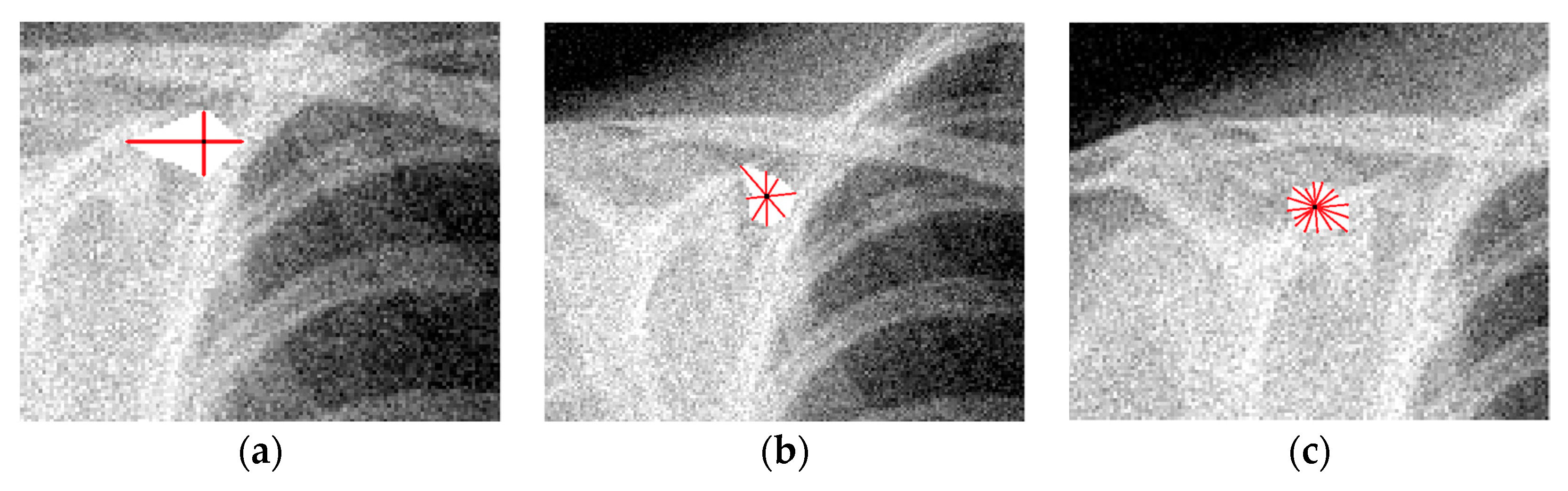
Figure 3.
Shoulder X-ray scan. (a) Original noise-free image; (b) Noisy image (AWGN with σ = 25); (c) Image denoised using the 2D LPA-RICI method (quadrilateral region, Г = 1.8, Rc = 0.8); (d) Image denoised using the 2D LPA-RICI method (octagonal region, Г = 1.8, Rc = 0.8); (e) Image denoised using the 2D LPA-RICI method (hexadecagonal region, Г = 1.8, Rc = 0.8); (f) Image denoised using Gaussian smoothing filters; (g) Image denoised using total variation denoising.


Figure 4.
Chest X-ray scan. (a) Original noise-free image; (b) Noisy image (AWGN with σ = 25); (c) Image denoised using the 2D LPA-RICI method (quadrilateral region, Г = 1.8, Rc = 0.8); (d) Image denoised using the 2D LPA-RICI method (octagonal region, Г = 1.8, Rc = 0.8); (e) Image denoised using the 2D LPA-RICI method (hexadecagonal region, Г = 1.8, Rc = 0.8); (f) Image denoised using Gaussian smoothing filters; (g) Image denoised using total variation denoising.

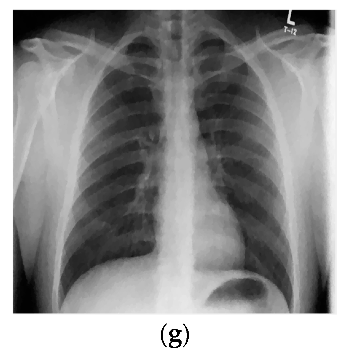
Figure 5.
Ankle X-ray scan. (a) Original noise-free image; (b) Noisy image (AWGN with σ = 25); (c) Image denoised using the 2D LPA-RICI method (quadrilateral region, Г = 1.8, Rc = 0.8); (d) Image denoised using the 2D LPA-RICI method (octagonal region, Г = 1.8, Rc = 0.8); (e) Image denoised using the 2D LPA-RICI method (hexadecagonal region, Г = 1.8, Rc = 0.8); (f) Image denoised using Gaussian smoothing filters; (g) Image denoised using total variation denoising.


Table 1.
PSNRs for shoulder X-ray images denoised using the proposed 2D LPA-RICI method and competitive methods.
Table 1.
PSNRs for shoulder X-ray images denoised using the proposed 2D LPA-RICI method and competitive methods.
| Parameters | PSNR (dB) | |||||||
|---|---|---|---|---|---|---|---|---|
| Region | Г | Rc | σ | Noisy Image | RICI | Fixed Size Filters | Gaussian Smoothing | Total Variation |
| Quadrilateral | 1.8 | 0.8 | 20 | 29.82 | 38.73 | 33.4 | 34.69 | 35.02 |
| Octagonal | 1.8 | 0.8 | 20 | 29.82 | 39.37 | 33.4 | 34.69 | 35.02 |
| Hexadecagonal | 1.8 | 0.8 | 20 | 29.82 | 33.61 | 33.4 | 34.69 | 35.02 |
| Quadrilateral | 1.7 | 0.9 | 20 | 29.82 | 38.63 | 33.4 | 34.69 | 35.02 |
| Octagonal | 1.7 | 0.9 | 20 | 29.82 | 39.1 | 33.4 | 34.69 | 35.02 |
| Hexadecagonal | 1.7 | 0.9 | 20 | 29.82 | 33.42 | 33.4 | 34.69 | 35.02 |
| Quadrilateral | 1.6 | 0.6 | 20 | 29.82 | 38.72 | 33.4 | 34.69 | 35.02 |
| Octagonal | 1.6 | 0.6 | 20 | 29.82 | 39.19 | 33.4 | 34.69 | 35.02 |
| Hexadecagonal | 1.6 | 0.6 | 20 | 29.82 | 33.5 | 33.4 | 34.69 | 35.02 |
| Quadrilateral | 1.8 | 0.8 | 25 | 29.32 | 38.45 | 32.24 | 33.99 | 36.69 |
| Octagonal | 1.8 | 0.8 | 25 | 29.32 | 38.96 | 32.34 | 33.99 | 36.69 |
| Hexadecagonal | 1.8 | 0.8 | 25 | 29.32 | 33.51 | 32.34 | 33.99 | 36.69 |
| Quadrilateral | 1.7 | 0.9 | 25 | 29.32 | 38.17 | 32.24 | 33.99 | 36.69 |
| Octagonal | 1.7 | 0.9 | 25 | 29.32 | 38.82 | 32.24 | 33.99 | 36.69 |
| Hexadecagonal | 1.7 | 0.9 | 25 | 29.32 | 33.5 | 32.24 | 33.99 | 36.69 |
| Quadrilateral | 1.6 | 0.6 | 25 | 29.32 | 38.27 | 32.24 | 33.99 | 36.69 |
| Octagonal | 1.6 | 0.6 | 25 | 29.32 | 38.84 | 32.24 | 33.99 | 36.69 |
| Hexadecagonal | 1.6 | 0.6 | 25 | 29.32 | 33.57 | 32.24 | 33.99 | 36.69 |
| Quadrilateral | 1.8 | 0.8 | 30 | 28.99 | 38.09 | 31.5 | 33.41 | 35.62 |
| Octagonal | 1.8 | 0.8 | 30 | 28.99 | 38.76 | 31.5 | 33.41 | 35.62 |
| Hexadecagonal | 1.8 | 0.8 | 30 | 28.99 | 33.68 | 31.5 | 33.41 | 35.62 |
| Quadrilateral | 1.7 | 0.9 | 30 | 28.99 | 37.78 | 31.5 | 33.41 | 35.62 |
| Octagonal | 1.7 | 0.9 | 30 | 28.99 | 38.58 | 31.5 | 33.41 | 35.62 |
| Hexadecagonal | 1.7 | 0.9 | 30 | 28.99 | 33.4 | 31.5 | 33.41 | 35.62 |
| Quadrilateral | 1.6 | 0.6 | 30 | 28.99 | 37.82 | 31.5 | 33.41 | 35.62 |
| Octagonal | 1.6 | 0.6 | 30 | 28.99 | 39.49 | 31.5 | 33.41 | 35.62 |
| Hexadecagonal | 1.6 | 0.6 | 30 | 28.99 | 33.66 | 31.5 | 33.41 | 35.62 |
Table 2.
PSNR improvements for shoulder X-ray images denoised using the proposed 2D LPA-RICI method vs. the competitive methods.
Table 2.
PSNR improvements for shoulder X-ray images denoised using the proposed 2D LPA-RICI method vs. the competitive methods.
| Parameters | PSNR (dB) | ||||||
|---|---|---|---|---|---|---|---|
| Region | Г | Rc | σ | RICI vs. Noisy | RICI vs. Fixed | RICI vs. GAUSSIAN | RICI vs. Total Variation |
| Quadrilateral | 1.8 | 0.8 | 20 | 8.91 | 5.33 | 4.04 | 3.71 |
| Octagonal | 1.8 | 0.8 | 20 | 9.55 | 5.97 | 4.68 | 4.35 |
| Hexadecagonal | 1.8 | 0.8 | 20 | 3.79 | 0.21 | −1.08 | −1.41 |
| Quadrilateral | 1.7 | 0.9 | 20 | 8.81 | 5.23 | 3.94 | 3.61 |
| Octagonal | 1.7 | 0.9 | 20 | 9.28 | 5.7 | 4.41 | 4.08 |
| Hexadecagonal | 1.7 | 0.9 | 20 | 3.6 | 0.02 | −1.27 | −1.6 |
| Quadrilateral | 1.6 | 0.6 | 20 | 8.9 | 5.32 | 4.03 | 3.7 |
| Octagonal | 1.6 | 0.6 | 20 | 9.37 | 5.79 | 4.5 | 4.17 |
| Hexadecagonal | 1.6 | 0.6 | 20 | 3.68 | 0.1 | −1.19 | −1.52 |
| Quadrilateral | 1.8 | 0.8 | 25 | 9.13 | 6.21 | 4.46 | 1.76 |
| Octagonal | 1.8 | 0.8 | 25 | 9.64 | 6.62 | 4.97 | 2.27 |
| Hexadecagonal | 1.8 | 0.8 | 25 | 4.19 | 1.17 | −0.48 | −3.18 |
| Quadrilateral | 1.7 | 0.9 | 25 | 8.85 | 5.93 | 4.18 | 1.48 |
| Octagonal | 1.7 | 0.9 | 25 | 9.5 | 6.58 | 4.83 | 2.13 |
| Hexadecagonal | 1.7 | 0.9 | 25 | 4.18 | 1.26 | −0.49 | −3.19 |
| Quadrilateral | 1.6 | 0.6 | 25 | 8.95 | 6.03 | 4.28 | 1.58 |
| Octagonal | 1.6 | 0.6 | 25 | 9.52 | 6.6 | 4.85 | 2.15 |
| Hexadecagonal | 1.6 | 0.6 | 25 | 4.25 | 1.33 | −0.42 | −3.12 |
| Quadrilateral | 1.8 | 0.8 | 30 | 9.1 | 6.59 | 4.68 | 2.47 |
| Octagonal | 1.8 | 0.8 | 30 | 9.77 | 7.26 | 5.35 | 3.14 |
| Hexadecagonal | 1.8 | 0.8 | 30 | 4.69 | 2.18 | 0.27 | −1.94 |
| Quadrilateral | 1.7 | 0.9 | 30 | 8.79 | 6.28 | 4.37 | 2.16 |
| Octagonal | 1.7 | 0.9 | 30 | 9.59 | 7.08 | 5.17 | 2.96 |
| Hexadecagonal | 1.7 | 0.9 | 30 | 4.41 | 1.9 | −0.01 | −2.22 |
| Quadrilateral | 1.6 | 0.6 | 30 | 8.83 | 6.32 | 4.41 | 2.2 |
| Octagonal | 1.6 | 0.6 | 30 | 10.5 | 7.99 | 6.08 | 3.87 |
| Hexadecagonal | 1.6 | 0.6 | 30 | 4.67 | 2.16 | 0.25 | −1.96 |
Table 3.
PSNRs for chest X-ray images denoised using the proposed 2D LPA-RICI method and the competitive methods.
Table 3.
PSNRs for chest X-ray images denoised using the proposed 2D LPA-RICI method and the competitive methods.
| Parameters | PSNR (dB) | |||||||
|---|---|---|---|---|---|---|---|---|
| Region | Г | Rc | σ | Noisy Image | RICI | Fixed Size Filters | Gaussian Smoothing | Total Variation |
| Quadrilateral | 1.8 | 0.8 | 20 | 29.36 | 36.8 | 33.23 | 34.18 | 35.34 |
| Octagonal | 1.8 | 0.8 | 20 | 29.36 | 38.09 | 33.23 | 34.18 | 35.34 |
| Hexadecagonal | 1.8 | 0.8 | 20 | 29.36 | 33.76 | 33.23 | 34.18 | 35.34 |
| Quadrilateral | 1.7 | 0.9 | 20 | 29.36 | 36.74 | 33.23 | 34.18 | 35.34 |
| Octagonal | 1.7 | 0.9 | 20 | 29.36 | 38.23 | 33.23 | 34.18 | 35.34 |
| Hexadecagonal | 1.7 | 0.9 | 20 | 29.36 | 33.81 | 33.23 | 34.18 | 35.34 |
| Quadrilateral | 1.6 | 0.6 | 20 | 29.36 | 36.6 | 33.23 | 34.18 | 35.34 |
| Octagonal | 1.6 | 0.6 | 20 | 29.36 | 38.06 | 33.23 | 34.18 | 35.34 |
| Hexadecagonal | 1.6 | 0.6 | 20 | 29.36 | 33.3 | 33.23 | 34.18 | 35.34 |
| Quadrilateral | 1.8 | 0.8 | 25 | 28.26 | 37.28 | 31.86 | 33.76 | 36.43 |
| Octagonal | 1.8 | 0.8 | 25 | 28.26 | 38.49 | 31.86 | 33.76 | 36.43 |
| Hexadecagonal | 1.8 | 0.8 | 25 | 28.26 | 33.51 | 31.86 | 33.76 | 36.43 |
| Quadrilateral | 1.7 | 0.9 | 25 | 28.26 | 37.66 | 31.86 | 33.76 | 36.43 |
| Octagonal | 1.7 | 0.9 | 25 | 28.26 | 38.47 | 31.86 | 33.76 | 36.43 |
| Hexadecagonal | 1.7 | 0.9 | 25 | 28.26 | 32.58 | 31.86 | 33.76 | 36.43 |
| Quadrilateral | 1.6 | 0.6 | 25 | 28.26 | 37.26 | 31.86 | 33.76 | 36.43 |
| Octagonal | 1.6 | 0.6 | 25 | 28.26 | 38.48 | 31.86 | 33.76 | 36.43 |
| Hexadecagonal | 1.6 | 0.6 | 25 | 28.26 | 33.09 | 31.86 | 33.76 | 36.43 |
| Quadrilateral | 1.8 | 0.8 | 30 | 28.87 | 37.74 | 31.01 | 33.17 | 35.22 |
| Octagonal | 1.8 | 0.8 | 30 | 28.87 | 38.47 | 31.01 | 33.17 | 35.22 |
| Hexadecagonal | 1.8 | 0.8 | 30 | 28.87 | 33.01 | 31.01 | 33.17 | 35.22 |
| Quadrilateral | 1.7 | 0.9 | 30 | 28.87 | 36.96 | 31.01 | 33.17 | 35.22 |
| Octagonal | 1.7 | 0.9 | 30 | 28.87 | 38.52 | 31.01 | 33.17 | 35.22 |
| Hexadecagonal | 1.7 | 0.9 | 30 | 28.87 | 33.14 | 31.01 | 33.17 | 35.22 |
| Quadrilateral | 1.6 | 0.6 | 30 | 28.87 | 37.62 | 31.01 | 33.17 | 35.22 |
| Octagonal | 1.6 | 0.6 | 30 | 28.87 | 37.94 | 31.01 | 33.17 | 35.22 |
| Hexadecagonal | 1.6 | 0.6 | 30 | 28.87 | 32.92 | 31.01 | 33.17 | 35.22 |
Table 4.
PSNR improvements for chest X-ray images denoised using the proposed 2D LPA-RICI method vs. the competitive methods.
Table 4.
PSNR improvements for chest X-ray images denoised using the proposed 2D LPA-RICI method vs. the competitive methods.
| Parameters | PSNR (dB) | ||||||
|---|---|---|---|---|---|---|---|
| Region | Г | Rc | σ | RICI vs. Noisy | RICI vs. Fixed | RICI vs. Gaussian | RICI vs. Total Variation |
| Quadrilateral | 1.8 | 0.8 | 20 | 7.44 | 3.57 | 2.62 | 1.46 |
| Octagonal | 1.8 | 0.8 | 20 | 8.73 | 4.86 | 3.91 | 2.75 |
| Hexadecagonal | 1.8 | 0.8 | 20 | 4.4 | 0.53 | −0.42 | −1.58 |
| Quadrilateral | 1.7 | 0.9 | 20 | 7.38 | 3.51 | 2.56 | 1.4 |
| Octagonal | 1.7 | 0.9 | 20 | 8.87 | 5 | 4.05 | 2.89 |
| Hexadecagonal | 1.7 | 0.9 | 20 | 4.45 | 0.58 | −0.37 | −1.53 |
| Quadrilateral | 1.6 | 0.6 | 20 | 7.24 | 3.37 | 2.42 | 1.26 |
| Octagonal | 1.6 | 0.6 | 20 | 8.7 | 4.83 | 3.88 | 2.72 |
| Hexadecagonal | 1.6 | 0.6 | 20 | 3.94 | 0.07 | −0.88 | −2.04 |
| Quadrilateral | 1.8 | 0.8 | 25 | 9.02 | 5.42 | 3.52 | 0.85 |
| Octagonal | 1.8 | 0.8 | 25 | 10.23 | 6.63 | 4.73 | 2.06 |
| Hexadecagonal | 1.8 | 0.8 | 25 | 5.25 | 1.65 | −0.25 | −2.92 |
| Quadrilateral | 1.7 | 0.9 | 25 | 9.4 | 5.8 | 3.9 | 1.23 |
| Octagonal | 1.7 | 0.9 | 25 | 10.21 | 6.61 | 4.71 | 2.04 |
| Hexadecagonal | 1.7 | 0.9 | 25 | 4.32 | 0.72 | −1.18 | −3.85 |
| Quadrilateral | 1.6 | 0.6 | 25 | 9 | 5.4 | 3.5 | 0.83 |
| Octagonal | 1.6 | 0.6 | 25 | 10.22 | 6.62 | 4.72 | 2.05 |
| Hexadecagonal | 1.6 | 0.6 | 25 | 4.83 | 1.23 | −0.67 | −3.34 |
| Quadrilateral | 1.8 | 0.8 | 30 | 8.87 | 6.73 | 4.57 | 2.52 |
| Octagonal | 1.8 | 0.8 | 30 | 9.6 | 7.46 | 5.3 | 3.25 |
| Hexadecagonal | 1.8 | 0.8 | 30 | 4.14 | 2 | −0.16 | −2.21 |
| Quadrilateral | 1.7 | 0.9 | 30 | 8.09 | 5.95 | 3.79 | 1.74 |
| Octagonal | 1.7 | 0.9 | 30 | 9.65 | 7.51 | 5.35 | 3.3 |
| Hexadecagonal | 1.7 | 0.9 | 30 | 4.27 | 2.13 | −0.03 | −2.08 |
| Quadrilateral | 1.6 | 0.6 | 30 | 8.75 | 6.61 | 4.45 | 2.4 |
| Octagonal | 1.6 | 0.6 | 30 | 9.07 | 6.93 | 4.77 | 2.72 |
| Hexadecagonal | 1.6 | 0.6 | 30 | 4.05 | 1.91 | −0.25 | −2.3 |
Table 5.
PSNRs for ankle X-ray images denoised using the proposed 2D LPA-RICI method and the competitive methods.
Table 5.
PSNRs for ankle X-ray images denoised using the proposed 2D LPA-RICI method and the competitive methods.
| Parameters | PSNR (dB) | |||||||
|---|---|---|---|---|---|---|---|---|
| Region | Г | Rc | σ | Noisy Image | RICI | Fixed Size Filters | Gaussian Smoothing | Total Variation |
| Quadrilateral | 1.8 | 0.8 | 20 | 29.85 | 36.68 | 32.79 | 32.22 | 34.45 |
| Octagonal | 1.8 | 0.8 | 20 | 29.85 | 36.16 | 32.79 | 32.22 | 34.45 |
| Hexadecagonal | 1.8 | 0.8 | 20 | 29.85 | 32.92 | 32.79 | 32.22 | 34.45 |
| Quadrilateral | 1.7 | 0.9 | 20 | 29.85 | 36.97 | 32.79 | 32.22 | 34.45 |
| Octagonal | 1.7 | 0.9 | 20 | 29.85 | 36.28 | 32.79 | 32.22 | 34.45 |
| Hexadecagonal | 1.7 | 0.9 | 20 | 29.85 | 32.83 | 32.79 | 32.22 | 34.45 |
| Quadrilateral | 1.6 | 0.6 | 20 | 29.85 | 36.93 | 32.79 | 32.22 | 34.45 |
| Octagonal | 1.6 | 0.6 | 20 | 29.85 | 36.41 | 32.79 | 32.22 | 34.45 |
| Hexadecagonal | 1.6 | 0.6 | 20 | 29.85 | 32.95 | 32.79 | 32.22 | 34.45 |
| Quadrilateral | 1.8 | 0.8 | 25 | 29.37 | 37.23 | 31.96 | 31.93 | 35.61 |
| Octagonal | 1.8 | 0.8 | 25 | 29.37 | 36.57 | 31.96 | 31.93 | 35.61 |
| Hexadecagonal | 1.8 | 0.8 | 25 | 29.37 | 32.94 | 31.96 | 31.93 | 35.61 |
| Quadrilateral | 1.7 | 0.9 | 25 | 29.37 | 37.07 | 31.96 | 31.93 | 35.61 |
| Octagonal | 1.7 | 0.9 | 25 | 29.37 | 36.67 | 31.96 | 31.93 | 35.61 |
| Hexadecagonal | 1.7 | 0.9 | 25 | 29.37 | 32.98 | 31.96 | 31.93 | 35.61 |
| Quadrilateral | 1.6 | 0.6 | 25 | 29.37 | 37.03 | 31.96 | 31.93 | 35.61 |
| Octagonal | 1.6 | 0.6 | 25 | 29.37 | 36.83 | 31.96 | 31.93 | 35.61 |
| Hexadecagonal | 1.6 | 0.6 | 25 | 29.37 | 32.98 | 31.96 | 31.93 | 35.61 |
| Quadrilateral | 1.8 | 0.8 | 30 | 29.06 | 37.15 | 31.15 | 31.69 | 34.35 |
| Octagonal | 1.8 | 0.8 | 30 | 29.06 | 36.35 | 31.15 | 31.69 | 34.35 |
| Hexadecagonal | 1.8 | 0.8 | 30 | 29.06 | 32.63 | 31.15 | 31.69 | 34.35 |
| Quadrilateral | 1.7 | 0.9 | 30 | 29.06 | 36.97 | 31.15 | 31.69 | 34.35 |
| Octagonal | 1.7 | 0.9 | 30 | 29.06 | 36.28 | 31.15 | 31.69 | 34.35 |
| Hexadecagonal | 1.7 | 0.9 | 30 | 29.06 | 32.83 | 31.15 | 31.69 | 34.35 |
| Quadrilateral | 1.6 | 0.6 | 30 | 29.06 | 37.11 | 31.15 | 31.69 | 34.35 |
| Octagonal | 1.6 | 0.6 | 30 | 29.06 | 36.51 | 31.15 | 31.69 | 34.35 |
| Hexadecagonal | 1.6 | 0.6 | 30 | 29.06 | 32.99 | 31.15 | 31.69 | 34.35 |
Table 6.
PSNR improvements for ankle X-ray images denoised using the proposed 2D LPA-RICI method vs. the competitive methods.
Table 6.
PSNR improvements for ankle X-ray images denoised using the proposed 2D LPA-RICI method vs. the competitive methods.
| Parameters | PSNR (dB) | ||||||
|---|---|---|---|---|---|---|---|
| Region | Г | Rc | σ | RICI vs. Noisy | RICI vs. Fixed | RICI vs. Gaussian | RICI vs. Total Variation |
| Quadrilateral | 1.8 | 0.8 | 20 | 6.83 | 3.89 | 4.46 | 2.23 |
| Octagonal | 1.8 | 0.8 | 20 | 6.31 | 3.37 | 3.94 | 1.71 |
| Hexadecagonal | 1.8 | 0.8 | 20 | 3.07 | 0.13 | 0.70 | −1.53 |
| Quadrilateral | 1.7 | 0.9 | 20 | 7.12 | 4.18 | 4.75 | 2.52 |
| Octagonal | 1.7 | 0.9 | 20 | 6.43 | 3.49 | 4.06 | 1.83 |
| Hexadecagonal | 1.7 | 0.9 | 20 | 2.98 | 0.04 | 0.61 | −1.62 |
| Quadrilateral | 1.6 | 0.6 | 20 | 7.08 | 4.14 | 4.71 | 2.48 |
| Octagonal | 1.6 | 0.6 | 20 | 6.56 | 3.62 | 4.19 | 1.96 |
| Hexadecagonal | 1.6 | 0.6 | 20 | 3.10 | 0.16 | 0.73 | −1.50 |
| Quadrilateral | 1.8 | 0.8 | 25 | 7.86 | 5.27 | 5.30 | 1.62 |
| Octagonal | 1.8 | 0.8 | 25 | 7.20 | 4.61 | 4.64 | 0.96 |
| Hexadecagonal | 1.8 | 0.8 | 25 | 3.57 | 0.98 | 1.01 | −2.67 |
| Quadrilateral | 1.7 | 0.9 | 25 | 7.70 | 5.11 | 5.14 | 1.46 |
| Octagonal | 1.7 | 0.9 | 25 | 7.30 | 4.71 | 4.74 | 1.06 |
| Hexadecagonal | 1.7 | 0.9 | 25 | 3.61 | 1.02 | 1.05 | −2.63 |
| Quadrilateral | 1.6 | 0.6 | 25 | 7.66 | 5.07 | 5.10 | 1.42 |
| Octagonal | 1.6 | 0.6 | 25 | 7.46 | 4.87 | 4.90 | 1.22 |
| Hexadecagonal | 1.6 | 0.6 | 25 | 3.61 | 1.02 | 1.05 | −2.63 |
| Quadrilateral | 1.8 | 0.8 | 30 | 8.09 | 6.00 | 5.46 | 2.80 |
| Octagonal | 1.8 | 0.8 | 30 | 7.29 | 5.20 | 4.66 | 2.00 |
| Hexadecagonal | 1.8 | 0.8 | 30 | 3.57 | 1.48 | 0.94 | −1.72 |
| Quadrilateral | 1.7 | 0.9 | 30 | 7.91 | 5.82 | 5.28 | 2.62 |
| Octagonal | 1.7 | 0.9 | 30 | 7.22 | 5.13 | 4.59 | 1.93 |
| Hexadecagonal | 1.7 | 0.9 | 30 | 3.77 | 1.68 | 1.14 | −1.52 |
| Quadrilateral | 1.6 | 0.6 | 30 | 8.05 | 5.96 | 5.42 | 2.76 |
| Octagonal | 1.6 | 0.6 | 30 | 7.45 | 5.36 | 4.82 | 2.16 |
| Hexadecagonal | 1.6 | 0.6 | 30 | 3.93 | 1.84 | 1.30 | −1.36 |
© 2018 by the authors. Licensee MDPI, Basel, Switzerland. This article is an open access article distributed under the terms and conditions of the Creative Commons Attribution (CC BY) license (http://creativecommons.org/licenses/by/4.0/).
Share and Cite
MDPI and ACS Style
Mandić, I.; Peić, H.; Lerga, J.; Štajduhar, I. Denoising of X-ray Images Using the Adaptive Algorithm Based on the LPA-RICI Algorithm. J. Imaging 2018, 4, 34. https://doi.org/10.3390/jimaging4020034
AMA Style
Mandić I, Peić H, Lerga J, Štajduhar I. Denoising of X-ray Images Using the Adaptive Algorithm Based on the LPA-RICI Algorithm. Journal of Imaging. 2018; 4(2):34. https://doi.org/10.3390/jimaging4020034
Chicago/Turabian StyleMandić, Ivica, Hajdi Peić, Jonatan Lerga, and Ivan Štajduhar. 2018. "Denoising of X-ray Images Using the Adaptive Algorithm Based on the LPA-RICI Algorithm" Journal of Imaging 4, no. 2: 34. https://doi.org/10.3390/jimaging4020034
Note that from the first issue of 2016, this journal uses article numbers instead of page numbers. See further details here.