Handwritten Devanagari Character Recognition Using Layer-Wise Training of Deep Convolutional Neural Networks and Adaptive Gradient Methods


1
Department of Computer Science and Engineering, School of Computing & Information Technology, Manipal University Jaipur, Rajasthan 303007, India
2
Department of Information Technology, School of Computing & Information Technology, Manipal University Jaipur, Rajasthan 303007, India
*
Author to whom correspondence should be addressed.
J. Imaging 2018, 4(2), 41; https://doi.org/10.3390/jimaging4020041
Submission received: 6 December 2017
/
Revised: 9 February 2018
/
Accepted: 12 February 2018
/
Published: 13 February 2018
(This article belongs to the Special Issue Document Image Processing)
Abstract
:Handwritten character recognition is currently getting the attention of researchers because of possible applications in assisting technology for blind and visually impaired users, human–robot interaction, automatic data entry for business documents, etc. In this work, we propose a technique to recognize handwritten Devanagari characters using deep convolutional neural networks (DCNN) which are one of the recent techniques adopted from the deep learning community. We experimented the ISIDCHAR database provided by (Information Sharing Index) ISI, Kolkata and V2DMDCHAR database with six different architectures of DCNN to evaluate the performance and also investigate the use of six recently developed adaptive gradient methods. A layer-wise technique of DCNN has been employed that helped to achieve the highest recognition accuracy and also get a faster convergence rate. The results of layer-wise-trained DCNN are favorable in comparison with those achieved by a shallow technique of handcrafted features and standard DCNN.
1. Introduction
In the last few years, deep learning approaches [1] have been successfully applied to various areas such as image classification, speech recognition, cancer cell detection, video search, face detection, satellite imagery, recognizing traffic signs and pedestrian detection, etc. The outcome of deep learning approaches is also prominent, and in some cases the results are superior to human experts [2,3] in the past years. Most of the problems are also being re-experimented with deep learning approaches with the view to achieving improvements in the existing findings. Different architectures of deep learning have been introduced in recent years, such as deep convolutional neural networks, deep belief networks, and recurrent neural networks. The entire architecture has shown the proficiency in different areas. Character recognition is one of the areas where machine learning techniques have been extensively experimented. The first deep learning approach, which is one of the leading machine learning techniques, was proposed for character recognition in 1998 on MNIST database [4]. The deep learning techniques are basically composed of multiple hidden layers, and each hidden layer consists of multiple neurons, which compute the suitable weights for the deep network. A lot of computing power is needed to compute these weights, and a powerful system was needed, which was not easily available at that time. Since then, the researchers have drawn their attention to finding the technique which needs less power by converting the images into feature vectors. In the last few decades, a lot of feature extraction techniques have been proposed such as HOG (histogram of oriented gradients) [5], SIFT (scale-invariant feature transform) [6,7], LBP (local binary pattern) [8] and SURF (speeded up robust features) [9]. These are prominent feature extraction methods, which have been experimented for many problems like image recognition, character recognition, face detection, etc. and the corresponding models are called shallow learning models, which are still popular for the pattern recognition. Feature extraction [10] is one type of dimensionality reduction technique that represents the important parts of a large image into a feature vector. These features are handcrafted and explicitly designed by the research community. The robustness and performance of these features depend on the skill and the knowledge of each researcher. There are the cases where some vital features may be unseen by the researchers while extracting the features from the image and this may result in a high classification error.
Deep learning inverts the process of handcrafting and designing features for a particular problem into an automatic process to compute the best features for that problem. A deep convolutional neural network has multiple convolutional layers to extract the features automatically. The features are extracted only once in most of the shallow learning models, but in the case of deep learning models, multiple convolutional layers have been adopted to extract discriminating features multiple times. This is one of the reasons that deep learning models are generally successful. The LeNet [4] is an example of deep convolutional neural network for character recognition. Recently, many other examples of deep learning models can be listed such as AlexNet [3], ZFNet [11], VGGNet [12] and spatial transformer networks [13]. These models have been successfully applied for image classification and character recognition. Owing to their great success, many leading companies have also introduced deep models. Google Corporation has made a GoogLeNet having 22 layers of convolutional and pooling layers alternatively. Apart from this model, Google has also developed an open source software library named Tensorflow to conduct deep learning research. Microsoft also introduced its own deep convolutional neural network architecture named ResNet in 2015. ResNet has 152-layer network architectures which made a new record in detection, localization, and classification. This model introduced a new idea of residual learning that makes the optimization and the back-propagation process easier than the basic DCNN model.
Character recognition is a field of image processing where the image is recognized and converted into a machine-readable format. As discussed above, the deep learning approach and especially deep convolutional neural networks have been used for image detection and recognition. It has also been successfully applied on Roman (MNIST) [4], Chinese [14], Bangla [15] and Arabic [16] languages. In this work, a deep convolutional neural network is applied for handwritten Devanagari characters recognition.
The main contributions of our work can be summarized in the following points:
- This work is the first to apply the deep learning approach on the database created by ISI, Kolkata. The main contribution is a rigorous evaluation of various DCNN models.
- Deep learning is a rapidly developing field, which is bringing new techniques that can significantly ameliorate the performance of DCNNs. Since these techniques have been published in the last few years, there is even a validation process for establishing their cross-domain utility. We explored the role of adaptive gradient methods in deep convolutional neural network models, and we showed the variation in recognition accuracy.
- The proposed handwritten Devanagari character recognition system achieves a high classification accuracy, surpassing existing approaches in literature mainly regarding recognition accuracy.
- A layer-wise technique of DCNN technique is proposed to achieve the highest recognition accuracy and also get a faster convergence rate.
The remainder of this paper is organized as follows. Section 2 discusses previous work in handwritten Devanagari character recognition, Section 3 presents the introduction of deep convolutional neural network and adaptive gradient methods, Section 4 outlines the experiments and discussions and, finally, Section 5 concludes the paper.
2. Previous Work
Devanagari handwritten character recognition has been investigated by different feature extraction methods and different classifiers. Researchers have used structural, statistical and topological features. Neural networks, KNN (K-nearest neighbors), and SVM (Support vector machine) are primarily used for classification. However, the first research work was published by I. K. Sethi and B. Chatterjee [17] in 1976. The authors recognized the handwritten Devanagari numerals by a structured approach which found the existence and the positions of horizontal and vertical line segments, D-curve, C-curve, left slant and right slant. A directional chain code based feature extraction technique was used by N. Sharma [18]. A bounding box of a character sample was divided into blocks and computed 64-D direction chain code features from each divided block, and then a quadratic classifier was applied for the recognition of 11,270 samples. The authors reported an accuracy of 80.36% for handwritten Devanagari characters. Deshpande et al. [19] used the same chain code features with a regular expression to generate an encoded string from characters and improved the recognition accuracy by 1.74%. A two-stage classification approach for handwritten characters was reported by S. Arora [20] where she used structural properties of characters like shirorekha and spine in the first stage and in another stage used intersection features. These features further fed into a neural network for the classification. She also defined a method for finding the shirorekha properly. This approach has been tested on 50,000 samples and obtained 89.12% accuracy. In [21], S. Arora combined different features such as chain codes, four side views, and shadow based features. These features were fed into a multilayer perceptron neural network to recognize 1500 handwritten Devanagari characters and obtain 89.58% accuracy.
A fuzzy model-based recognition approach has reported by M. Hanmandlu [22]. The features are extracted by the box approach which divided the character into 24 cells (6 × 4 grid), and a normalized vector distance for each box was computed except the empty cells. A reuse policy is also used to enhance the speed of the learning of 4750 samples and obtained 90.65% accuracy. The work presented in [23] computed shadow features, chain code features and classified the 7154 samples using two multilayer perceptrons and a minimum edit distance method for handwritten Devanagari characters. They reported 90.74% accuracy. Kumar [24] has tested five different features named Kirsch directional edges, chain code, directional distance distribution, gradient, and distance transform on the 25,000 handwritten Devanagari characters and reported 94.1% accuracy. During the experiment, he found the gradient feature outperformed the remaining four features with the SVM classifier, and the Kirsch directional edges feature was the weakest performer. A new kind of feature was also created that computed total distance in four directions after computing the gradient map and neighborhood pixels’ weight from the binary image of the sample. In the paper [25], Pal applied the mean filter four times before extracting the direction gradient features that have been reduced using the Gaussian filter. They used modified quadratic classifier on 36,172 samples and reported 94.24% accuracy using cross-validation policy. Pal [26] has further extended his work with SVM and MIL classifier on the same database and obtained 95.13% and 95.19% recognition accuracy respectively.
Despite the higher recognition rate achieved by existing methods, there is still room for improvement of the handwritten Devanagari character recognition.
3. Deep Convolutional Neural Networks (DCNN)
The deep convolutional neural network can be broadly segregated into two major parts as shown in Figure 1, the first part contains the sequence of alternative convolutional with max-pooling layers, and another part contains the sequence of fully connected layers. An object can be recognized by its features which are directly dependent on the distributions of color intensity in the image. The Gaussian, Gabor, etc. filters are used to record these color intensity distributions. The values of a kernel for these filters are predefined, and they record only the specific distribution of color intensity. The kernel values are not going to change as per the response of the applied model. However, in DCNN, the values of the kernel are being updated according to the response of the model. That helps to find the best kernel values for the model. The alternative convolutional and max-pooling layers do this job perfectly. Another part of DCNN is fully connected layers which contain multiple neurons, like the simple neural network in each layer that gets a high-level feature from the previous convolutional-pooling layer and computes the weights to classify the object properly.
3.1. DCNN Notation
The deep convolutional neural network is a specially designed neural network for the image processing work. The most of the color images are being represented in three dimensions , where h represents height, w represents the width of the image and c represents the number of channels of the image. However, the DCNN can only take an image which has the same height and width. So before feeding the image in DCNN, a normalization process has to follow to convert the image from size to size where m represents height and width of an image. The DCNN directly takes the three-dimensional normalized image/matrix X as an input and supplies to convolutional layer which has k kernels of size , where and . The convolutional layer performs the multiplication between the neighbors of a particular element of X with the weights provided by the kernel to generate the k different feature maps of size ). The convolutional layer is often followed by the activation functions. Rectified linear unit (Relu) was selected as activation function
where k denotes the feature map layer, Y is a map of size and is a kernel weight of size , represents the bias value and * represents the 2D convolution.
The next pooling layer works to reduce the feature maps by applying mean, max or min operation over local region of feature map, where can vary from 2 to 5 generally. DCNNs have multiple consecutive layers of convolutional followed by pooling layers and each convolutional layer introduces a lot of unknown weight. The back-propagation algorithm—one of the famous techniques used in the simple neural network to find weight automatically—has been used to find the unknown weights during the training phase. The back-propagation updates the weights to minimize a loss or error with an iterative process of gradient descent that can be expressed as
Back-propagation algorithm helps to follow a direction towards where the cost function gives the minimum loss or error by updating the weights. The value α, called learning rate, helps to determine the step size or change in the previous weight. The back-propagation can be stuck at local minimum sometimes, which can be overcome by momentum μ which accumulates a velocity vector ν in the direction of continuous reduction of loss function. The error or loss of a network can be found by various functions. The sum of squares function used to calculate the loss or error that can be expressed as
An L2 regularization λ was applied during the computation of loss to avoid the large progress of the parameters at the time of the minimization process.
The entire network of DCNN involves the multiple layers of convolutional, pooling, relu, fully connected and Softmax. These layers have a different specification to express them in a particular network. In this paper, we used a special convention to express the network of DCNN.
- xINy: An input layer where x represents the width and height of the image and y represent the number of channels.
- xCy: A convolutional layer where x represents a number of kernels and y represents the size of kernel y*y.
- xPy: A pooling layer where x represents pooling size x*x, and y represents pooling stride.
- Relu: Represents rectified layer unit.
- xDrop: A dropout layer where x represents the probability value.
- xFC: A fully connected or dense layer where x represents a number of neurons.
- xOU: A output layer where x represents classes or labels.
3.2. Different Adaptive Gradient Methods
Basically, the neural network training updates the weights in each iteration, and the final goal of training is to find the perfect weight that gives the minimum loss or error. One of the important parameters of the deep neural network is learning rate, which decides the change in the weights. The selection of value for learning rate is a very challenging task because if the value of the learning rate selects low, then the optimization can be very slow and a network will take time to reach the minimum loss or error. On the other hand, if the value of learning rate selects higher, then the optimization can deviate and the network will not reach the minimum loss or error. This problem can be solved by the adaptive gradient methods that help in faster training and better convergence. The Adagrad [27] (adaptive gradient) algorithm was introduced by Duchi in 2011. It automatically incorporates low and high update for frequent and infrequent occurring features respectively. This method gives an improvement in convergence performance as compared to standard stochastic gradient descent for the sparse data. It can be expressed as,
where is the previous adjustment gradient and is used to avoid divide by zero problems.
The Adagrad method divides the learning rate by the sum of the squared gradient that produces a small learning rate. This problem is solved by the Adadelta method [28] that can only accumulate a few past gradients in spite of entire past gradients. The equation of the Adadelta method can be expressed as
where represents entire past gradients. It depends on current gradient and the previous average of the gradient. The problem of Adagrad is solved by Hinton [29] by the technique called RMSProp, which was designed for stochastic gradient descent. RMSProp is an updated version of Rprop which did not work with mini-batches. Rprop is same as the gradient, but it also divides by the size of the gradient. RMSProp keeps a moving average of the squared gradient for each weight and, further, it divides the gradient by square root of the mean square value. The first moving average of the squared gradient is given by,
where is the forgetting factor, is the derivative of the error and is the previous adjustment value. The weights are updated as per following equation,
where is the previous weight and is the updated weight whereas is the global learning rate.
Adam (adaptive moment estimation) [30] is another optimizer for DCNN that needs the first-order gradient with small memory and computes adaptive learning rate for different parameters. This method has proven better than the RMSprop and rprop optimizers. The rescaling of the gradient is dependent on the magnitudes of parameter updates. The Adam does not need a stationary object and works with sparse gradients. It also contains a decaying average of past gradients .
where and are calculated first and the second moment of the gradients and these values are biased towards zero when the decay rates are small, and thereby bias-correction has done first and second moments estimates:
As per the authors of Adam, the default values of and were fixed at 0.9 and 0.999 empirically. They have shown its work in practice as a best choice as an adaptive learning method. Adamax is an extension of Adam, where in place of norm, an norm-based update rule has been followed.
3.3. Layerwise Training DCNN Model
The work of training is to find the best weight for the deep neural network at which the network produces high accuracy or a very small error rate. The outcome of any deep model neural network somehow depends on how the model was trained and the number of layers. Usually, the model is created with the certain number of layers, and entire layers are being involved in the training phase. In this work, we proposed a layer-wise training model of DCNN in spite of involving entire layers during the training phase to recognize the handwritten Devanagari characters. The layer-wise training model starts with adding one layer of convolutional and pooling layer, followed by fully connected layer and applies the back-propagation algorithm to find the weights. In the next phase of the layer-wise training model, the next layer of convolutional, pooling layer is added and the back propagation algorithm is applied with previously found weights to calculate weights for the added layer.
After adding entire layers, a fine tuning was performed with the complete network to adjust the entire weights of the network on a very low learning rate. The back-propagation algorithm starts with some random weights, and during training it sharpens the weighs by updating them in each epoch. The layer-wise training model provides nice rough weights initially as the network starts with first layers and, further, it adds remaining layers to find the weights for remaining layers. The layer-wise training model is clearly shown in Figure 2. The training starts with only one pair of convolutional and pooling layer and further another pair is being added. Algorithm 1 shows the stepwise procedure to create the layer-wise DCNN model.
| Algorithm 1. Layer wise training of deep convolutional neural network |
| INPUT: Model, Ƭ, ȶ, α1, α2, ȵ \\ Ƭ = (TrainData), ȶ = (TestData), |
| OUTPUT: TM \\ TrainedModel |
| Begin \\ Add first layer of convolutional layer and pooling layer |
| Model.add (xCy, Ƭ, Relu) |
| Model.add (xPy) |
| Model.add (xFC) |
| Model.add (xOU) |
| Model.compile (optimizer) |
| Model.fit (Ƭ, ȶ, α1) |
| for all I := 1: ȵ-1 step 1 do |
| \\ Remove the last two layers (FC & OU) of existing model to add next layer of convolutional and pooling |
| Model.layer.pop() |
| Model.layer.pop() |
| Model.add (xCy, Ƭ, Relu) |
| Model.add (xPy) |
| \\ Again added fully connected and output layer |
| Model.add (xFC) |
| Model.add (xOU) |
| Model.compile (optimizer) |
| Model.fit (Ƭ, ȶ, α1) \\ Trained the model with high learning rate |
| end for |
| Model.fit (Ƭ, ȶ, α2) \\ Perform fine tuning with low learning rate |
| end |
4. Experiments and Discussions
Experiments were carried out on two databases: ISIDCHAR and V2DMDCHAR using the DCNN, layer-wise DCNN and different adaptive gradient methods. As it is hard to delineate the number of layers of DCNN that can produce the best result, we considered six different network architectures (NA) of DCNN as shown in Table 1. NA-1 contains only single convolutional-pooling layer and 500 fully connected neurons to observe the first response of DCNN. The next, NA-2 has double the number of fully connected neurons. The aim is to observe the impact of enhancement. Further, NA-3 and NA-4 have two C-P layers with variation in the number of kernels to analysis the impact of two C-P layers. The last, NA-5 and NA-6 have three C-P layers.
Initially, the different network architectures of DCNN were applied on each database to find out the best model for that particular database and then the proposed layer-wise DCNN was applied to observe the impact of that model. The models have also been tested with different adaptive gradient methods to these methods; they are also under experiment to observe their performance. Our work also shows the impact of different adaptive gradient methods on recognition accuracy.
The experiments were all executed on the ParamShavak supercomputer system having two multicore CPUs with each CPU consisting of 12 cores along with two accelerator cards. This system has 64 GB RAM with CentOs 6.5 operating system. The deep neural network model was coded in Python using Keras—a high-level neural network API that uses Theano Python library. The basic pre-processing tasks like background elimination, gray-normalization and image resizing were done in Matlab. ISIDCHAR and V2DMDCHAR databases.
The ISIDCHAR [26] was prepared by researchers of the Indian Statistical Institute, Kolkata. They collected the samples from persons of different age groups to accommodate the maximum variation of written characters. Apart from that, the samples are also collected from the filled job forms and post-cards that makes this database so realistic. This database consists of 36,172 grayscale images of 47 different Devanagari characters. Owing to the assemblage of samples from many authors, this database delivers a variety of samples in each class, and the background of the samples is also highly uninformed. V2DMDCHAR [31] has been prepared by Vikas J. Dongre and Vijay H. Mankar’s in 2012. This database has 20,305 samples of handwritten Devanagari characters.
4.1. Experimental Setup
The experiments were performed to investigate the effects of different network architectures, optimizers, and layer-wise trainings. The first phase of experiments was performed to observe the best network architecture for the database, and then the best-observed network architecture was tested with six different optimizers to find the best optimizer. A total of 12 (6 + 6) different experiments were performed on the database. The second phase of experiments aimed to observe the effect of layer-wise training. The layer-wise training was only performed with the best network architecture and best optimizer selected in the first phase.
Each optimizer had its own set of parameters. In our experiments, the optimizer parameters were kept as per their default values or as suggested by the author. The rectified linear activation function was used for entire experiments to mitigate the gradient vanishing problem. The sum of squares of the difference between target and observed values was calculated to estimate the loss of the deep network. Each network was trained for 100 epochs using mini-batches of size 200.
4.2. Results
The first phase of experiments was performed on ISIDCHAR to examine the best deep network architecture. We recorded the recognition accuracy at different network architecture using the Adam optimizer during each of the 50 epochs. The results in terms of the maximum, minimum, mean, and standard deviation values of recognition accuracy are reported in Table 2.
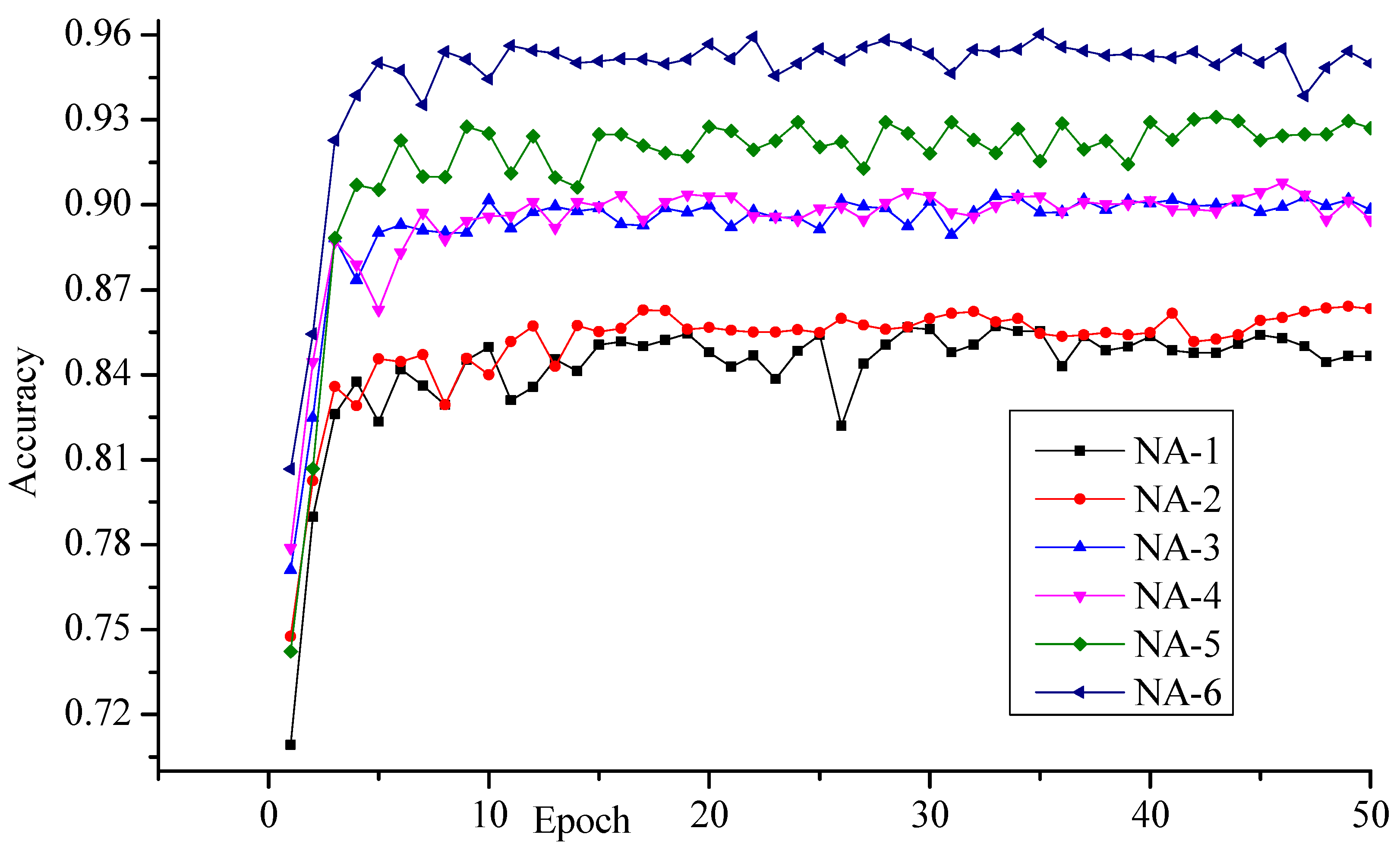
The best recognition accuracy was obtained with the network architecture NA-6, and the least recognition accuracy was obtained with the network architecture NA-1. Figure 3 shows the obtained recognition accuracy at each epoch. The network NA-1 produced 85% recognition accuracy because it has only one convolutional layer. The network NA-3 and NA-5 produced higher recognition accuracies of 91.53% and 93.24% respectively because these networks have a more convolutional layer. This enhancement signifies that the increment of the convolutional layer in deep convolutional neural network produced best results. In our experiments, we observed the enhancement in the recognition accuracy by increasing the number of kernels of convolutional layer. The network architectures NA-2, NA-4 and NA-6 had more kernels than NA-1, NA-3 and NA-5 and they produced higher recognition accuracy as observed in Table 2. The number of trainable parameters for each network architecture is shown in Table 3. The entire network architecture was also tested using the RMSProp optimizer, and the results have reported in Table 4. The NA-6 network produced 96.02% recognition accuracy with RMSProp while 95.58% with Adam. The behavior of NA-6 with RMSProp at each epoch can be seen in Figure 4.
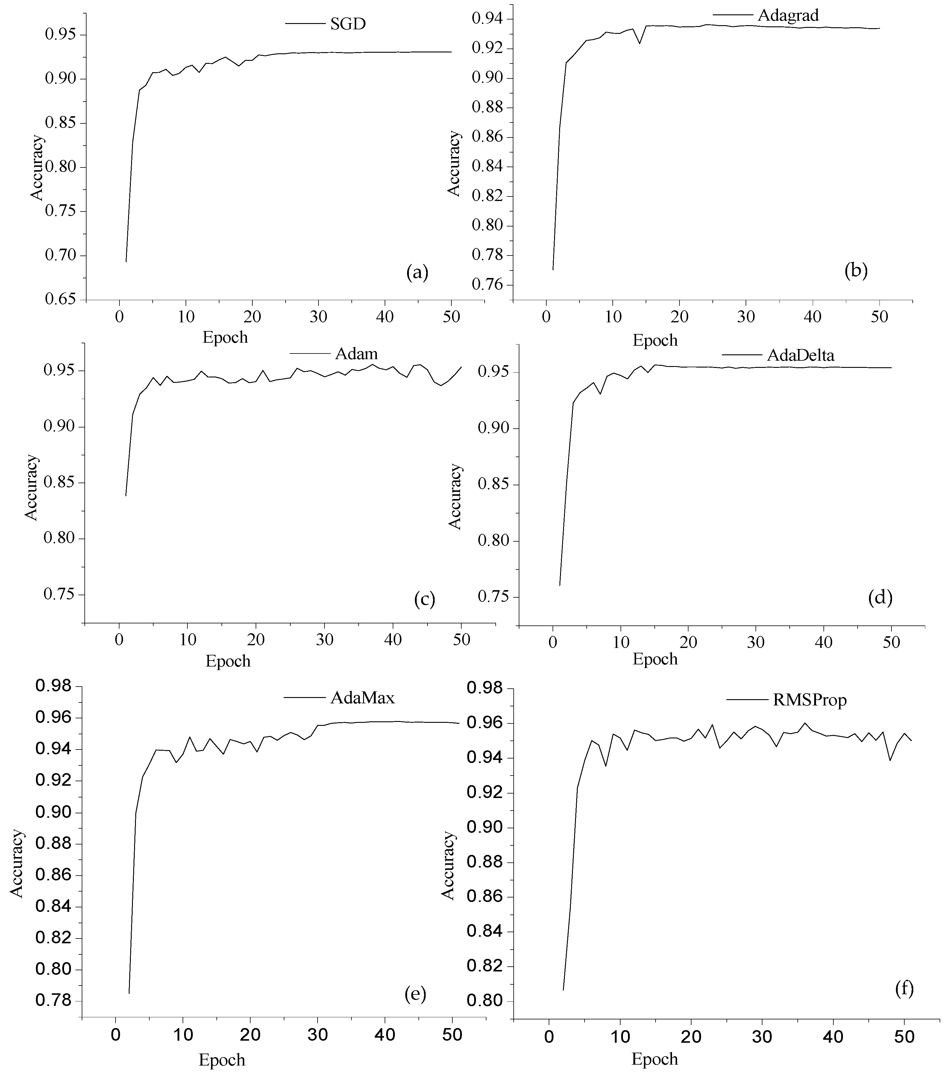
The best recognition accuracy of the ISIDCHAR database was obtained with NA-6 network architecture with RMSProp optimizer. However, it may be possible that this network could perform better with other optimizers. To further investigate, we performed experiments with six different optimizers. Table 5 shows the recognition accuracy obtained with NA-6 at different optimizers. The highest recognition accuracy 96.02% was recorded with NA-6 at RMSProp optimizer. The Adam optimizer outperformed the SGD and Adagrad optimizers. The AdaDelta, AdaMax, and RMSProp optimizers outperformed the Adam optimizer. Figure 5 shows the performance of individual optimizer.
We found that the NA-6 network architecture with RMSProp optimizer produced the highest recognition accuracy. This network was again trained by layer-wise model as described in Section 3.3.
This network was tested with ISIDCHAR, V2DMDCHAR, and combined databases. The results are reported in Table 6. It has been seen that a nice enhancement in the recognition accuracy was recorded by the layer-wise training model. The 97.30% recognition accuracy was obtained on ISIDCHAR database and 97.65% recognition accuracy obtained on V2DMDCHAR database. The layer-wise training model was also applied after combining both the databases and obtained 98% recognition accuracy when 70% of the samples were used for training and the rest used for testing. The current work is compared to previous works on ISIDCHAR database in Table 7.
5. Conclusions
Deep learning is one of the prominent technologies that have been experimentally studied with entire major areas of computer vision and document analysis. In this paper, we experimentally developed a deep convolutional neural network (DCNN) and adaptive gradient methods to recognize the unconstrained handwritten Devanagari characters. The deep convolutional neural network helped us to find the best features automatically and also classify them. We experimented with a handwritten Devanagari character database with six different DCNN network architectures as well as six different optimizers. The highest recognition accuracy 96.02% was obtained using NA-6 network architecture and RMSProp—an adaptive gradient method (optimizer). Further, we again trained DCNN layer-wise, which is also adopted by many researchers to enhance the recognition accuracy, using NA-6 network architecture and the RMSProp adaptive gradient method. Using DCNN layer-wise training model, our database obtained 98% recognition accuracy, which is the highest recognition accuracy of the database.
Acknowledgments
The authors are thankful to the ISI, Kolkata to provide a database and the Manipal University Jaipur to provide the supercomputing facility without this facility deep learning concept was not possible for the handwritten Devanagari characters.
Author Contributions
Mahesh Jangid has envisaged the study, designed the experiments, and wrote the manuscript. Sumit Srivastava performed some part of experiments and corrected the manuscript. Both authors read and approved the final manuscript.
Conflicts of Interest
The authors declare that they have no competing interests.
References
- Jürgen, S. Deep learning in neural networks: An overview. Neural Netw. 2015, 61, 85–117. [Google Scholar]
- Ciregan, D.; Meier, U.; Schmidhuber, J. Multi-column deep neural networks for image classification. In Proceedings of the IEEE Conference on Computer Vision and Pattern Recognition (CVPR), Providence, RI, USA, 16–21 June 2012. [Google Scholar]
- Krizhevsky, A.; Sutskever, I.; Hinton, G.E. Imagenet classification with deep convolutional neural networks. In Proceedings of the Advances in Neural Information Processing Systems, Lake Tahoe, NV, USA, 3–8 December 2012. [Google Scholar]
- Lecun, Y.; Bottou, L.; Bengio, Y.; Haffner, P. Gradient-based learning applied to document recognition. Proc. IEEE 1998, 86, 2278–2324. [Google Scholar] [CrossRef]
- Navneet, D.; Triggs, B. Histograms of oriented gradients for human detection. In Proceedings of the CVPR 2005 IEEE Computer Society Conference on Computer Vision and Pattern Recognition, San Diego, CA, USA, 20–25 June 2005; Volume 1. [Google Scholar]
- Lowe, D.G. Distinctive image features from scale-invariant keypoints. Int. J. Comput. Vis. 2004, 60, 91–110. [Google Scholar] [CrossRef]
- Surinta, O.; Karaaba, M.F.; Schomaker, L.R.B.; Wiering, M.A. Recognition of handwritten characters using local gradient feature descriptors. Eng. Appl. Artif. Intell. 2015, 45, 405–414. [Google Scholar] [CrossRef]
- Ojala, T.; Pietikäinen, M.; Harwood, D. A comparative study of texture measures with classification based on featured distributions. Pattern Recognit. 1996, 29, 51–59. [Google Scholar] [CrossRef]
- Bay, H.; Tuytelaars, T.; van Gool, L. Surf: Speeded up robust features. In Proceedings of the 9th European Conference on Computer Vision, Graz, Austria, 7–13 May 2006; pp. 404–417. [Google Scholar]
- Wang, X.; Paliwal, K.K. Feature extraction and dimensionality reduction algorithms and their applications in vowel recognition. Pattern Recognit. 2003, 36, 2429–2439. [Google Scholar] [CrossRef]
- Zeiler, M.D.; Rob, F. Visualizing and understanding convolutional networks. In Proceedings of the European Conference on Computer Vision, Zurich, Switzerland, 6–12 September 2014. [Google Scholar]
- Simonyan, K.; Andrew, Z. Very deep convolutional networks for large-scale image recognition. arXiv, 2004; arXiv:1409.1556. [Google Scholar]
- Jaderberg, M.; Simonyan, K.; Zisserman, A. Spatial transformer networks. In Proceedings of the Advances in Neural Information Processing Systems, Montreal, QC, Canada, 11–12 December 2015. [Google Scholar]
- Cireşan, D.; Ueli, M. Multi-column deep neural networks for offline handwritten Chinese character classification. In Proceedings of the 2015 International Joint Conference on Neural Networks (IJCNN), Killarney, Ireland, 12–17 July 2015. [Google Scholar]
- Sarkhel, R.; Das, N.; Das, A.; Kundu, M.; Nasipuri, M. A Multi-scale Deep Quad Tree Based Feature Extraction Method for the Recognition of Isolated Handwritten Characters of popular Indic Scripts. Pattern Recognit. 2017, 71, 78–93. [Google Scholar] [CrossRef]
- Ahranjany, S.S.; Razzazi, F.; Ghassemian, M.H. A very high accuracy handwritten character recognition system for Farsi/Arabic digits using Convolutional Neural Networks. In Proceedings of the 2010 IEEE Fifth International Conference on Bio-Inspired Computing: Theories and Applications (BIC-TA), Changsha, China, 23–26 September 2010. [Google Scholar]
- Sethi, I.K.; Chatterjee, B. Machine Recognition of Hand-printed Devnagri Numerals. IETE J. Res. 1976, 22, 532–535. [Google Scholar] [CrossRef]
- Sharma, N.; Pal, U.; Kimura, F.; Pal, S. Recognition of off-line handwritten devnagari characters using quadratic classifier. In Computer Vision, Graphics and Image Processing; Springer: Berlin/Heidelberg, Germany, 2006; pp. 805–816. [Google Scholar]
- Deshpande, P.S.; Malik, L.; Arora, S. Fine Classification & Recognition of Hand Written Devnagari Characters with Regular Expressions & Minimum Edit Distance Method. JCP 2008, 3, 11–17. [Google Scholar]
- Arora, S.; Bhatcharjee, D.; Nasipuri, M.; Malik, L. A two stage classification approach for handwritten Devnagari characters. In Proceedings of the International Conference on Computational Intelligence and Multimedia Applications, Sivakasi, Tamil Nadu, India, 13–15 December 2007; Volume 2, pp. 399–403. [Google Scholar]
- Arora, S.; Bhattacharjee, D.; Nasipuri, M.; Basu, D.K.; Kundu, M.; Malik, L. Study of different features on handwritten Devnagari character. In Proceedings of the 2009 2nd International Conference on Emerging Trends in Engineering and Technology (ICETET), Nagpur, India, 16–18 December 2009; pp. 929–933. [Google Scholar]
- Hanmandlu, M.; Murthy, O.V.R.; Madasu, V.K. Fuzzy Model based recognition of handwritten Hindi characters. In Proceedings of the 9th Biennial Conference of the Australian Pattern Recognition Society on Digital Image Computing Techniques and Applications, Glenelg, Australia, 3–5 December 2007; pp. 454–461. [Google Scholar]
- Arora, S.; Bhattacharjee, D.; Nasipuri, M.; Basu, D.K.; Kundu, M. Recognition of non-compound handwritten devnagari characters using a combination of mlp and minimum edit distance. arXiv, 2010; arXiv:1006.5908. [Google Scholar]
- Kumar, S. Performance comparison of features on Devanagari handprinted dataset. Int. J. Recent Trends 2009, 1, 33–37. [Google Scholar]
- Pal, U.; Sharma, N.; Wakabayashi, T.; Kimura, F. Off-line handwritten character recognition of devnagari script. In Proceedings of the Ninth International Conference on Document Analysis and Recognition, Curitiba, Parana, Brazil, 23–26 September 2007; Volume 1, pp. 496–500. [Google Scholar]
- Pal, U.; Wakabayashi, T.; Kimura, F. Comparative study of Devnagari handwritten character recognition using different feature and classifiers. In Proceedings of the 10th International Conference on Document Analysis and Recognition, Catalonia, Spain, 26–29 July 2009; pp. 1111–1115. [Google Scholar]
- Duchi, J.; Hazan, E.; Singer, Y. Adaptive subgradient methods for online learning and stochastic optimization. J. Mach. Learn. Res. 2011, 12, 2121–2159. [Google Scholar]
- Zeiler, M.D. ADADELTA: an adaptive learning rate method. arXiv, 2012; arXiv:1212.5701. [Google Scholar]
- Hinton, G. Slide 6, Lecture Slide 6 of Geoffrey Hinton’s Course. Available online: http://www.cs.toronto.edu/∼tijmen/csc321/slides/lecture_slides_lec6.pdf (accessed on 19 July 2017).
- Kingma, D.; Jimmy, B. Adam: A method for stochastic optimization. arXiv, 2014; arXiv:1412.6980. [Google Scholar]
- Dongre, V.J.; Vijay, H.M. Devnagari handwritten numeral recognition using geometric features and statistical combination classifier. arXiv, 2013; arXiv:1310.5619. [Google Scholar]
- Jangid, M.; Sumit, S. Gradient local auto-correlation for handwritten Devanagari character recognition. In Proceedings of the 2014 International Conference on High Performance Computing and Applications (ICHPCA), Bhubaneswar, India, 22–24 December 2014. [Google Scholar]
- Jangid, M.; Sumit, S. Similar handwritten Devanagari character recognition by critical region estimation. In Proceedings of the 2016 International Conference on Advances in Computing, Communications and Informatics (ICACCI), Jaipur, India, 21–24 September 2016. [Google Scholar]
Figure 1.
The schematic diagram of deep convolutional neural network (DCNN) architecture.
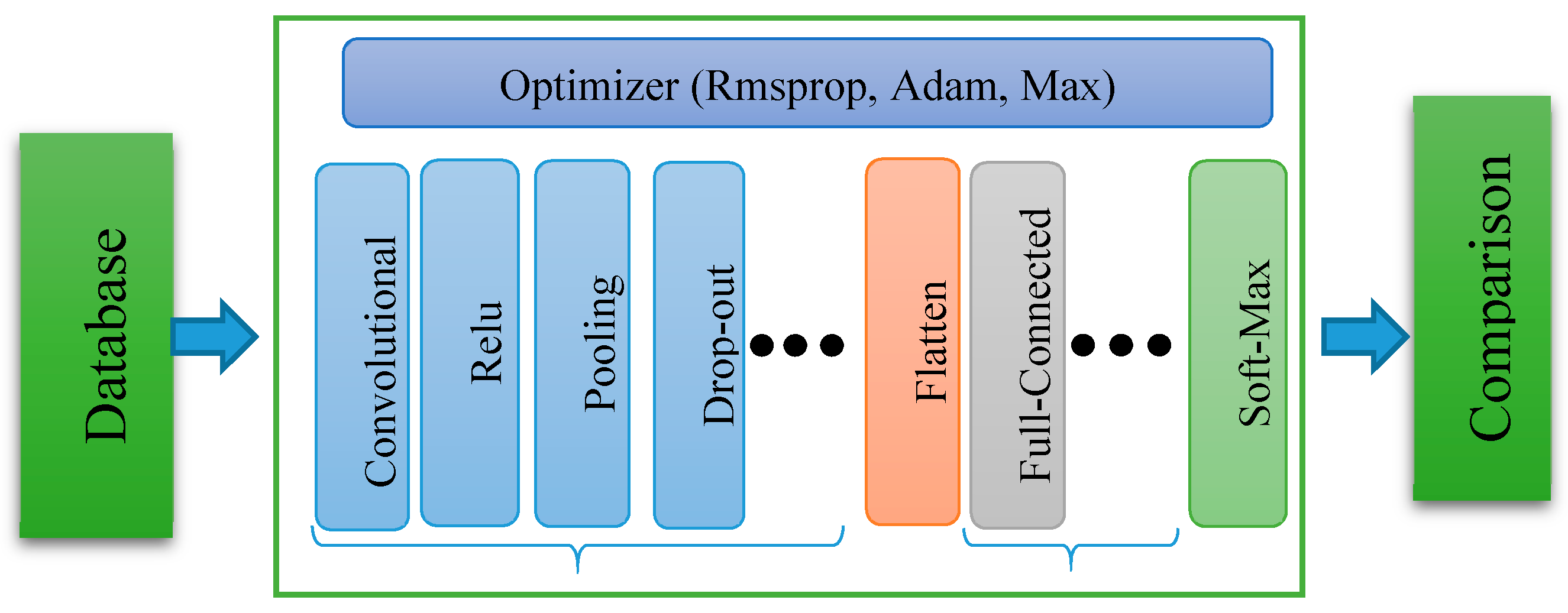
Figure 2.
Layer-wise training of deep convolutional neural network.
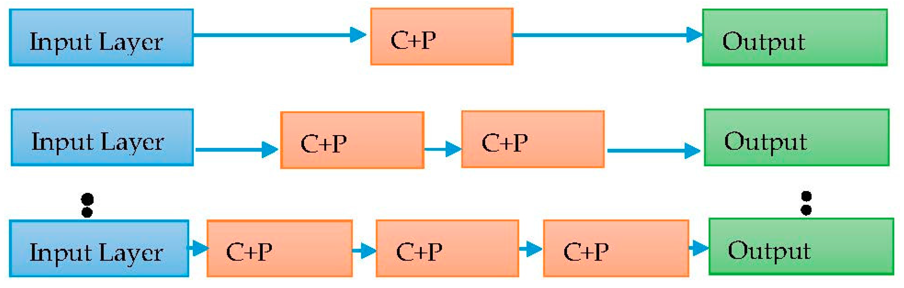
Figure 3.
In this figure, we draw the recognition accuracy obtained with different network architectures on ISIDCHAR database at each epoch. The Adam optimizer was used.
Figure 3.
In this figure, we draw the recognition accuracy obtained with different network architectures on ISIDCHAR database at each epoch. The Adam optimizer was used.
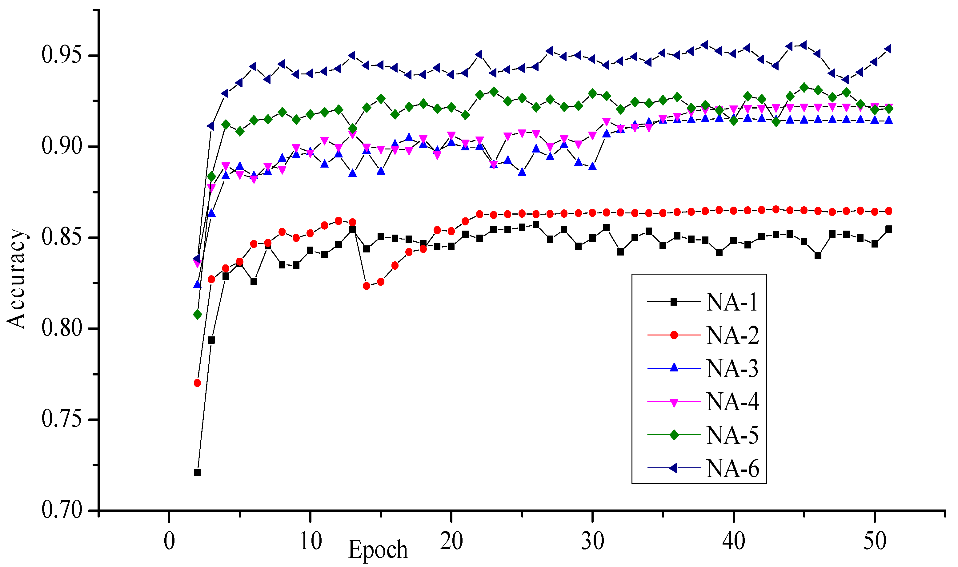
Figure 4.
In this figure, we draw the recognition accuracy obtained with different network architectures on the ISIDCHAR database at each epoch. The RMSProp optimizer was used.
Figure 4.
In this figure, we draw the recognition accuracy obtained with different network architectures on the ISIDCHAR database at each epoch. The RMSProp optimizer was used.

Figure 5.
In this figure, we draw the recognition accuracy obtained with NA-6 network architecture at different optimizers (a) SGD; (b) Adagrad; (c) Adam; (d) AdaDelta; (e) AdaMax; (f) RMSProp; on the ISIDCHAR database at each epoch.
Figure 5.
In this figure, we draw the recognition accuracy obtained with NA-6 network architecture at different optimizers (a) SGD; (b) Adagrad; (c) Adam; (d) AdaDelta; (e) AdaMax; (f) RMSProp; on the ISIDCHAR database at each epoch.

Table 1.
Various network architectures of deep convolutional neural network used.
| Network | Model Architectures |
|---|---|
| NA-1 | 64IN64-64C2-Relu-4P2-500FC-47OU |
| NA-2 | 64IN64-64C2-Relu-4P2-1000FC-47OU |
| NA-3 | 64IN64-32C2-Relu-4P2-32C2-Relu-4P2-1000FC-47OU |
| NA-4 | 64IN64-64C2-Relu-4P2-64C2-Relu-4P2-1000FC-47OU |
| NA-5 | 64IN64-32C2-Relu-4P2-32C2-Relu-4P2-32C2-Relu-4P2-1000FC-47OU |
| NA-6 | 64IN64-64C2-Relu-4P2-64C2-Relu-4P2-64C2-Relu-4P2-1000FC-47OU |
Table 2.
In this table, we report the results in term of maximum, minimum, mean, and standard deviation recognition accuracy obtained with different network architectures on ISIDCHAR when the system trained for 50 epochs with the Adam optimizer. The best scores are in bold.
Table 2.
In this table, we report the results in term of maximum, minimum, mean, and standard deviation recognition accuracy obtained with different network architectures on ISIDCHAR when the system trained for 50 epochs with the Adam optimizer. The best scores are in bold.
| Recognition Accuracy | Different Network Architectures | |||||
|---|---|---|---|---|---|---|
| NA-1 | NA-2 | NA-3 | NA-4 | NA-5 | NA-6 | |
| Maximum | 0.8571 | 0.8654 | 0.9153 | 0.9224 | 0.9324 | 0.9558 |
| Minimum | 0.7208 | 0.7701 | 0.8237 | 0.8363 | 0.8077 | 0.8385 |
| Average | 0.8436 | 0.8549 | 0.9000 | 0.9058 | 0.9190 | 0.9427 |
| Std. Deviation | 0.0204 | 0.0169 | 0.0165 | 0.0158 | 0.0178 | 0.0168 |
Table 3.
List of trainable parameters in each network architecture.
| Network Architectures | Layer Type | Layer Size | Trainable Parameters | Total Parameters |
|---|---|---|---|---|
| NA-1 | Conv1 layer | 64 × 64 × 64 | 1088 | 34,873,135 |
| Dense layer | 500 | 34,848,500 | ||
| Output layer | 47 | 23,547 | ||
| NA-2 | Conv1 layer | 64 × 64 × 64 | 1088 | 61,553,135 |
| Dense layer | 1000 | 61,505,000 | ||
| Output layer | 47 | 47,047 | ||
| NA-3 | Conv1 layer | 32 × 64 × 64 | 544 | 7,265,007 |
| Conv2 layer | 32 × 33 × 33 | 16,416 | ||
| Dense layer | 1000 | 7,201,000 | ||
| Output layer | 47 | 47,047 | ||
| NA-4 | Conv1 layer | 64 × 64 × 64 | 1088 | 14,514,735 |
| Conv2 layer | 64 × 33 × 33 | 65,600 | ||
| Dense layer | 1000 | 14,401,000 | ||
| Output layer | 47 | 47,047 | ||
| NA-5 | Conv1 layer | 32 × 64 × 64 | 544 | 1,649,423 |
| Conv2 layer | 32 × 33 × 33 | 16,416 | ||
| Conv3 layer | 32 × 17 × 17 | 16,416 | ||
| Dense layer | 1000 | 1,569,000 | ||
| Output layer | 47 | 47,047 | ||
| NA-6 | Conv1 layer | 64 × 64 × 64 | 1088 | 3,316,335 |
| Conv2 layer | 64 × 33 × 33 | 65,600 | ||
| Conv3 layer | 64 × 17 × 17 | 65,600 | ||
| Dense layer | 1000 | 3,137,000 | ||
| Output layer | 47 | 47,047 |
Table 4.
In this table, we report the results in term of maximum, minimum, mean, and standard deviation recognition accuracy obtained with different network architectures on ISIDCHAR when the system trained for 50 epochs with the RMSProp optimizer. The best scores are in bold.
Table 4.
In this table, we report the results in term of maximum, minimum, mean, and standard deviation recognition accuracy obtained with different network architectures on ISIDCHAR when the system trained for 50 epochs with the RMSProp optimizer. The best scores are in bold.
| Recognition Accuracy | Different Network Architectures | |||||
|---|---|---|---|---|---|---|
| NA-1 | NA-2 | NA-3 | NA-4 | NA-5 | NA-6 | |
| Maximum | 0.8572 | 0.8641 | 0.903 | 0.9079 | 0.9311 | 0.9602 |
| Minimum | 0.7093 | 0.7475 | 0.7711 | 0.7788 | 0.7422 | 0.8067 |
| Average | 0.8383 | 0.8501 | 0.8927 | 0.8941 | 0.9150 | 0.9463 |
| Std. Deviation | 0.0321 | 0.0232 | 0.0210 | 0.0197 | 0.0308 | 0.0252 |
Table 5.
In this table, we report the results in term of maximum, minimum, mean, and standard deviation recognition accuracy obtained with NA-6 on ISIDCHAR when the system trained for 50 epochs with the different optimizers. The best scores are in bold.
Table 5.
In this table, we report the results in term of maximum, minimum, mean, and standard deviation recognition accuracy obtained with NA-6 on ISIDCHAR when the system trained for 50 epochs with the different optimizers. The best scores are in bold.
| Recognition Accuracy | Different Optimizers | |||||
|---|---|---|---|---|---|---|
| SGD | Adagrad | Adam | AdaDelta | AdaMax | RMSProp | |
| Maximum | 0.931 | 0.9364 | 0.9558 | 0.9565 | 0.9579 | 0.9602 |
| Minimum | 0.6933 | 0.7703 | 0.7585 | 0.7605 | 0.7851 | 0.8067 |
| Mean | 0.9168 | 0.9280 | 0.9411 | 0.9457 | 0.9448 | 0.9463 |
| Std. Deviation | 0.0365 | 0.0252 | 0.0274 | 0.0311 | 0.0256 | 0.0252 |
Table 6.
In this table, we reported the maximum recognition accuracy obtained with NA-6 and RMSProp optimizer on ISIDCHAR, V2DMDCHAR and combined both when the model was trained layer-wise.
Table 6.
In this table, we reported the maximum recognition accuracy obtained with NA-6 and RMSProp optimizer on ISIDCHAR, V2DMDCHAR and combined both when the model was trained layer-wise.
| Database | No. of Samples | Recognition Accuracy | |
|---|---|---|---|
| DCNN | Layer-Wise DCNN | ||
| ISIDCHAR | 36,172 | 96.02% | 97.30% |
| V2DMDCHAR | 20,305 | 96.45% | 97.65% |
| ISIDCHAR+V2DMDCHAR | 56,477 | 96.53% | 98.00% |
Table 7.
Comparison of recognition accuracy by other researchers.
| S. No. | Accuracy Obtained | Feature; Classifier | Method Proposed by | Data Size |
|---|---|---|---|---|
| 1 | 95.19 | Gradient; MIL | U. Pal [26] | 36,172 |
| 2 | 95.24 | GLAC; SVM | M. Jangid [32] | 36,172 |
| 3 | 96.58 | Masking, SVM | M. Jangid [33] | 36,172 |
| 4 | 96.45 | DCNN | Proposed work | 36,172 |
| 5 | 97.65 | SL-DCNN | Proposed work | 36,172 |
| 6 | 98 | SL-DCNN | Proposed work | 56,477 |
© 2018 by the authors. Licensee MDPI, Basel, Switzerland. This article is an open access article distributed under the terms and conditions of the Creative Commons Attribution (CC BY) license (http://creativecommons.org/licenses/by/4.0/).
Share and Cite
MDPI and ACS Style
Jangid, M.; Srivastava, S. Handwritten Devanagari Character Recognition Using Layer-Wise Training of Deep Convolutional Neural Networks and Adaptive Gradient Methods. J. Imaging 2018, 4, 41. https://doi.org/10.3390/jimaging4020041
AMA Style
Jangid M, Srivastava S. Handwritten Devanagari Character Recognition Using Layer-Wise Training of Deep Convolutional Neural Networks and Adaptive Gradient Methods. Journal of Imaging. 2018; 4(2):41. https://doi.org/10.3390/jimaging4020041
Chicago/Turabian StyleJangid, Mahesh, and Sumit Srivastava. 2018. "Handwritten Devanagari Character Recognition Using Layer-Wise Training of Deep Convolutional Neural Networks and Adaptive Gradient Methods" Journal of Imaging 4, no. 2: 41. https://doi.org/10.3390/jimaging4020041
Note that from the first issue of 2016, this journal uses article numbers instead of page numbers. See further details here.