Efficient Implementation of Gaussian and Laplacian Kernels for Feature Extraction from IP Fisheye Cameras

Abstract

The Gaussian kernel, its partial derivatives and the Laplacian kernel, applied at different image scales, play a very important role in image processing and in feature extraction from images. Although they have been extensively studied in the case of images acquired by projective cameras, this is not the case for cameras with fisheye lenses. This type of cameras is becoming very popular, since it exhibits a Field of View of 180 degrees. The model of fisheye image formation differs substantially from the simple projective transformation, causing straight lines to be imaged as curves. Thus the traditional kernels used for processing images acquired by projective cameras, are not optimal for fisheye images. This work uses the calibration of the acquiring fisheye camera to define a geodesic metric for distance between pixels in fisheye images and subsequently redefines the Gaussian kernel, its partial derivatives, as well as the Laplacian kernel. Finally, algorithms for applying in the spatial domain these kernels, as well as the Harris corner detector, are proposed, using efficient computational implementations. Comparative results are shown, in terms of correctness of image processing, efficiency of application for multi scale processing, as well as salient point extraction. Thus we conclude that the proposed algorithms allow the efficient application of standard processing and analysis techniques of fisheye images, in the spatial domain, once the calibration of the specific camera is available.

1. Introduction

A number of types of very wide field cameras acquire images with 180° field of view (FoV). These cameras use dioptric systems, spherical lens, often called fisheye, or a combination of catadioptric (parabolic or spherical mirror) and dioptric (normal projection lens), often referred to as omnidirectional. The model of formation of all these types of images differs significantly from the traditional central projection model and introduces rapid deterioration of spatial resolution towards the periphery of the FoV, as well as strong deformations that map straight lines as curves. The model of image formation with 180° FoV can be treated in a unified mathematic way, utilizing a spherical optic lens and central projection [1,2]. Thus we will use the terms interchangeably for the rest of the paper.

The use of very wide field cameras is becoming very wide in domains like security [3], robotics [4,5], public and private area monitoring, since they allow constant imaging of all directions with a single camera.

Spherical fisheye panoramas are used to emulate or to register a PTZ camera and to integrating live webcam feeds within 2D and 3D GIS applications (such as Google Earth and Google Maps) [6,7]. Fisheye cameras with special processing operators are proposed for large space monitoring and crowd counting in [8]. In [9], a network of fisheye cameras is used to efficiently track persons in a space with obstacles that hinder visibility. Traffic management at road intersection has been proposed in [10] using network fisheye cameras. Pair of fisheye cameras has been used for pose estimation and motion capture in [11], employing a number of 3D Gaussians to generate a probabilistic body model. Gaussian kernels defined in 3D have also been used for scene modeling, in order to make discrete phenomena, like occlusion, continuous and thus, more easily optimizable [12].

The very different model of image formation for fisheye images has invoked a number of attempts to redefine image processing operators for this type of images. The basic morphology operators have been redefined in [8], although the computational cost has not been discussed.

The well-known Scale-Invariant Feature Transform (SIFT) image descriptors that were introduced in [13], are redefined for omnidirectional images in [14] in the frequency domain. Fisheye images are defined over spherical coordinates (azimuth θ, elevation φ). Therefore, Spherical Fourier Transform (SFT) is used, that decomposes the image as a weighted sum of spherical harmonic functions $Y_l^m\left(\mathsf{\theta },\mathsf{\phi }\right)$ of degree l and order m, with $\left|m\right|\le l$. In [15], the Gaussian kernel has been defined in the (θ, φ) image domain using spherical harmonics of the 0th order. The work of [16] also employs the use of SFT to detect points of interest using the well-known SIFT. In [17] differential operators defined on Riemannian manifolds are used to compute scale space and perform smoothing in fisheye images. That work was furthr improved in [18], where the already developed differential operator was extended to perform SHIFT-like salient point detection in omnidirectional images.

Others have reported exploiting the image space, rather than the frequency domain, for specific kernels. In [19], the authors also used a simplified version of SIFT feature extraction method (e.g., no multiresolution was used) for robot navigation by fisheye camera, obtaining good results. In [20], features are extracted from 360 FoV omnidirectional images in the spatial domain, but after the image has been mapped to a hexagonal grid. In [21], 4-neighbours and 8-neighbours Laplacian operators have been proposed for omnidirectional panoramic images. In [22], an approach for fisheye image processing in the spatial domain is proposed, using geodesic distance between pixels.

The approach proposed in this work, is also based on the spatial image domain and utilizes the geodesic distance between pixels. The main difference from [22] is that the proposed method uses the geodesic distance metric between pixels to redefine the basic filter kernels, whereas in [22] the image neighborhood is being resampled, while keeping the filter kernels unchanged. In order to avoid computationally expensive image interpolation, [22] uses the nearest neighbor interpolation, which although not a good performing technique, still produced better results than the classic image processing operators. As it will be discussed later, there is no proposed efficient implementation for the method in [22], since it requires the geodesic neighborhood definition for every pixel in each new image, in contrast to the method proposed in this work that requires the construction of a small Gaussian kernel, only once for a calibrated camera.

The rest of the paper is structured as following: In the methodology section, the geodesic distance metric is defined using the calibration of the fisheye camera. The Gaussian kernel, its partial derivatives and the Laplacian of Gaussian kernel is redefined, using the geodesic distance. All these kernels vary with their spatial location in the image, therefor, their direct convolution with the image is inefficient. Thus, an efficient computational implementation is proposed, which involves the initial pre-calculation of a single Gaussian kernel with small standard deviation σ₀ and the approximation of the Image response of the Gaussian, its derivatives, as well as the Laplacian of Gaussian at larger values of σ.

2. Materials and Methods

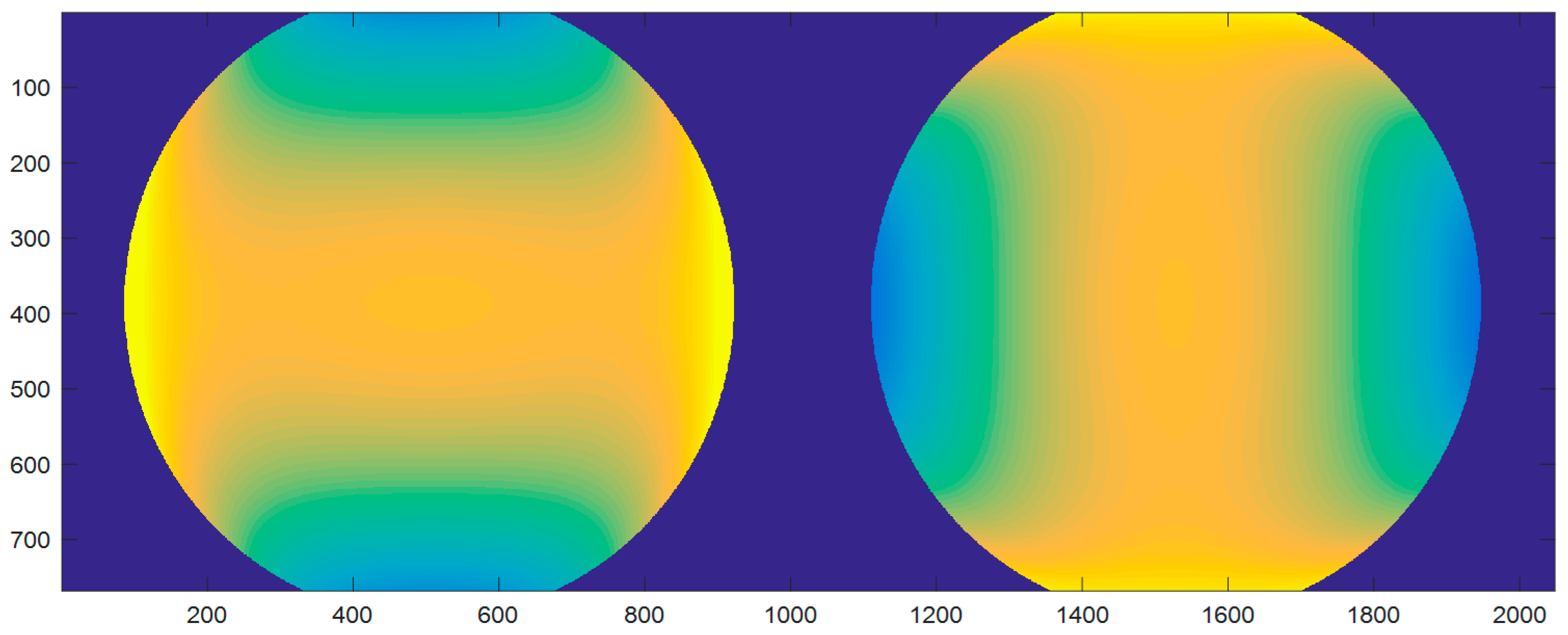
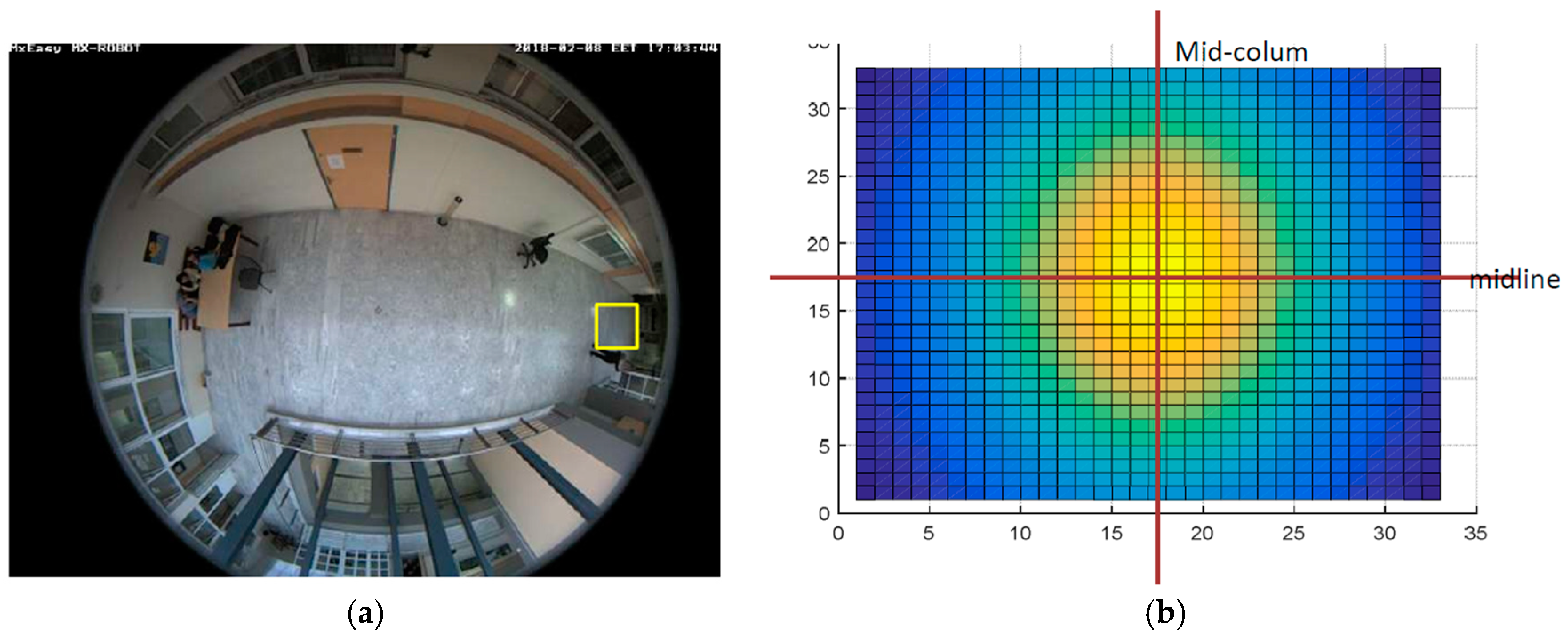
The methodology that is proposed in this work is tested with images acquired by a Mobotix Q24 fisheye camera, that is installed on the roof, imaging an indoor space. A typical frame of the camera is shown in Figure 1, with pixilation of 480 × 640. The camera has been calibrated using [23]. The result of the calibration is shown in Figure 2, where the azimuthal angle Θ and the elevation Φ is provided for each pixel of the fisheye image.

2.1. Geodesic Distance Metric between Pixels of the Calibrated Fish-Eye Image

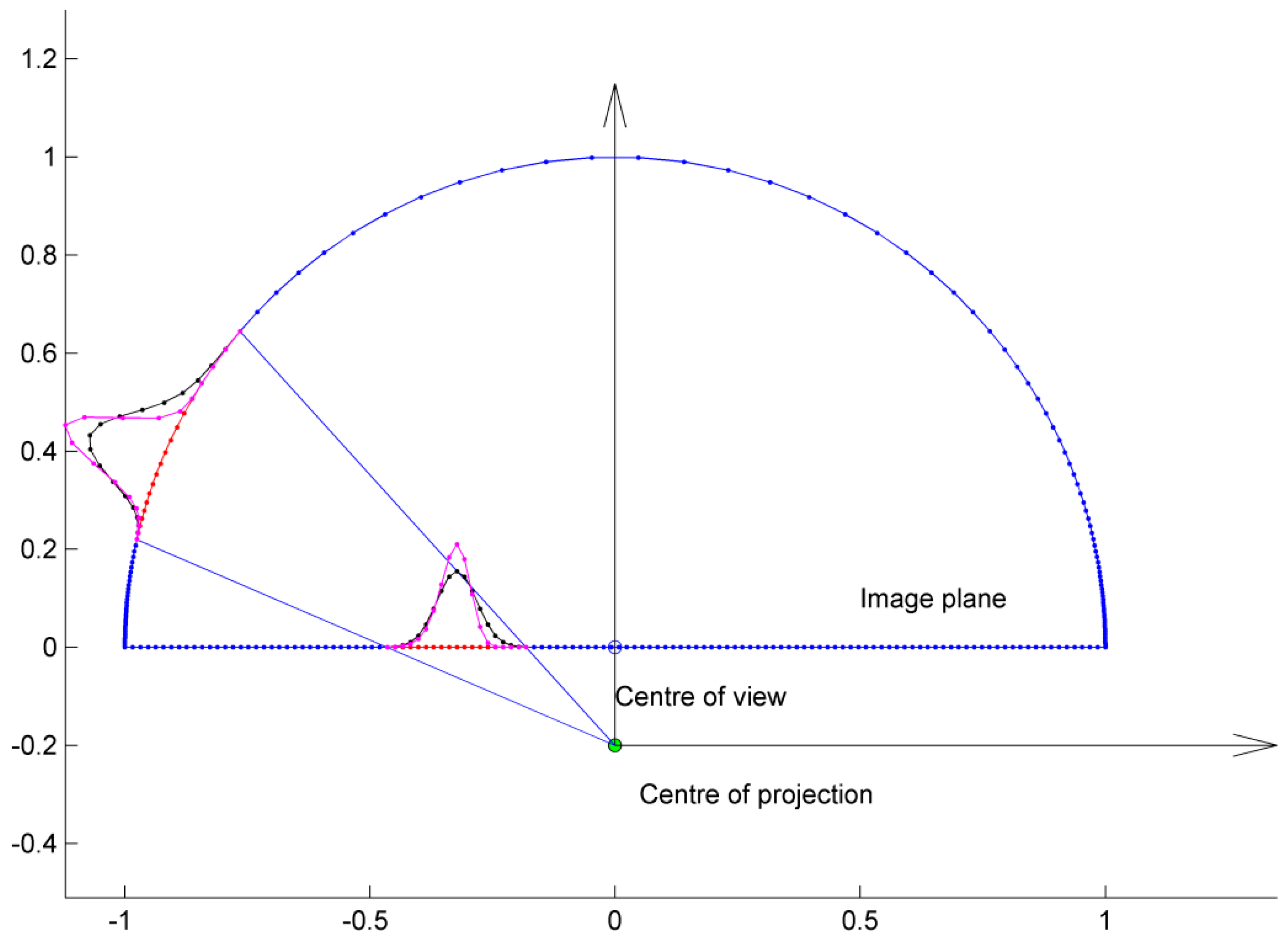
The formation of omni-directional image using a spherical lens, as presented in detail in [23] can be summarized as following: the intersection of the line connecting the real world point with the center of the optical element is calculated with the optical element. This intersection is then projected centrally on the image sensor plane. It has been shown [1] that by choosing the center of projection, one can simulate the use of any quadratic shape mirror (spherical, ellipsoid, paraboloid and hyperboloid). This type of image formation induces non-linear transformation of distances between pixels.

These concepts are visualized in Figure 3, where the semi-spherical optical element of unit radius and the image plane is displayed. The center of projection is placed at −f on the Y axis, with f set to 0.2. The image plane is tessellated into 128 equidistant points to resemble the image pixels. 21 of these “pixels” are backprojected on the spherical optical element (both shown in different color). It is self-evident that the back-projected points are no longer equidistant.

If a window of size (2w + 1, 1) is defined on the image plane (red dots in Figure 3, then the definition of a Gaussian within this window, using the Euclidean distance between pixels on the image plane is visualized as the black curve in Figure 3. If this Gaussian is back-projected on the spherical optical element, the kernel depicted in black (at the periphery) is produced. As expected, it is different from a Gaussian kernel, due to distance metric. In order to generate a Gaussian kernel defined on the image sensor, we have to modify the distance metric between pixels on the sensor, according to the geodesic distance of their back-projection on the circle. Figure 3 is a 2D abstraction of the real 3D camera setup. The asymmetry that is evident in the 21-point, black kernel, defined on the image plane is exaggerated since the image plane (image line in this 2D abstraction) was tessellated to only 128 pixels. Furthermore, in the case of a 2D kernel, asymmetry is present only along one of its two axes, as it will be further discussed below.

In [24] the use of the geodesic distance has been proposed for re-defining the Zernike moment invariant for calibrated fish-eye images. The proposed approach requires the results of the calibration of the fish-eye camera. Several approaches exist for fish-eye camera calibration, such as [1,25]. In this work, we utilize the calibration of the specific fish-eye camera, proposed in [23]. The results of the calibration nay be summarized in two look-up tables of size equal to an image frame, which hold the direction of each image pixel (x, y) in real 3D world. The direction is defined by two angles, the azimuth Θ(x, y) and the elevation Φ(x, y). During the calibration step, these two angles are pre-calculated for all pixels of the video frame and are stored in two look-up tables Θ and Φ, as shown in Figure 2.

It is clear that the distance of two pixels is different when measured on the image sensor and on the projection of the image points on the spherical optical element. Therefore, in order to produce accurate results, image processing algorithms that use pixel distances have to be re-implemented for fish-eye (omni-directional) images.

It is well known that the geodesic curve of a sphere is a great circle (a circle that lies on the sphere and has the same center with the sphere). Thus, the distance between any two points on a sphere is the length of the arc that is defined by the two points and belongs to a circle that passes through the two points and has the same centre with the sphere. The geodesic distance between pixels ${\mathit{p}}_0=\left(x_0,y_0\right)$ and ${\mathit{p}}_1=\left(x_1,y_1\right)$ is defined in [22,24] and can be summarized as following:

Let P₀ and P₁ be the projections of the two pixels on the spherical optical element and $v_0,v_1$ be the position vectors pointing to P₀ and P₁. The direction of the two pixels in real world is given by the pre-calculated look-up tables:

$$\begin{array}{l}\left({\mathsf{\theta }}_0,{\mathsf{\phi }}_0\right)=\left(\mathsf{\Theta }\left(x_0,y_0\right),\mathsf{\Phi }\left(x_0,y_0\right)\right)\\ \left({\mathsf{\theta }}_1,{\mathsf{\phi }}_1\right)=\left(\mathsf{\Theta }\left(x_1,y_1\right),\mathsf{\Phi }\left(x_1,y_1\right)\right)\end{array}$$

(1)

Thus, the position vectors are calculated:

$$v_i=\left(\cos {\mathsf{\theta }}_i\cos {\mathsf{\phi }}_i,\sin {\mathsf{\theta }}_i\cos {\mathsf{\phi }}_i,\sin {\mathsf{\phi }}_i\right),i=0,1$$

(2)

The distance r₀₁ of points P₀ and P₁ on the unit sphere is easily calculated as the arc-length between P₀ and P₁, assuming that cos⁻¹ returns the result in radians:

$$r_{01}=d\left(v_0,v_1\right)={\cos }^{-1}\left(v_0\cdot v_1\right)$$

(3)

Figure 4 shows the geodesic distance component between successive pixels along lines (left) and columns (right), defined more formally as:

$$\begin{array}{l}{D}_x\left(x,y\right)=d\left(\left(x+1,y\right),\left(x,y\right)\right)\\ D_y\left(x,y\right)=d\left(\left(x,y+1\right),\left(x,y\right)\right)\end{array}$$

(4)

2.2. Filter Kernels for Fish-Eye Image Processing Based on the Geodesic Distance Metric between Image Pixels

The most versatile filter in image processing is the Gaussian. According to its definition for 2D images, the Gaussian can be written as

$$g\left(x,y;\mathsf{\sigma }\right)=\frac{1}{2\pi {\mathsf{\sigma }}^2}{e}^{-\frac{r^2}{2{\mathsf{\sigma }}^2}}$$

(5)

with $r^2=x^2+y^2$ being the distance of pixel (x, y) from the centre of the kernel. The discrete Gaussian is defined (at least) in the following

$$\left(x,y\right)\in \left[-3\lceil \mathsf{\sigma }\rceil ,3\lceil \mathsf{\sigma }\rceil \right]\times \left[-3\lceil \mathsf{\sigma }\rceil ,3\lceil \mathsf{\sigma }\rceil \right]$$

(6)

where $\lceil x\rceil$ is the operator returning the closest integer larger than x, for x > 0. The standard deviation σ is defined by the user in pixels, which equivalently defines the size of the kernel, according to Equation (6).

The above “classical” definition of the Gaussian needs to be modified for calibrated fish-eye images. Let us suppose that we require the linear convolution of the Gaussian kernel with a fish-eye image, at pixel $p_0=\left(x_0,y_0\right)$. Let $A_{\mathsf{\sigma }}$ denote the subimage centered at $\left(x_0,y_0\right)$:

$$A_{\mathsf{\sigma }}=\left[x_0-3\lceil \mathsf{\sigma }\rceil ,x_0+3\lceil \mathsf{\sigma }\rceil \right]\times \left[y_0-3\lceil \mathsf{\sigma }\rceil ,y_0+3\lceil \mathsf{\sigma }\rceil \right]$$

(7)

In the case of a calibrated fish-eye image, the definition of Equation (4) is modified as following:

• It is straightforward to use the geodesic distance metric between $p_0$ and any pixel $p_i=\left(x_i,y_i\right)$ in A_σ, thus $r_i=d\left(p_i,p_0\right)$
• σ is initially defined by the user in pixels. However, since the geodesic distance between pixels is used in Equation (1), the value of σ (in pixels) cannot be used. This becomes clear if one considers that the Gaussian has to approach 0 within $A_{\mathsf{\sigma }}$. Since $A_{\mathsf{\sigma }}$ was defined as a window centered on the current pixel, spanning ±3 σ, we set σ equal to (1/3) of the maximum geodesic distance between the central pixel $p_0$ and any pixel in $A_{\mathsf{\sigma }}$:

  $$\mathsf{\sigma }=\frac{1}{3}\max \left(\left\{r_i=d\left(p_i,p_0\right),p_i\in A_{\mathsf{\sigma }}\right\}\right).$$

  (8)
• Then σ is replaced in Equation (5).
  Thus, for a Gaussian centered at $p_0=\left(x_0,y_0\right)$, the

  $$g\left(x,y;\mathsf{\sigma }\right)=g\left(p;\mathsf{\sigma }\right)=\frac{1}{2\pi {\mathsf{\sigma }}^2}{e}^{-\frac{d{\left(p,p_0\right)}^2}{2{\mathsf{\sigma }}^2}}$$

  (9)

It becomes obvious that the Gaussian kernel now depends on its location on the fish-eye image. In order to define the Gaussian kernel with a specific size for the whole fisheye image, the following Algorithm 1 is used:

Algorithm 1. Initialization of the Gaussian kernel with small standard deviation.

The size of the window kernel (2 w + 1) × (2 w + 1) is defined. The value of the standard deviation σ is calculated as following: The window A0 is placed near the edge of the FoV, where pixel distances are smaller than other locations with high elevation φ and σ0 is calculated according to Equation (8). This value of σ0 is used for each location in the fisheye image.

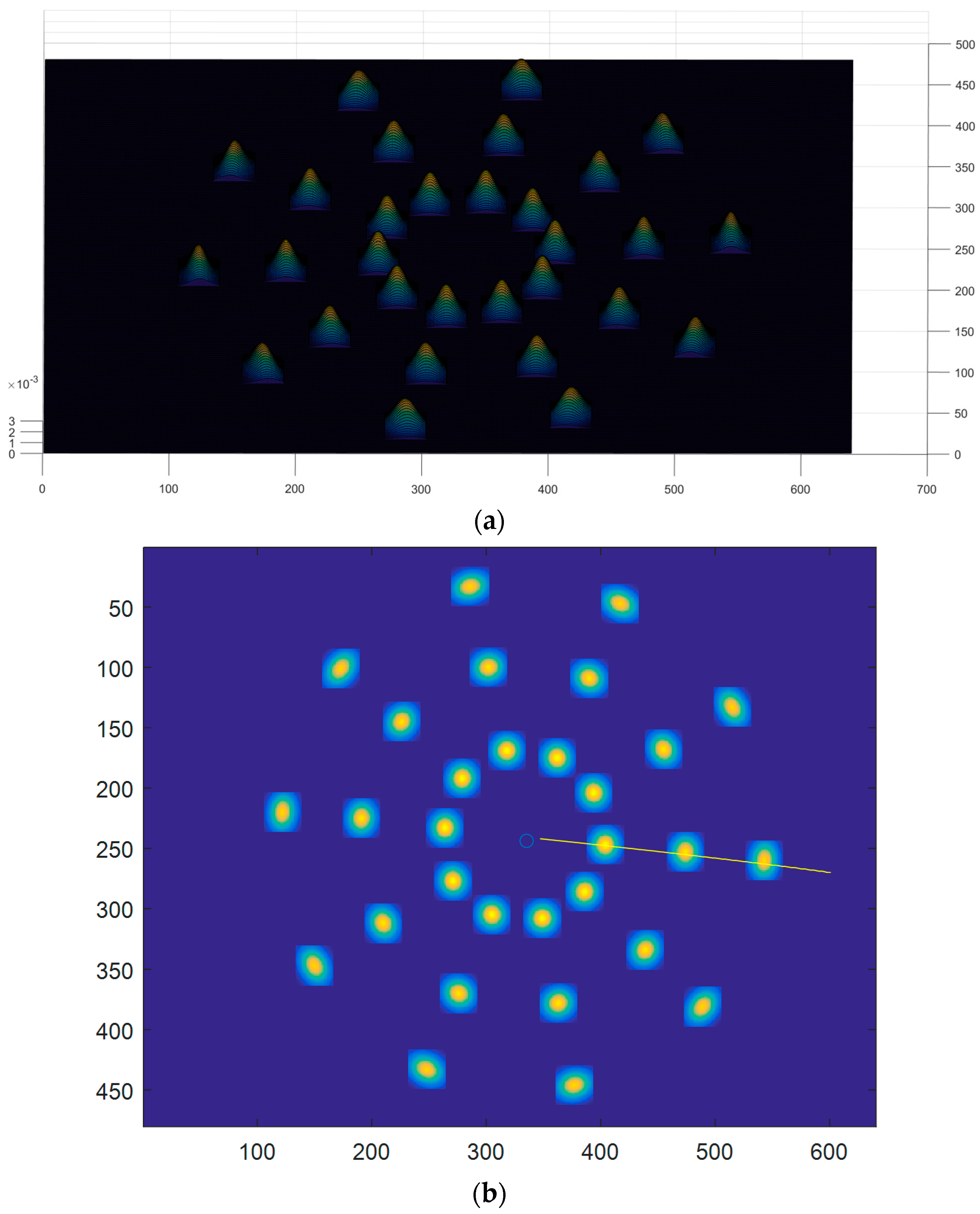
Figure 5a shows the Gaussian kernel as defined in Equation (9) at different position on the fisheye image. Radial lines emanating from the CoV (Center of View) have constant azimuthal θ and points on the concentric circles centered on the CoV have constant elevation φ. The same kernels are shown in (b), using color-scale. The CoV is marked on Figure 5b.

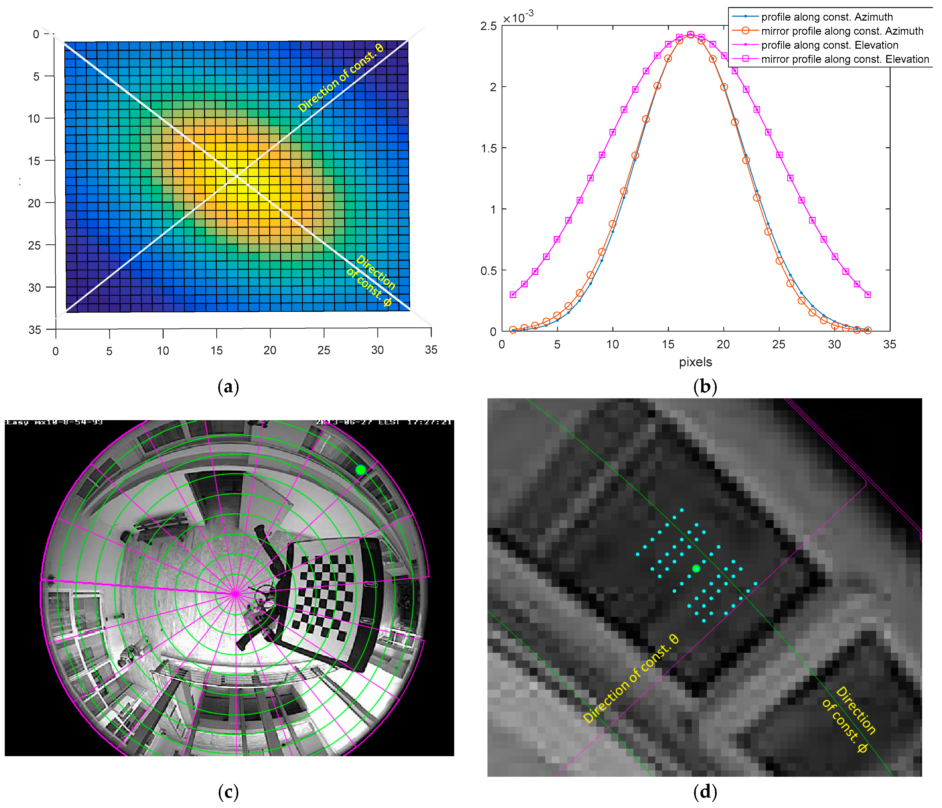
It is evident that the shape of the Gaussian kernel is a function of the kernel’s location on the image. More specifically, the kernel at pixel (x, y) appears rotated by an angle equal to the azimuth Θ(x, y) at this pixel. Furthermore, the Gaussian kernel exhibits asymmetry, as indicated in the 1D abstraction of Figure 3. It is easy to confirm that consecutive pixels along the direction with constant (iso-) elevation φ have constant geodesic distance. On the other hand, consecutive pixels along the direction with constant (iso-) azimuth θ do not have constant geodesic distance. Thus, the geodetic Gaussian kernel is expected to exhibit asymmetry along the axis with constant azimuth. An example depicting this asymmetry is shown in Figure 6. The location that was selected is shown in (c) as a green circle. The iso-azimuth and iso-elevation contours are superimposed in purple and green color respectively. Figure 6a shows a 35 × 35 geodetic Gaussian kernel, generated by Equation (9) of the proposed method. The orientation of the kernel with respect to the directions of constant azimuth and elevation, is as described above. Figure 6b displays the asymmetry of the kernel. More specifically, the profile of the kernel is plotted along the directions of constant azimuth θ and of constant elevation φ. Both profiles are also plotted after being mirrored, in order to make the asymmetry apparent. It can be observed that the kernel is symmetric along the direction of constant φ and slightly asymmetric along the direction of constant θ (the profile and its mirror do not match). Finally, the resampling of the image to construct the geodetic neighborhood round the selected point, as described in [22], Equation (16), is displayed in Figure 6d. These neighborhood pixels should be equidistant using geodesic distant metric and they were selected using the nearest neighbor interpolation, as explained in Section 3.3 of [22].

The partial derivatives of the Gaussian kernel are easily calculated analytically:

$$\frac{\partial }{\partial x}g\left(x,y;\mathsf{\sigma }\right)=g_x=-\frac{x}{{\mathsf{\sigma }}^2}g\left(x,y;\mathsf{\sigma }\right)$$

(10)

The x coordinate is calculated as the geodesic distance of (x, y) from (x₀, y), namely $x=d\left(\left(x_i,y_i\right),\left(x_0,y_i\right)\right)$. The same holds for the partial derivative with respect to y.

$$\begin{array}{l}\frac{\partial }{\partial x}g\left(x,y;\mathsf{\sigma }\right)=g_x=-\frac{d\left(\left(x,y\right),\left(x_0,y\right)\right)}{{\mathsf{\sigma }}^2}\frac{1}{2\pi {\mathsf{\sigma }}^2}{e}^{-\frac{d{\left(p,p_0\right)}^2}{2{\mathsf{\sigma }}^2}}\\ \frac{\partial }{\partial y}g\left(x,y;\mathsf{\sigma }\right)=g_y=-\frac{d\left(\left(x,y\right),\left(x,y_0\right)\right)}{{\mathsf{\sigma }}^2}\frac{1}{2\pi {\mathsf{\sigma }}^2}{e}^{-\frac{d{\left(p,p_0\right)}^2}{2{\mathsf{\sigma }}^2}}\end{array}$$

(11)

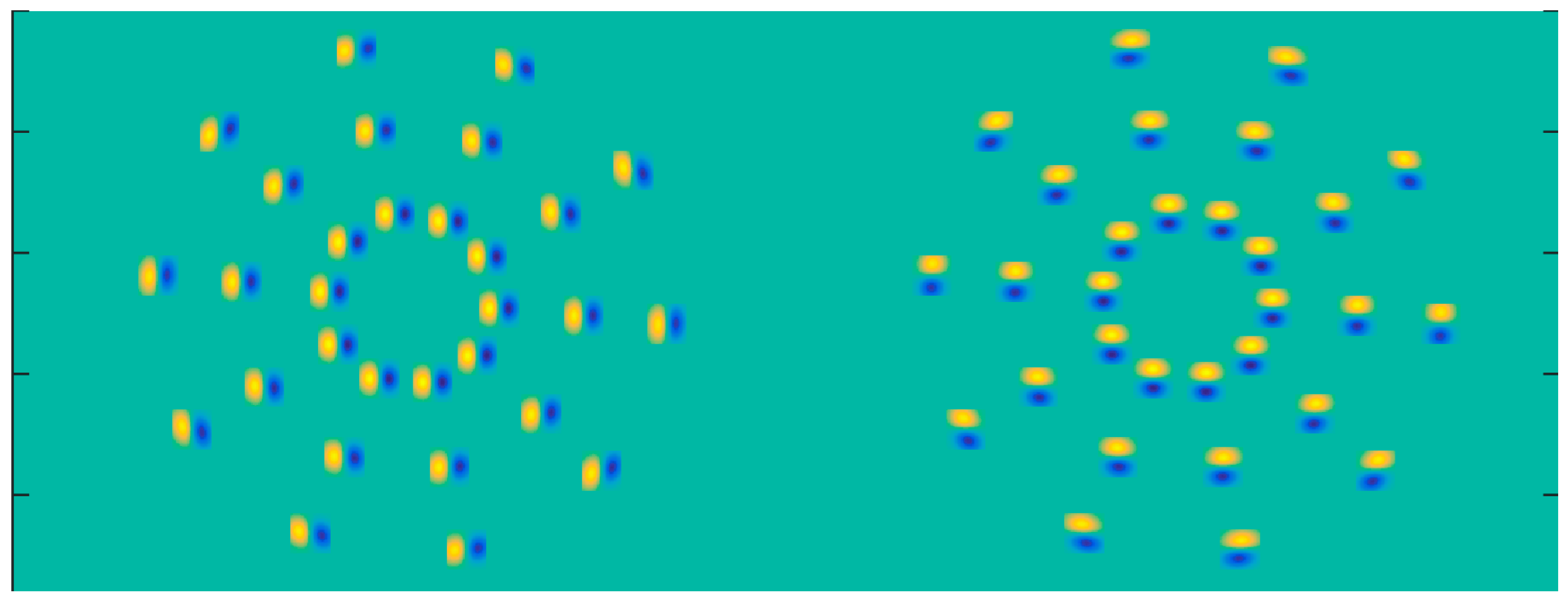
Figure 7 shows the two partial derivatives Gaussian kernel, as defined in Equation (11) at different position on the fisheye image. Radial lines emanating from the CoV have constant azimuthal θ. Points on the concentric circles centered on the CoV have constant elevation φ.

Similarly, the Laplacian of Gaussian for the calibrated fish-eye image is defined:

$$LoG\left(x,y;\mathsf{\sigma }\right)=\frac{d{\left(p,p_0\right)}^2-2{\mathsf{\sigma }}^2}{{\mathsf{\sigma }}^4}g\left(p;\mathsf{\sigma }\right)=\frac{d{\left(p,p_0\right)}^2-2{\mathsf{\sigma }}^2}{{\mathsf{\sigma }}^4}\frac{1}{2\pi {\mathsf{\sigma }}^2}{e}^{-\frac{d{\left(p,p_0\right)}^2}{2{\mathsf{\sigma }}^2}}$$

(12)

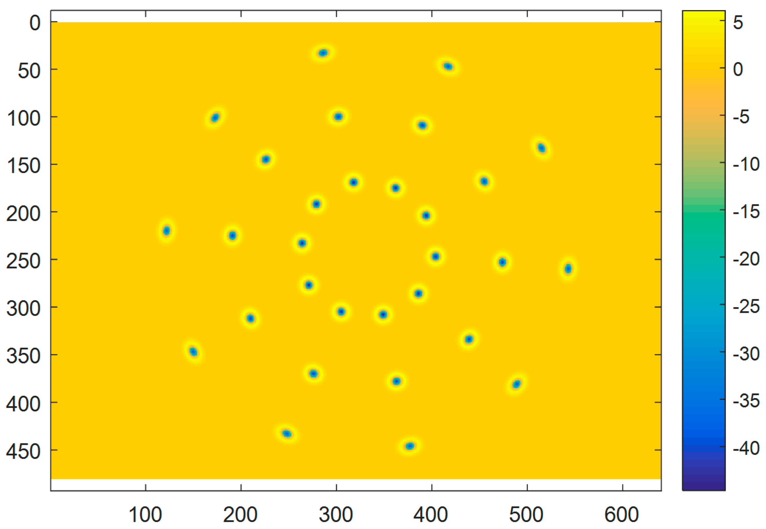
The LoG kernel is shown at different locations on the fisheye image in Figure 8. It can be easily observed that the LoG defined using the geodetic distance between pixels depends on the location of the pixel that it is applied to.

2.3. An Efficient Computational Implementation of the Geodetically Corrected g, g_x, g_y and LoG Kernels for Fisheye Images for Any Value of σ

The spatial dependence of the proposed geodetically corrected Gaussian kernel and its derivatives imposes a very high computational load, since the kernel itself has to be recomputed at each image pixel, prior to the actual convolution. In this section, an approach is presented that uses a small look-up table of the Gaussian kernel for a small pre-selected value of σ.

First we generate the Gaussian kernel for an image, using Equation (8), defined over a 5 × 5 image window. This is a demanding computation that only needs be performed once after the calibration of the camera. The Gaussian kernel is stored for each pixel of the fisheye image. Thus a total memory for a float array of N_L × N_c × 25 is required.

The method proposed in this work for the implementation of 2D convolution using Gaussian kernel with higher σ, is successive convolutions with a smaller, initially constructed Gaussian kernel. It is well known that convolving two Gaussians with standard deviations σ₁, σ₂ results in another Gaussian with σ² = σ₁² + σ₂². This fact is tested numerically in the case of the definition in Equation (9). More specifically, a point in the fisheye image is selected near the edge of the FoV where the deviation from the simple projective image formation is more significant. The initial Gaussian kernel g₀ is constructed according to Equation (9) with a stencil of 13 × 13. The standard deviation σ₀ of g₀ is calculated using Equation (8). A number of successive linear convolutions (*) is performed

g₀ * g₀ * g₀ * …* g₀

(13)

Thus, the result of the kth convolution should be a Gaussian with σ₀·(k + 1)^1/2.

Figure 9 shows the construction of a 33 × 33 stencil Gaussian kernel (b), at a position near the edge of FoV (a), using successive convolutions of an initial smaller 11 × 11 kernel (centered at the same pixel).

In order to facilitate visual comparison, the midline of each kernel is plotted as a curve in Figure 9d, up to the first 8 successive convolutions (the first kernel is the taller, narrower curve). The geodesic Gaussian that is generated using Equation (9) directly with the appropriate σ, is superimposed using symbol “□”. It can be observed that the result of the 8 successive convolutions with the small initial σ₀ is almost identical to the result of a single convolution with the much larger and computationally very demanding kernel. The asymmetry of the Gaussian kernel is shown in Figure 9c using the midline profile and the mid-column profile of the kernel, which in this specific location of the image, coincide with the direction of constant (iso-) azimuth and constant (iso-) elevation. The same two profiles are also plotted after reflection with respect to the middle point of the profiles. It can be observed that the mid-column profile is symmetric (the reflected profile matches the original profile), while the midline profile shows asymmetry (the profile and its reflection does not match). These findings are expected, according to the discussion in the previous subsection (Figure 6).

Thus, the proposed, efficient algorithm to calculate the convolution of a calibrated fisheye image I * g(x, y; σ) with a Gaussian with large values of standard deviation σ, using geodetic pixel distance, is as following Algorithm 2.

Algorithm 2. The proposed algorithm for calculating the response of a geodetically defined Gaussian kernel on a calibrated fisheye image, for large values of σ.

k = 0 Initialize g0 = g(x, y; σ0) while ${\mathsf{\sigma }}_0\sqrt{k+1}<{\mathsf{\sigma }}_g$   k = k + 1   I = I * g0 end

2.3.1. Approximating the Normalized Geodetic LoG Using DoG

The use of Difference of Gaussians (DoG) to approximate a Laplacian of Gaussian is well known in the literature [13], although the relation between the standard deviation of the two Gaussians and the Laplacian is seldom discussed in detail. Many approaches use the concept of octaves, namely define a number of convolution operations (typically 5) in order to double the value of σ and then resample the image to reduce the number of lines and column by two. The difference of the results of successive convolutions (DoG) approximates the convolution of the original image with the LoG. This multi-resolution approach is not directly applicable in the case of fisheye image processing, where generation of Gaussian kernels with different σ is computationally expensive. Thus the following approach is proposed, which consists of constructing a single geodetically corrected Gaussian kernel with small standard deviation ${\mathsf{\sigma }}_0$ (whose values depend on its spatial location on the image) and perform successive convolutions with this kernel. At the kth iteration, the standard deviation of the equivalent Gaussian kernel will be equal to

$$\mathsf{\sigma }={\mathsf{\sigma }}_0\sqrt{k+1}.$$

(14)

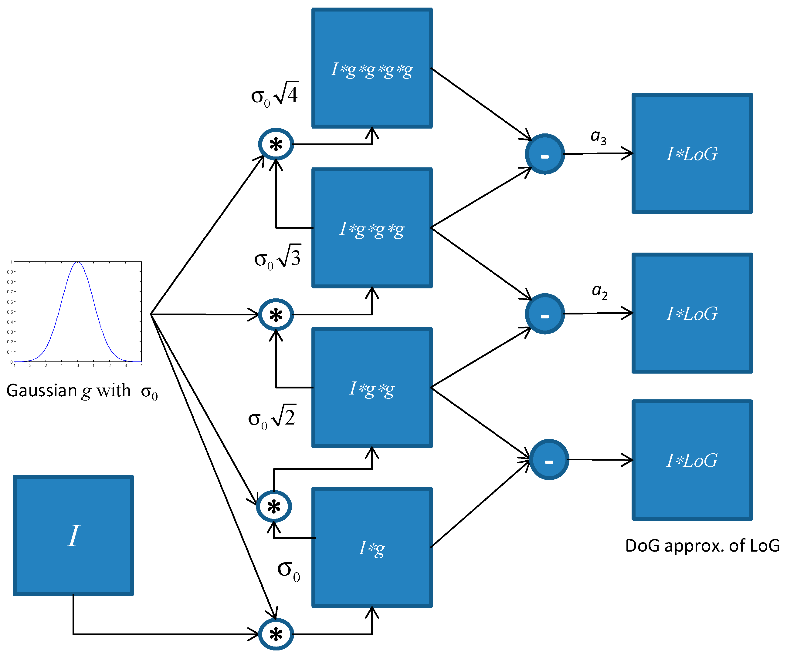
The iterations are stopped when the equivalent σ becomes greater than or equal to the required standard deviation. Differences of successive convolutions are assigned to I_L variable, since they approximate the response of the original image with the LoG. The factor a_k than normalizes the response of LoG with respect to σ is discussed. The steps of the Algorithm 3 for approximating the normalized LoG with DoG for a calibrated fisheye image are given below. A schematic diagram of the proposed algorithm is shown in Figure 10.

Algorithm 3. Approximating normalized LoG with DoG in the case of fisheye image.

k = 0 Initialize g0 = g(x, y; σ0), as in Equation (9) while ${\mathsf{\sigma }}_0\sqrt{k+1}<{\mathsf{\sigma }}_g$   k = k + 1   I1 = I * g0   IL = (I1 − I)ak   I = I1 end

Since LoG is used in the concept of different image scales, the response of the LoG needs to be normalized with respect to scale σ. It is well known that σ²·LoG is scale-normalized:

$${\mathsf{\sigma }}_2^2{\displaystyle \sum _x\left|LoG\left(x;{\mathsf{\sigma }}_2\right)\right|}={\displaystyle \sum _x{\mathsf{\sigma }}_1^2\left|LoG\left(x;{\mathsf{\sigma }}_1\right)\right|},{\mathsf{\sigma }}_2>{\mathsf{\sigma }}_1$$

(15)

It is easy to confirm that the partial derivative of a Gaussian with respect to σ is

$$\frac{\partial g\left(x;\mathsf{\sigma }\right)}{\partial \mathsf{\sigma }}=\mathsf{\sigma }\cdot LoG$$

If the derivative is approximated using finite differences, then

$$\frac{\partial g\left(x;\mathsf{\sigma }\right)}{\partial \mathsf{\sigma }}=\frac{g\left(x;\mathsf{\sigma }+\delta \mathsf{\sigma }\right)-g\left(x;\mathsf{\sigma }\right)}{\delta \mathsf{\sigma }}\approx \mathsf{\sigma }\cdot LoG\Rightarrow DoG=\delta \mathsf{\sigma }\cdot \mathsf{\sigma }\cdot LoG$$

(16)

Thus the normalization factor in this case is

$$a_k=\frac{\mathsf{\sigma }}{\delta \mathsf{\sigma }}$$

(17)

During the kth iteration δσ is equal to ${\mathsf{\sigma }}_0\sqrt{k+1}-{\mathsf{\sigma }}_0\sqrt{k}$. Substituting δσ in (16) we obtain:

$$a_k=\frac{\sqrt{k+1}}{\sqrt{k+1}-\sqrt{k}}$$

(18)

2.3.2. Approximation of First Order Partial Derivatives of the Geodesic Gaussian

First order partial derivatives of the Gaussian kernel are fundamental for image processing and feature extraction. Although these kernels are separable and therefore efficiently computed under their classic definition Equation (10), the geodesic definition of Equation (11) imposes high computational complexity, especially for large values of σ. The proposed method for approximating geodetically corrected g_x, g_y with large values of σ is the following. According to their classic definition, since the Gaussian is a slow varying function, its derivative g_x may be approximated as finite differences. In the case of geodetically defined Gaussian, neighboring pixels have variable distance according to its locations, given in D_x, D_y defined in Equation (4). More formally:

$$\begin{array}{l}{g}_x\left(x,y\right)=\frac{1}{D_x\left(x,y\right)}\left[1,-1\right]\ast g\left(x,y\right)\\ g_y\left(x,y\right)=\frac{1}{D_y\left(x,y\right)}{\left[1,-1\right]}^T\ast g\left(x,y\right)\end{array}$$

(19)

2.3.3. Detecting Corner Pixels in Fisheye Image

Corner pixels are salient image pixels that play important role in many image analysis tasks [26,27]. The Harris corner detector is a well-established detector that utilizes the local image structure by calculating the 2nd order moment matrix at each image pixel:

$$M=w\left(x,y\right)\left(\begin{array}{cc}{I}_x^2& I_x{I}_y\\ I_x{I}_y& I_y^2\end{array}\right)=\left(\begin{array}{cc}{\displaystyle \sum _{x,y\in w}{I}_x^2}& {\displaystyle \sum _{x,y\in w}{I}_x{I}_y}\\ {\displaystyle \sum _{x,y\in w}{I}_x{I}_y}& {\displaystyle \sum _{x,y\in w}{I}_y^2}\end{array}\right)$$

(20)

where $I_x,I_y$ are the image partial derivatives and w(x, y) is a user defined window. The image derivatives $I_x,I_y$ can be approximated using derivative of the Gaussian kernel with appropriate standard deviation σ_D. The summations over the window w are implemented as convolution with a Gaussian with standard deviation ${\mathsf{\sigma }}_I>{\mathsf{\sigma }}_D/0.7$ [26].

$$M={\left({\mathsf{\sigma }}_D\right)}^{2}g\left({\mathsf{\sigma }}_I\right)\ast \left[\text{}\begin{array}{cc}{\left(I_x\right)}^2& I_x{I}_y\\ I_x{I}_y& {\left(I_y\right)}^2\end{array}\right]$$

(21)

Corner response is calculated using the standard metric: det(M)-λ∙trace(M)², where λ a constant parameter with value in (0.04, 0.06).

Direct application of the geodetically corrected derivative of the Gaussian, as defined in Equation (11) is not computationally efficient for arbitrary values of σ. The approximation of Equation (19) is used instead. Thus, the Algorithm 4 that we propose for estimation of matrix Μ in the case of a calibrated fisheye image is described as following:

Algorithm 4. The approximation of the Harris matrix M of Equation (21).

Apply Algorithm 2 to calculate I * g Apply Equation (19) to calculate$I_x,I_y$ Apply Algorithm 2 to (Ix2), (Iv2), IxIy with only one iteration to calculate the convolution with the geodetic Gaussian g0. Construct the symmetric matrix M for each pixel

3. Results

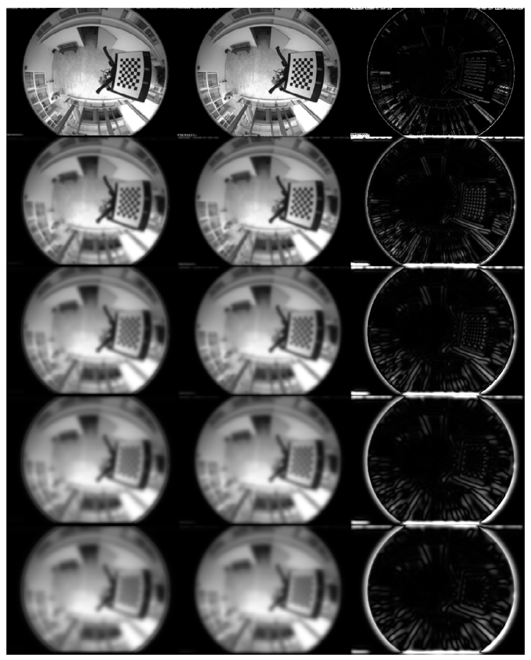
The results of Algorithm 2 for an image of the calibrated fisheye camera are shown in Figure 11 for iteration k = 1 (first row), k = 10, k = 20, k = 30 and k = 40 (last row). The left column shows the result of Algorithm 2 (using the geodetically defined Gaussian kernel), the middle column the response of the classic Gaussian kernel and the right column the absolute difference, scaled for visualization purposes.

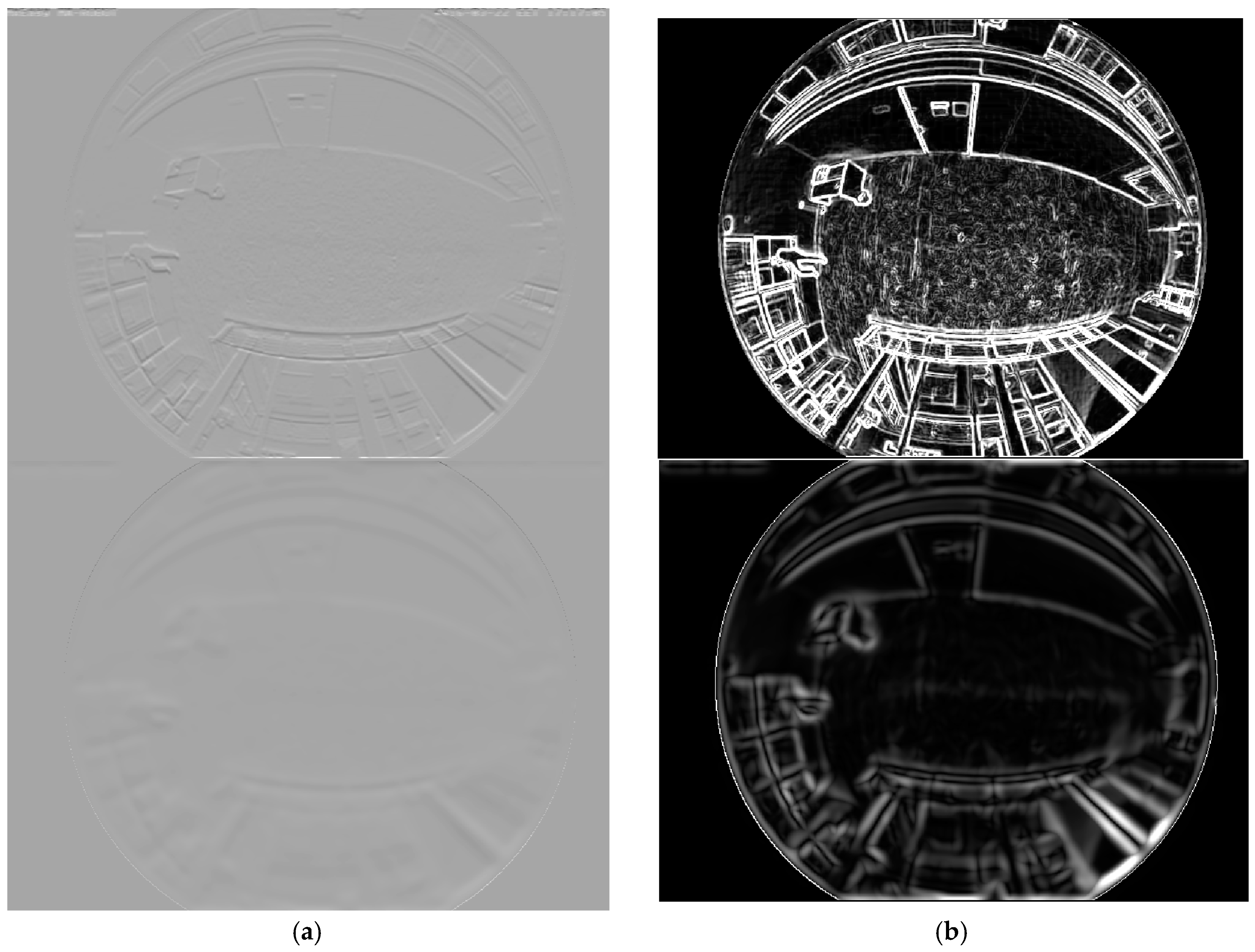
Results of the response of the geodesic g_x kernel, as approximated using Algorithm 2 and Equation (18), for iteration k = 1 and k = 20 are shown in Figure 12 (left column). In the right column the magnitude of the image gradient is shown, using the responses of the two partial derivatives of the geodetic Gaussian kernel. It is evident that for small value of σ = σ₀, fine details appear in the magnitude of the gradient, whereas, in the case of k = 20 (thus σ = ${\mathsf{\sigma }}_0\sqrt{21}$), only thick lines appear in the magnitude of the gradient image.

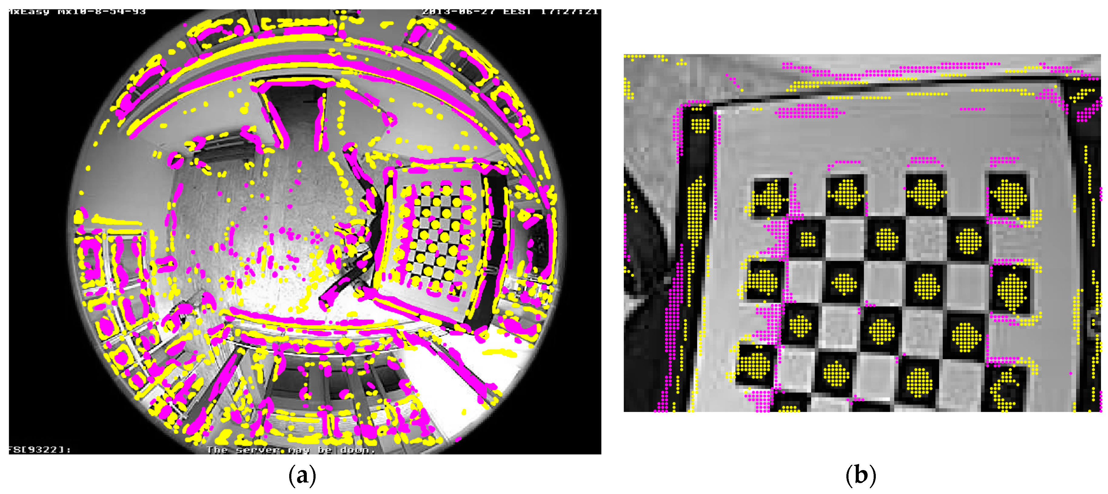
The results of the maximum response of the normalized geodetically corrected LoG, approximated by DoG (Algorithm 3) are shown in Figure 13. The initial Gaussian kernel g₀ was defined over a 7 × 7 window and 40 iterations were executed. Yellow indicates pixels that exhibited maximum DoG response within the first 4 iterations, whereas magenta indicates pixels with maximum DoG response between 5 and 10 iterations. In (a) the whole fisheye frame is displayed, whereas in (b) details are shown for a zoomed portion of the image.

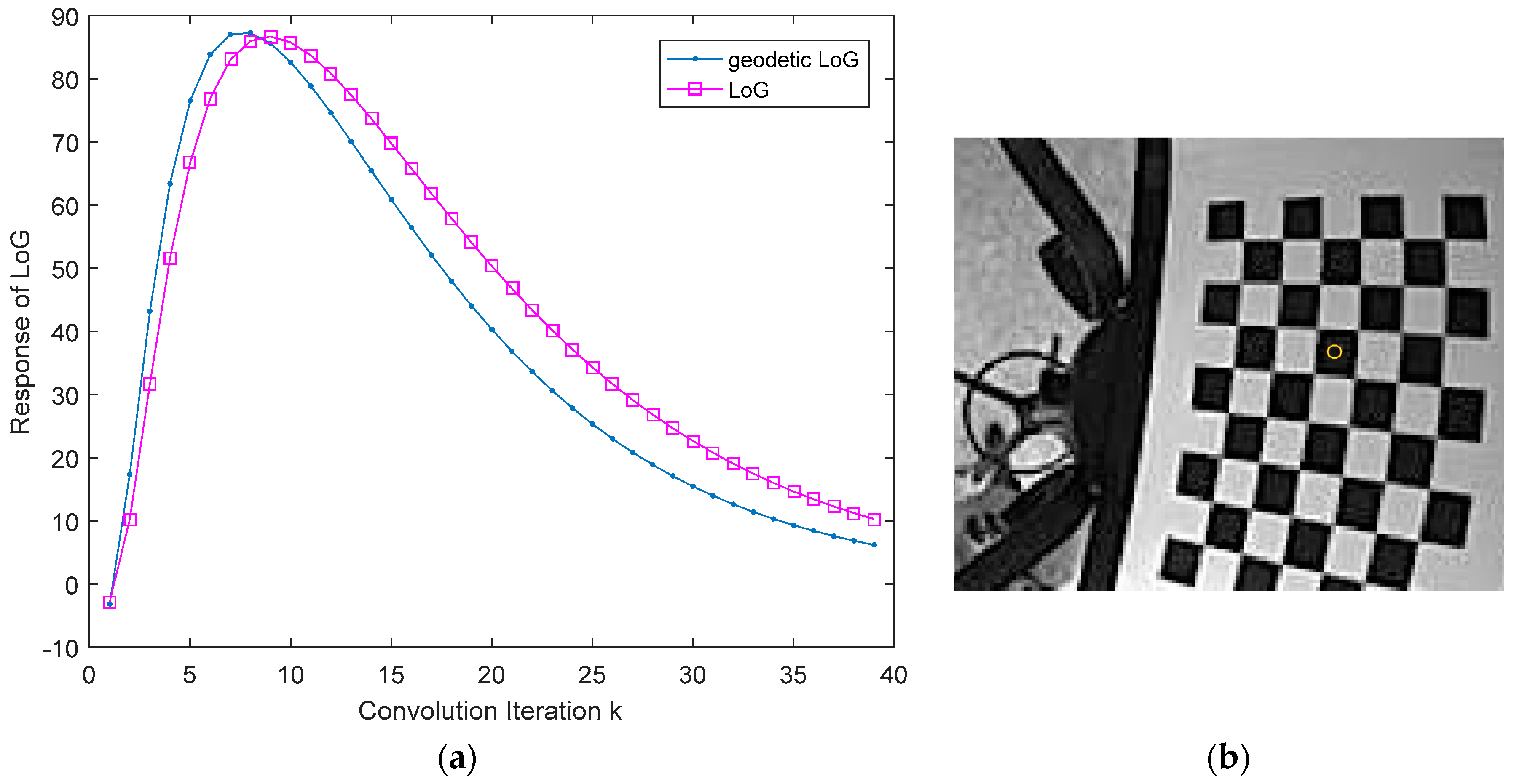
A comparison between the classic LoG response and the response of the geodetically defined LoG, approximated by the DoG, (after normalization in both cases) is given in Figure 14a. The curves have been produced for the pixel shown in the image portion of Figure 14b.

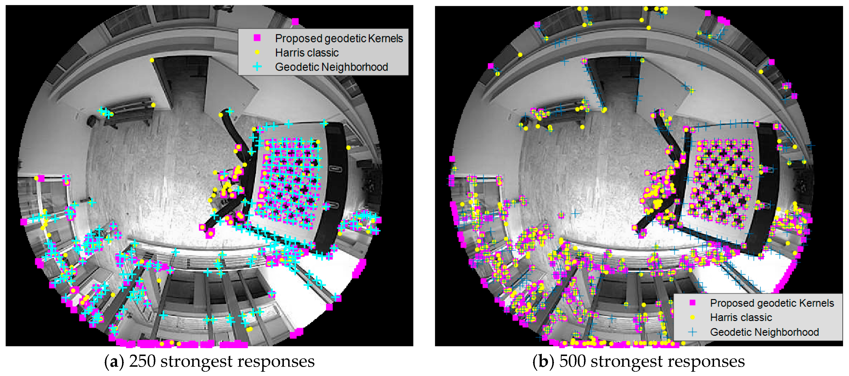
The response of Harris corner detection is shown in Figure 15 for the whole frame. Yellow dots indicate corners detected by the proposed geodetic Harris detector, whereas magenta squares depict corner pixels detected by the classic Harris detector and blue crosses are corners detected by the method described in [22]. All detectors were applied for a number of different image scales. Common image scale is determined by the size of the kernels. In the results presented in this section, the initial small geodetic Gaussian is set to a size of 5 × 5 pixels. The size of the equivalent kernel after the subsequent convolutions is shown in

Table 1. Quantitative evaluation, in terms of corner detection, of the proposed geodetic kernel definition, the geodetic neighborhood definition in [22] and classic Harris-based corner detection. The number of correctly detected corners in the chessboard (80 corners in total) by each method, considering the 250 strongest responses are shown.

Kernel Size	Classic Harris	Proposed Geodetic Kernels	Geodetic Neighborhood [22]
5 × 5	76	80	80
9 × 9	80	80	80
13 × 13	75	80	80
17 × 17	53	80	80
21 × 21	48	80	80

and

Table 2. False corner detection of the proposed geodetic kernel definition, the geodetic neighborhood definition in [22] and classic Harris-based corner detection. The number of wrongly detected corners by each method, considering the 250 and 500 strongest responses are shown.

Kernel Size	250 Strongest Corner Responses			500 Strongest Corner Responses
	Classic Harris	Proposed Geodetic Kernels	Geodetic Neighborhood [22]	Classic Harris	Proposed Geodetic Kernels	Geodetic Neighborhood [22]
5 × 5	9	2	21	11	4	68
9 × 9	10	1	31	35	5	72
13 × 13	12	2	17	42	7	69
17 × 17	19	4	28	70	8	72
21 × 21	28	8	27	68	12	65

. The classic Harris-based corner detection is applied using this size for the integration Gaussian kernel (which is slightly larger than the differentiating Gaussian). The geodetic neighborhood method [22] is parameterized by the kernel’s field of view, measured in radians or degrees and the number of pixels of the kernel’s stencil. After visually studying the image resampling that is required by this method (an example is shown in Figure 6d) the selected parameterization was as following: a field of view (FoV) of 1 degree was used for 5 × 5 and 9 × 9 and an FoV of 2 degrees for the larger kernels. The numerical assessment of the methods is two-fold. First the 250 strongest corner responses are considered and the number of correctly identified corners in the chessboard are enumerated. The chessboard contains 80 corners. The results are presented in Table 1. The zoomed chessboard areas are shown in Figure 15 for the first four kernel sizes of Table 1. Secondly, the number of wrong corner responses is measured by visual inspection for all three methods, for four (4) different kernel sizes (equivalently, image scales). The results are measured considering the 250, as well as the 500 strongest corner responses from each method. The results are presented in Table 2.

Two different parts of the fisheye frame are zoomed in Figure 16. Visual inspection of the results suggests that the proposed geodetic Harris detector has fewer false corners than the classic one. Figure 17 shows a few sporadic false corners detected by the classic Harris method, probably due to the texture of the floor. The method of [22] exhibits false detections mainly on image edges.

The presented results can be summarized as following. The proposed definition and implementation of image processing geodetic kernels exhibited very good corner detection over a number of different kernel sizes: it managed to detect all corners in the chessboard area for kernel size ranging between 5 × 5 to 21 × 21 pixels. The same holds for the method of geodetic image neighborhood resampling [22]. On the other hand, the classic Harris-based corner detection does not perform well on the fisheye images when the size of the kernels (image space) increases. Concerning false corner detection, the proposed algorithm achieved very low rate for the 5 different kernel sizes that it was tested. On the contrary, the classic Harris-based detector exhibited increased false detection rate as the kernel size increases, whereas the method of [22] exhibited high false detection rate for almost all tested kernel sizes.

The main algorithms described in this work have been executed on a laptop with Intel core i7-7700 HQ, 16 GB, with Windows 10, using the Matlab programming environment. The algorithms were applied to 480 × 640 fisheye images. The recorded times of various steps of the methods are shown in

Table 3. Execution times for the proposed method, corner detection in [22] and classic corner detection.

Method	Calculation	Execution Time (Second)
Proposed Geodetic kernels	geodetic Gaussian g0 (Algorithm 1)	5.5
Geodetic neighborhood [22]	Image resampling, 5 × 5, FoV 1°	150
Proposed Geodetic kernels	Gaussian response (Algorithm 2)	0.15
Geodetic neighborhood [22]	Gaussian response	0.017
Classic Harris	Gaussian response	0.017
Proposed Geodetic kernels	Harris Matrix M	0.5
Classic Harris	Harris Matrix M	0.5
Geodetic neighborhood [22]	Harris Matrix M	0.5

. It has to be mentioned again that the slowest part of the proposed algorithm, the initial calculation of the geodetic Gaussian kernel g₀ with small σ₀ (first entry in Table 3) is executed only once, after the calibration of the camera and it can be subsequently used for any image acquired by the specific camera. As it can be observed in Table 3, Algorithm 1 is the computationally intensive part of the proposed method. Execution times using the classic kernels are also provided for comparison. The geodetic approach for fisheye image processing using geodetic neighborhood [22] has also been timed. The slowest part of the method is the image resampling, which was timed for the following parameterization: FoV of 1 degree, kernel size of 5 × 5. Increasing the FoV and consequently the kernel size imposes a significant overhead to the algorithm [22]. Furthermore, this operation has to be performed for every acquired image.

4. Discussion

In this work, the most important image processing kernels, namely, the Gaussian, its partial derivatives with respect to x and y and the Laplacian of Gaussian (LoG) have been redefined for a calibrated fisheye camera, using the geodesic distance between pixels, of the fisheye image. For each kernel, a computationally efficient algorithm that calculates/approximates the response with a fisheye image acquired by a calibrated camera, based on successive convolutions with a small pre-initialized geodetic Gaussian, has been presented. The Harris corner detection has also been implemented for a calibrated fisheye camera, using the image responses with the redefined geodetic kernels. The results show that the proposed definitions and the computational implementations are efficient and present subtle differences from the applications of the classic image processing kernels. Corner detection in calibrated fisheye images appears more robust when using the proposed operators. More specifically, both the proposed method of geodetic definition of image processing kernels and the method of geodetic image neighborhood resampling achieved very high corner detection for all tested kernel sizes. The performance of the classic Harris-based corner detector, deteriorates as the kernel size increases. The number of falsely indicated corners is much lower for the proposed method, consistently for all tested kernel sizes. The geodetic neighborhood method [22] is producing a large number of false corner detections over all tested kernel sizes, whereas the classic corner detector exhibited false detection rate that deteriorates as the kernel size increases.

The execution time of the proposed method was slower than the corresponding time using the classic kernels, but not prohibitive for practical use. The most demanding step was the initial calculation of the initial geodetic Gaussian g₀ with small σ₀, which needs only be performed once, after camera calibration. The approximation of the Gaussian response which was averaged to 0.017 s per iteration for a 480 × 640 image. Possible parallel of this step may achieve important acceleration. Further work is needed to expand these results into more image analysis/feature extraction methods from fisheye images.

References

- Geyer, C.; Daniilidis, K. Catadioptric projective geometry. Int. J. Comput. Vis. 2001, 45, 223–243. [Google Scholar] [CrossRef]
- Bermudez-Cameo, J.; Lopez-Nicolas, G.; Guerrero, J.J. Automatic line extraction in uncalibrated omnidirectional cameras with revolution symmetry. Int. J. Comput. Vis. 2015, 114, 16–37. [Google Scholar] [CrossRef]
- Ahmed, M.S.; Gao, Z. Ultra-wide fast fisheye for security and monitoring applications. In Proceedings of the International Symposium on Optoelectronic Technology and Application 2014: Advanced Display Technology; and Nonimaging Optics: Efficient Design for Illumination and Solar Concentration, Beijing, China, 13–15 May 2014. [Google Scholar]
- Caruso, D.; Engel, J.; Cremers, D. Large-scale direct slam for omnidirectional cameras. In Proceedings of the 2015 IEEE/RSJ International Conference on Intelligent Robots and Systems (IROS), Hamburg, Germany, 28 September–2 October 2015; pp. 141–148. [Google Scholar]
- Choi, Y.W.; Kwon, K.K.; Lee, S.I.; Choi, J.W.; Lee, S.G. Multi-robot Mapping Using Omnidirectional-Vision SLAM Based on Fisheye Images. ETRI J. 2014, 36, 913–923. [Google Scholar] [CrossRef]
- Abrams, A.D.; Pless, R.B. Webcams in context: Web interfaces to create live 3D environments. In Proceedings of the 18th ACM International Conference on Multimedia, Toronto, ON, Canada, 26–30 October 2010; pp. 331–340. [Google Scholar]
- Sankaranarayanan, K.; Davis, J.W. A fast linear registration framework for multi-camera GIS coordination. In Proceedings of the IEEE International Conference on Advanced Video and Signal Based Surveillance, Santa Fe, NM, USA, 1–3 September 2008. [Google Scholar]
- Hu, X.; Zheng, H.; Chen, Y.; Chen, L. Dense crowd counting based on perspective weight model using a fisheye camera. Optik-Int. J. Light Electron Opt. 2015, 126, 123–130. [Google Scholar] [CrossRef]
- Vandewiele, F.; Motamed, C.; Yahiaoui, T. Visibility management for object tracking in the context of a fisheye camera network. In Proceedings of the 2012 Sixth International Conference on Distributed Smart Cameras (ICDSC), Hong Kong, China, 30 October–2 November 2012; pp. 1–6. [Google Scholar]
- Wang, W.; Gee, T.; Price, J.; Qi, H. Real time multi-vehicle tracking and counting at intersections from a fisheye camera. In Proceedings of the 2015 IEEE Winter Conference on Applications of Computer Vision (WACV), Waikoloa, HI, USA, 5–9 January 2015; pp. 17–24. [Google Scholar]
- Rhodin, H.; Richardt, C.; Casas, D.; Insafutdinov, E.; Shafiei, M.; Seidel, H.P.; Theobalt, C. Egocap: Egocentric marker-less motion capture with two fisheye cameras. ACM Trans. Graph. 2016, 35, 162. [Google Scholar] [CrossRef]
- Rhodin, H.; Robertini, N.; Richardt, C.; Seidel, H.P.; Theobalt, C. A versatile scene model with differentiable visibility applied to generative Pose Estimation. In Proceedings of the 2015 International Conference on Computer Vision (ICCV 2015), Tampa, FL, USA, 5–8 December 2015. [Google Scholar]
- Lowe, D.G. Object recognition from local scale-invariant features. In Proceedings of the Seventh IEEE International Conference on Computer Vision, Kerkyra, Greece, 20–27 September 1999; Volume 2, pp. 1150–1157. [Google Scholar]
- Hansen, P.; Corke, P.; Boles, W.; Daniilidis, K. Scale Invariant Feature Matching with Wide Angle Images. In Proceedings of the IEEE/RSJ International Conference on Intelligent Robots and Systems, San Diego, CA, USA, 29 October–2 November 2007; pp. 1689–1694. [Google Scholar]
- Bulow, T. Spherical diffusion for 3D surface smoothing. IEEE Trans. Pattern Anal. Mach. Intell. 2004, 26, 1650–1654. [Google Scholar] [CrossRef] [PubMed]
- Cruz-Mota, J.; Bogdanova, I.; Paquier, B.; Bierlaire, M.; Thiran, J.P. Scale invariant feature transform on the sphere: Theory and applications. Int. J. Comput. Vis. 2012, 98, 217–241. [Google Scholar] [CrossRef]
- Puig, L.; Guerrero, J.J. Scale space for central catadioptric systems: Towards a generic camera feature extractor. In Proceedings of the 2011 IEEE International Conference on Computer Vision (ICCV), Barcelona, Spain, 6–13 November 2011; pp. 1599–1606. [Google Scholar]
- Puig, L.; Guerrero, J.J.; Daniilidis, K. Scale space for camera invariant features. IEEE Trans. Pattern Anal. Mach. Intell. 2014, 36, 1832–1846. [Google Scholar] [CrossRef] [PubMed]
- Andreasson, H.; Treptow, A.; Duckett, T. Localization for mobile robots using panoramic vision, local features and particle filter. In Proceedings of the 2005 IEEE International Conference on Robotics and Automation, Barcelona, Spain, 18–22 April 2005; pp. 3348–3353. [Google Scholar]
- Zhao, Q.; Feng, W.; Wan, L.; Zhang, J. SPHORB: A fast and robust binary feature on the sphere. Int. J. Comput. Vis. 2015, 113, 143–159. [Google Scholar] [CrossRef]
- Hara, K.; Inoue, K.; Urahama, K. Gradient operators for feature extraction from omnidirectional panoramic images. Pattern Recognit. Lett. 2015, 54, 89–96. [Google Scholar] [CrossRef]
- Demonceaux, C.; Vasseur, P.; Fougerolle, Y. Central catadioptric image processing with geodesic metric. Image Vis. Comput. 2011, 29, 840–849. [Google Scholar] [CrossRef]
- Delibasis, K.K.; Plagianakos, V.P.; Maglogiannis, I. Refinement of human silhouette segmentation in omni-directional indoor videos. Comput. Vis. Image Underst. 2014, 128, 65–83. [Google Scholar] [CrossRef]
- Delibasis, K.K.; Georgakopoulos, S.V.; Kottari, K.; Plagianakos, V.P.; Maglogiannis, I. Geodesically-corrected Zernike descriptors for pose recognition in omni-directional images. Integr. Comput.-Aided Eng. 2016, 23, 185–199. [Google Scholar] [CrossRef]
- Puig, L.; Bermúdez, J.; Sturm, P.; Guerrero, J.J. Calibration of omnidirectional cameras in practice: A comparison of methods. Comput. Vis. Image Underst. 2012, 116, 120–137. [Google Scholar] [CrossRef]
- Harris, C.; Stephens, M. A combined corner and edge detector. In Proceedings of the Alvey Vision Conference, Manchester, UK, 31 August–2 September 1988; Volume 15, pp. 10–5244. [Google Scholar]
- Mokhtarian, F.; Mohanna, F. Performance evaluation of corner detectors using consistency and accuracy measures. Comput. Vis. Image Underst. 2006, 102, 81–94. [Google Scholar] [CrossRef]
Figure 1.
A typical image from a roof-based fisheye camera.
Figure 2.
The resulting calibration of the fisheye camera, for each image pixel (a) the azimuthal angle θ and (b) the elevation angle φ is provided.
Figure 3.
The basic concept of fisheye image formation, involving a (semi) spherical lens and central projection on the image plane. The difference between Euclidean distance between pixels on the image plane and geodesic distance (on the spherical lens) becomes apparent.
Figure 4.
Graphic representation of Dx (left) and Dy (right).
Figure 5.
The Gaussian defined in Equation (9) at different positions on the fisheye image, using the geodetic distance is shown in (a) 3D and (b) as color-encoded image.