Full Reference Objective Quality Assessment for Reconstructed Background Images


School of Electrical, Computer and Energy Engineering, Arizona State University, Tempe, AZ 85287, USA
*
Author to whom correspondence should be addressed.
J. Imaging 2018, 4(6), 82; https://doi.org/10.3390/jimaging4060082
Submission received: 16 May 2018
/
Revised: 6 June 2018
/
Accepted: 6 June 2018
/
Published: 19 June 2018
(This article belongs to the Special Issue Detection of Moving Objects)
Abstract
:With an increased interest in applications that require a clean background image, such as video surveillance, object tracking, street view imaging and location-based services on web-based maps, multiple algorithms have been developed to reconstruct a background image from cluttered scenes. Traditionally, statistical measures and existing image quality techniques have been applied for evaluating the quality of the reconstructed background images. Though these quality assessment methods have been widely used in the past, their performance in evaluating the perceived quality of the reconstructed background image has not been verified. In this work, we discuss the shortcomings in existing metrics and propose a full reference Reconstructed Background image Quality Index (RBQI) that combines color and structural information at multiple scales using a probability summation model to predict the perceived quality in the reconstructed background image given a reference image. To compare the performance of the proposed quality index with existing image quality assessment measures, we construct two different datasets consisting of reconstructed background images and corresponding subjective scores. The quality assessment measures are evaluated by correlating their objective scores with human subjective ratings. The correlation results show that the proposed RBQI outperforms all the existing approaches. Additionally, the constructed datasets and the corresponding subjective scores provide a benchmark to evaluate the performance of future metrics that are developed to evaluate the perceived quality of reconstructed background images.
1. Introduction
A clean background image has great significance in multiple applications. It can be used for video surveillance [1], activity recognition [2], object detection and tracking [3,4], street view imaging and location-based services on web-based maps [5,6], and texturing 3D models obtained from multiple photographs or videos [7]. However, acquiring a clean photograph of a scene is seldom possible. There are always some unwanted objects occluding the background of interest. The technique of acquiring a clean background image by removing the occlusions using frames from a video or multiple views of a scene is known as background reconstruction or background initialization. Many algorithms have been proposed for initializing the background images from videos, for example [8,9,10,11,12,13,14]; and also from multiple images such as [15,16,17].
Background initialization or reconstruction is crippled by multiple challenges. The pseudo-stationary background (e.g., waving trees, waves in water, etc.) poses additional challenges in separating the moving foreground objects from the relatively stationary background pixels. The illumination conditions can vary across the images, thus changing the global characteristics of each image. The illumination changes cause local phenomena such as shadows, reflections and shading, which change the local characteristics of the background across the images or frames in a video. Finally, the removal of ‘foreground’ objects from the scene creates holes in the background that need to be filled in with pixels that maintain the continuity of the background texture and structures in the recovered image. Thus, the background reconstruction algorithms can be characterized by two main tasks:
- (1)
- foreground detection, in which the foreground is separated from the background by classifying pixels as foreground or background;
- (2)
- background recovery, in which the holes formed due to foreground removal are filled.
The performance of a background extraction algorithm depends on two factors:
- (1)
- its ability to detect the foreground objects in the scene and completely eliminate them; and
- (2)
- the perceived quality of the reconstructed background image.
Traditional statistical techniques such as Peak Signal to Noise Ratio (PSNR), Average Gray-level Error (AGE), total number of error pixels (EPs), percentage of EPs (pEP), number of Clustered Error Pixels (CEPs) and percentage of CEPs (pCEPs) [18] quantify the performance of the algorithm in its ability to remove foreground objects from a scene to a certain extent, but they do not give an indication of the perceived quality of the generated background image. On the other hand, the existing Image Quality Assessment (IQA) techniques such as Multi-scale Similarity metric (MS-SSIM) [19] and Color image Quality Measures (CQM) [20] used by the authors in [21] to compare different background reconstruction algorithms are not designed to identify any residual foreground objects in the scene. Lack of a quality metric that can reliably assess the performance of background reconstruction algorithms by quantifying both aspects of a reconstructed background image motivated the development of the proposed Reconstructed Background visual Quality Index (RBQI). The proposed RBQI is a full-reference objective metric that can be used by background reconstruction algorithm developers to assess and optimize the performance of their developed methods and also by users to select the best performing method. Research challenges such as the Scene Background Modeling Challenge (SBMC) 2016 [22] are also in need of a reliable objective scoring measure. RBQI uses the contrast, structure and color information to determine the presence of any residual foreground objects in the reconstructed background image as compared to the reference background image and to detect any unnaturalness introduced by the reconstruction algorithm that affects the perceived quality of the reconstructed background image.
This paper also presents two datasets that are constructed to assess the performance of the proposed as well as popular existing objective quality assessment methods in predicting the perceived visual quality of the reconstructed background images. The datasets consist of reconstructed background images generated using different background reconstruction algorithms in the literature along with the corresponding subjective ratings. Some of the existing datasets such as video surveillance datasets (Wallflower [23], I2R [3]), background subtraction datasets (UCSD [24], CMU [25]) and object tracking evaluation dataset (“Performance Evaluation of Tracking and Surveillance (PETS)") are not suited for benchmarking the background reconstruction algorithms or the objective quality metrics used for evaluating the perceived quality of reconstructed background images as they do not provide reconstructed background images as ground-truth. The more recent dataset “Scene Background Modeling Net” (SBMNet) [26,27] is targeted at comparing the performance of the background initialization algorithms. It provides the reconstructed images as ground truth, but it does not provide any subjective ratings for these images. Hence, the SBMNet dataset [26,27] is not suited for benchmarking the performance of objective background visual quality assessment. Thus, the datasets proposed in this work are the first and currently the only datasets that can be used for benchmarking existing and future metrics developed to assess the quality of reconstructed background images. The constructed datasets and the code for RBQI are available for download at Supplementary Materials.
The rest of the paper is organized as follows. In Section 2, we highlight the limitations of existing popular assessment methods [28]. We introduce the new benchmarking datasets in Section 3 along with the details of the subjective tests. In Section 4, we propose a new index that makes use of a probability summation model to combine structure and color characteristics at multiples scales for quantifying the perceived quality in reconstructed background images. Performance evaluation results for the existing and proposed objective visual quality assessment methods are presented in Section 5 for reconstructed background images. Finally, we conclude the paper in Section 6 and also provide directions for future research.
2. Existing Full Reference Background Quality Assessment Techniques and Their Limitations
Existing background reconstruction quality metrics can be classified into two categories: statistical and image quality assessment (IQA) techniques, depending on the type of features used for measuring the similarity between the reconstructed background image and reference background image.
2.1. Statistical Techniques
Statistical techniques use intensity values at co-located pixels in the reference and reconstructed background images to measure the similarity. Popular statistical techniques [18] that have been traditionally used for judging the performance of background initialization algorithms are briefly explained here:
- (i)
- Average Gray-level Error (): AGE is calculated as the absolute difference between the gray levels of the co-located pixels in the reference and reconstructed background image.
- (ii)
- Error Pixels (): gives the total number of error pixels. A pixel is classified as an error pixel if the absolute difference between the corresponding pixels in the reference and reconstructed background images is greater than an empirically selected threshold .
- (iii)
- Percentage Error Pixels (): Percentage of the error pixels, calculated as EP/N, where N is the total number of pixels in the image.
- (iv)
- Clustered Error Pixels (): gives the total number of clustered error pixels. A clustered error pixel is defined as the error pixel whose four connected pixels are also classified as error pixels.
- (v)
- Percentage Clustered Error Pixels (): Percentage of the clustered error pixels, calculated as CEP/N, where N is the total number of pixels in the image.
Though these techniques were used in the literature to assess the quality of reconstructed background images, their performance was not previously evaluated. As we show in Section 5 and as noted by the authors in [28], the statistical techniques were found to not correlate well with the subjective quality scores in terms of prediction accuracy and prediction consistency.
2.2. Image Quality Assessment Techniques
The existing Full Reference Image Quality Assessment (FR-IQA) techniques use perceptually inspired features for measuring the similarity between two images. Though these techniques have been shown to work reasonably well while assessing images affected by distortions such as blur, compression artifacts and noise, these techniques have not been designed for assessing the quality of reconstructed background images.
In [21,27], popular FR-IQA techniques including Peak Signal to Noise Ratio (PSNR), Multi-Scale Similarity (MS-SSIM) [19] and Color image Quality Measure (CQM) [20] were adopted for objectively comparing the performance of the different background reconstruction algorithms; however, no performance evaluation was carried out to support the choice of these techniques. Other popular IQA techniques include Structural Similarity Index (SSIM) [29], visual signal-to-noise ratio (VSNR) [30], visual information fidelity (VIF) [31], pixel-based VIF (VIFP) [31], universal quality index (UQI) [32], image fidelity criterion (IFC) [33], noise quality measure (NQM) [34], weighted signal-to-noise ratio (WSNR) [35], feature similarity index (FSIM) [36], FSIM with color (FSIMc) [36], spectral residual based similarity (SR-SIM) [37] and saliency-based SSIM (SalSSIM) [38]. A review of existing FR-IQA techniques is presented in [39,40,41]. The suitability of these techniques for evaluating the quality of reconstructed background images remains unexplored.
As the first contribution of this paper, we present two benchmarking datasets that can be used for comparing the performance of different techniques in objectively assessing the perceived quality of the reconstructed background images. These datasets contain reconstructed background images along with their subjective ratings, details of which are discussed in Section 3.1. A preliminary version of the benchmarking dataset discussed in Section 3.1.1 was published in [28]. In this paper, we provide an additional larger dataset as described in Section 3.1.2. We also propose a novel objective Reconstructed Background Quality Index (RBQI) that is shown to outperform existing techniques in assessing the perceived visual quality of reconstructed background images.
3. Subjective Quality Assessment of Reconstructed Background Images
3.1. Datasets
In this section, we present two different datasets constructed as part of this work to serve as benchmarks for comparing existing and future techniques developed for assessing the quality of reconstructed background images. The images and subjective experiments for both datasets are described in the subsequent subsections.
Each dataset contains the original sequence of images or videos that are used as inputs to the different reconstruction algorithms, the background images reconstructed by the different algorithms and the corresponding subjective scores. For details on the algorithms used to reconstruct the background images, the reader is referred to [27,28].
3.1.1. Reconstructed Background Quality (ReBaQ) Dataset
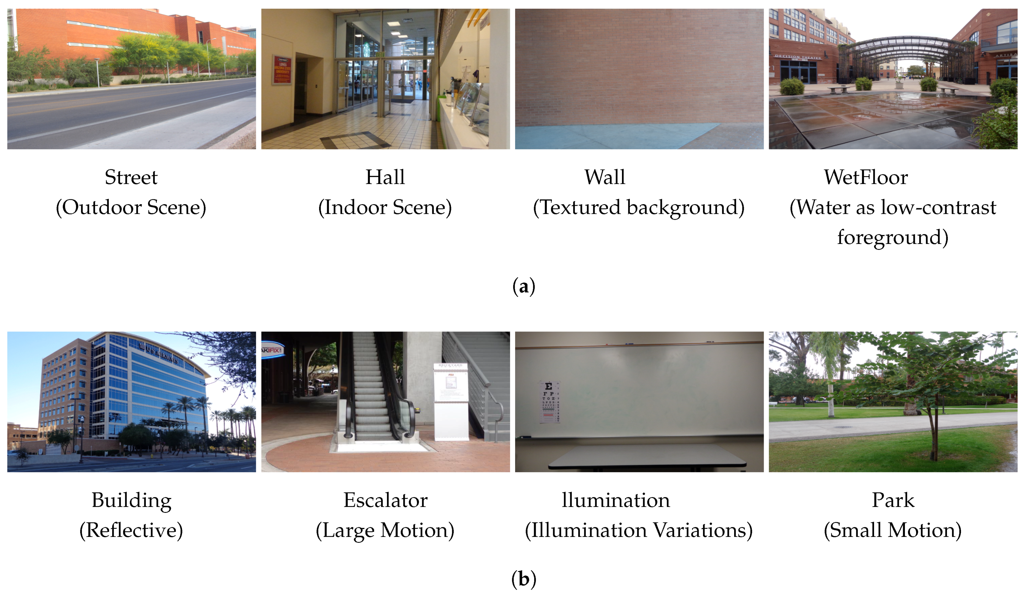
This dataset consists of eight different scenes. Each scene consists of a sequence of eight images where every image is a different view of the scene captured by a stationary camera. Each image sequence is captured such that the background is visible at every pixel in at least one of the views. A reference background image that is free of any foreground objects is also captured for every scene. Figure 1 shows the reference images corresponding to each of the eight different scenes in this dataset. The spatial resolution of the sequence corresponding to each of the scenes is 736 × 416.
Each of the image sequences is used as input to twelve different background reconstruction algorithms [8,9,10,11,12,13,14,15,16,17]. The default settings as suggested by the authors in the respective papers were used for generating the background images. For the block-based algorithms of [11,14] and [17], the block sizes are set to 8, 16 and 32 to take into account the effect of varying block sizes on the perceived quality of the recovered background. As a result, 18 background images are generated for each of the eight scenes. These 144 reconstructed background images along with the corresponding reference images for the scene are then used for the subjective evaluation. Each of the scenes pose a different challenge for the background reconstruction algorithms. For example, “Street” and “Wall” are outdoor sequences with textured backgrounds while “Hall” is an indoor sequence with textured background. The “WetFloor” sequence challenges the underlying principal of many background reconstruction algorithms with water appearing as a low-contrast foreground object. The “Escalator” sequence has large motion in the background due to the moving escalator, while “Park” has smaller motion in the background due to waving trees. The “Illumination” sequence exhibits changing light sources, directions and intensities while the “Building” sequence has changing reflections in the background. Broadly, the dataset contains two categories based on the scene characteristics: (i) Static, the scenes for which all the pixels in the background are stationary; and (ii) Dynamic, the scenes for which there are non-stationary background pixels (e.g., moving escalator, waving trees, varying reflections). Four out of the eight scenes in the ReBaQ dataset are categorized as Static and the remaining four are categorized as Dynamic scenes. The reference background images corresponding to the static scenes are shown in Figure 1a. Although there are reflections on the floor in the “WetFloor” sequence, it does not exhibit variations at the time of recording and hence it is categorized as a static background scene. The reference background images corresponding to the dynamic background scenes are shown in Figure 1b.
3.1.2. SBMNet Based Reconstructed Background Quality (S-ReBaQ) Dataset
This dataset is created from the videos in the Scene Background Modeling Net (SBMNet) dataset [26] used for the Scene Background Modeling Challenge (SBMC) 2016 [22]. SMBNet consists of image sequences corresponding to a total of 79 scenes. These image sequences are representative of typical indoor and outdoor visual data captured in surveillance, smart environment, and video dataset scenarios. The spatial resolutions of the sequences corresponding to different scenes vary from 240 × 240 to 800 × 600. The length of the sequences also varies from 6 to 9370 images. The authors of SBMNet categorize these scenes into eight different classes based on the challenges posed [26]: (a) the Basic category represents a mixture of mild challenges typical of the shadows, Dynamic Background, Camera Jitter and Intermittent Object Motion categories; (b) the Background motion category includes scenes with strong (parasitic) background motion; for example, in the “Advertisement Board” sequence, the advertisement board in the scene periodically changes; (c) the Intermittent Motion category includes sequences with scenarios known for causing “ghosting” artifacts in the detected motion; (d) the Jitter category contains indoor and outdoor sequences captured by unstable cameras; (e) the Clutter category includes sequences containing a large number of foreground moving objects occluding a large portion of the background; (f) the Illumination Changes category contains indoor sequences containing strong and mild illumination changes; (g) the Very Long category contains sequences each with more than 3500 images; and (h) the Very Short category contains sequences with a limited number of images (less than 20). The authors of SBMNet [26] provide reference background images for only 13 scenes out of the 79 scenes. There is at least one scene corresponding to each category with reference background image available. We use only these 13 scenes for which the reference background images are provided. Figure 2 shows the reference background images corresponding to the scenes in this dataset with the categories from SBMNet [26,27] in brackets. Background images that were reconstructed by 14 algorithms submitted to SBMC [12,16,42,43,44,45,46,47,48,49,50,51] corresponding to the selected 13 scenes were used in this work for conducting subjective tests. As a result, a total of 182 () reconstructed background images along with their corresponding subjective scores form the S-ReBaQ dataset.
3.2. Subjective Evaluation
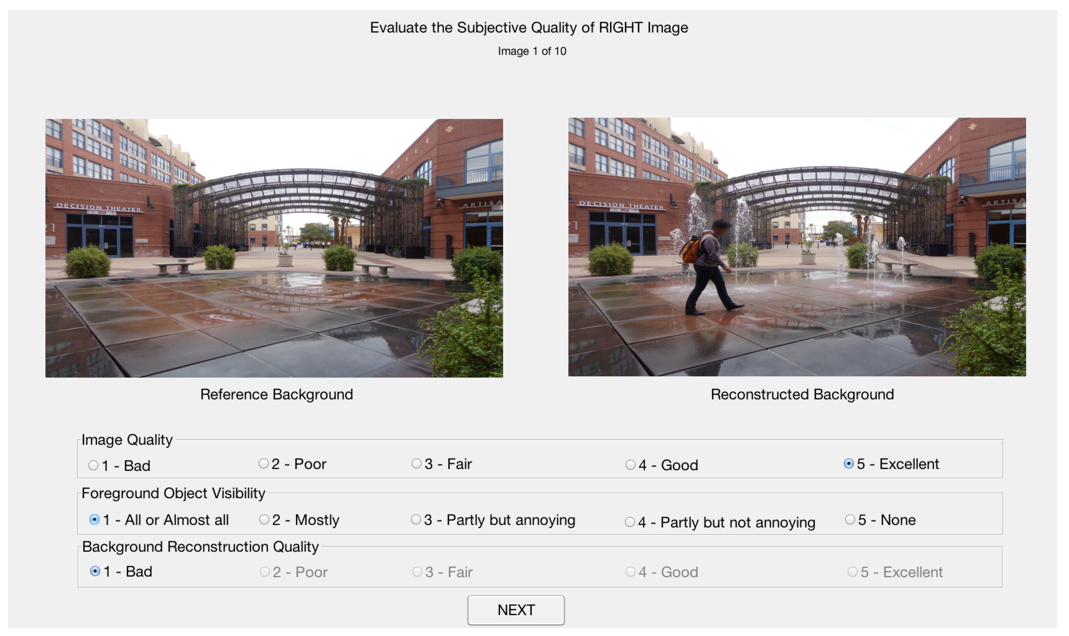
The subjective ratings are obtained by asking the human subjects to rate the similarity of the reconstructed background images to the reference background images. The subjects had to score the images based on three aspects: (1) overall perceived visual image quality; (2) visibility or presence of foreground objects; and (3) perceived background reconstruction quality. The subjects had to score the image quality on a 5-point scale, with 1 being assigned to the lowest rating of ‘Bad’ and 5 assigned to the highest rating of ‘Excellent’. The second aspect was determining the presence of foreground objects. For our application, we defined the foreground object as any object that is not present in the reference image. The foreground visibility was scored on a 5-point scale marked as: ‘1—All foreground visible’, ‘2—Mostly visible’, ‘3—Partly visible but annoying’, ‘4—Partly visible but not annoying’ and ‘5—None visible’. The background reconstruction quality was also measured using a 5-point scale similar to that of the image quality, but the choices were limited based on how the first two aspects of an image were scored. If either the image quality or foreground object visibility was rated 2 or less, the highest possible score for background reconstruction quality was restricted to the minimum of the two scores. For example, as illustrated in Figure 3, if the image quality was rated as excellent, but the foreground object visibility was rated 1 (all visible), the reconstructed background quality cannot be scored to be very high. Choices for background reconstruction quality rating were not restricted for any other image quality and foreground object visibility scores. The background reconstruction quality scores, referred to as raw scores in the rest of the paper, are used for calculating the Mean Opinion Score (MOS).
We adopted a double-stimulus technique in which the reference and the reconstructed background images were presented side-by-side [52] to each subject as shown in Figure 3. Though the same testing strategy and set up was used for the ReBaQ and S-ReBaQ datasets described in Section 3.1, the tests for each dataset were conducted in separate sessions.
As discussed in [28], the subjective experiments were carried out on a 23-inch Alienware monitor with a resolution of 1920 × 1080. Before the experiment, the monitor was reset to its factory settings. The setup was placed in a laboratory under normal office illumination conditions. Subjects were asked to sit at a viewing distance of 2.5 times the monitor height.
Seventeen subjects participated in the subjective test for the ReBaQ dataset, while sixteen subjects participated in the subjective test for the S-ReBaQ dataset. The subjects were tested for vision and color blindness using the Snellen chart [53] and Ishihara color vision test [54], respectively. A training session was conducted before the actual subjective testing, in which the subjects were shown a few images covering different quality levels and distortions of the reconstructed background images and their responses were noted to confirm their understanding of the tests. The images used during training were not included in the subjective tests.
Since the number of participating subjects was less than 20 for each of the datasets, the raw scores obtained by subjective evaluation were screened using the procedure in ITU-R BT 500.13 [52]. The kurtosis of the scores is determined as the ratio of the fourth order moment and the square of the second order moment. If the kurtosis lies between 2 and 4, the distribution of the scores can be assumed to be normal. If more than 5% of the scores given by a particular subject lie outside the range of two standard deviations from the mean scores in case of normally distributed scores, this subject is rejected. For the scores that are not normally distributed, the range is determined as times the standard deviation. In our study, two subjects were found to be outliers and the corresponding scores were rejected for the ReBaQ dataset, while no subject was rejected for the S-ReBaQ dataset. MOS scores were calculated as the average of the raw scores retained after outlier removal. The raw scores and MOS scores with the standard deviations are provided along with the dataset.
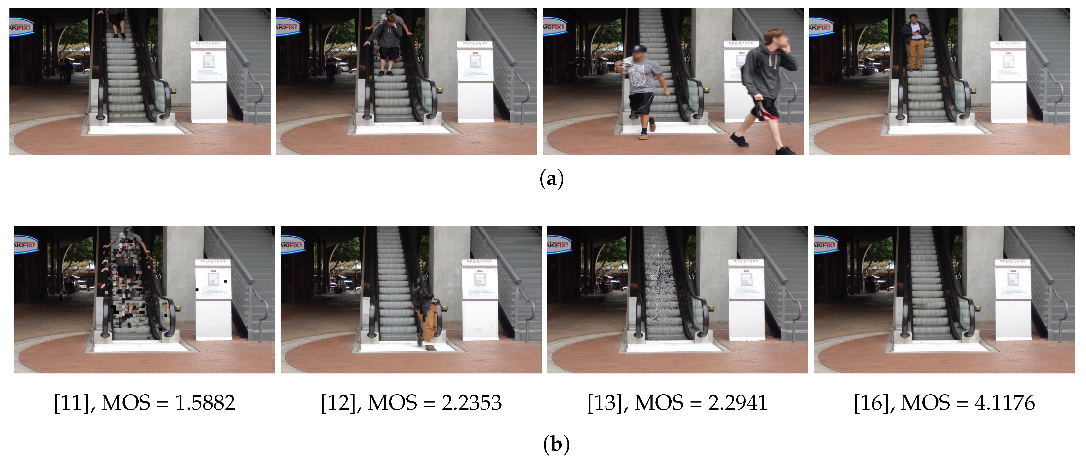
Figure 4 shows an input sequence for a scene in the ReBaQ dataset together with reconstructed background images using different algorithms and corresponding MOS scores. Starting from the leftmost image in Figure 4b, the first image shows an example of a reconstructed background with the presence of a significant amount of foreground residue, which results in a very low subjective score in spite of acceptable perceived image quality in the remaining areas of the scene. The second and the third images have lesser foreground residue as compared to the first and hence are scored higher. The last image has no foreground residue at all and demonstrates good image quality for the most part except for structural deformation in the escalator. This image is scored much higher than all the other three images but still does not get a perfect score.
4. Proposed Reconstructed Background Quality Index
In this section, we propose a full-reference quality index that can automatically assess the perceived quality of the reconstructed background images. The proposed Reconstructed Background Quality Index (RBQI) uses a probability summation model to combine visual characteristics at multiple scales and quantify the deterioration in the perceived quality of the reconstructed background image due to the presence of any residual foreground objects or unnaturalness that may be introduced by the background reconstruction algorithm. The motivation for RBQI comes from the fact that the quality of a reconstructed background image depends on two factors namely:
- (i)
- the visibility of the foreground objects, and
- (ii)
- the visible artifacts introduced while reconstructing the background image.
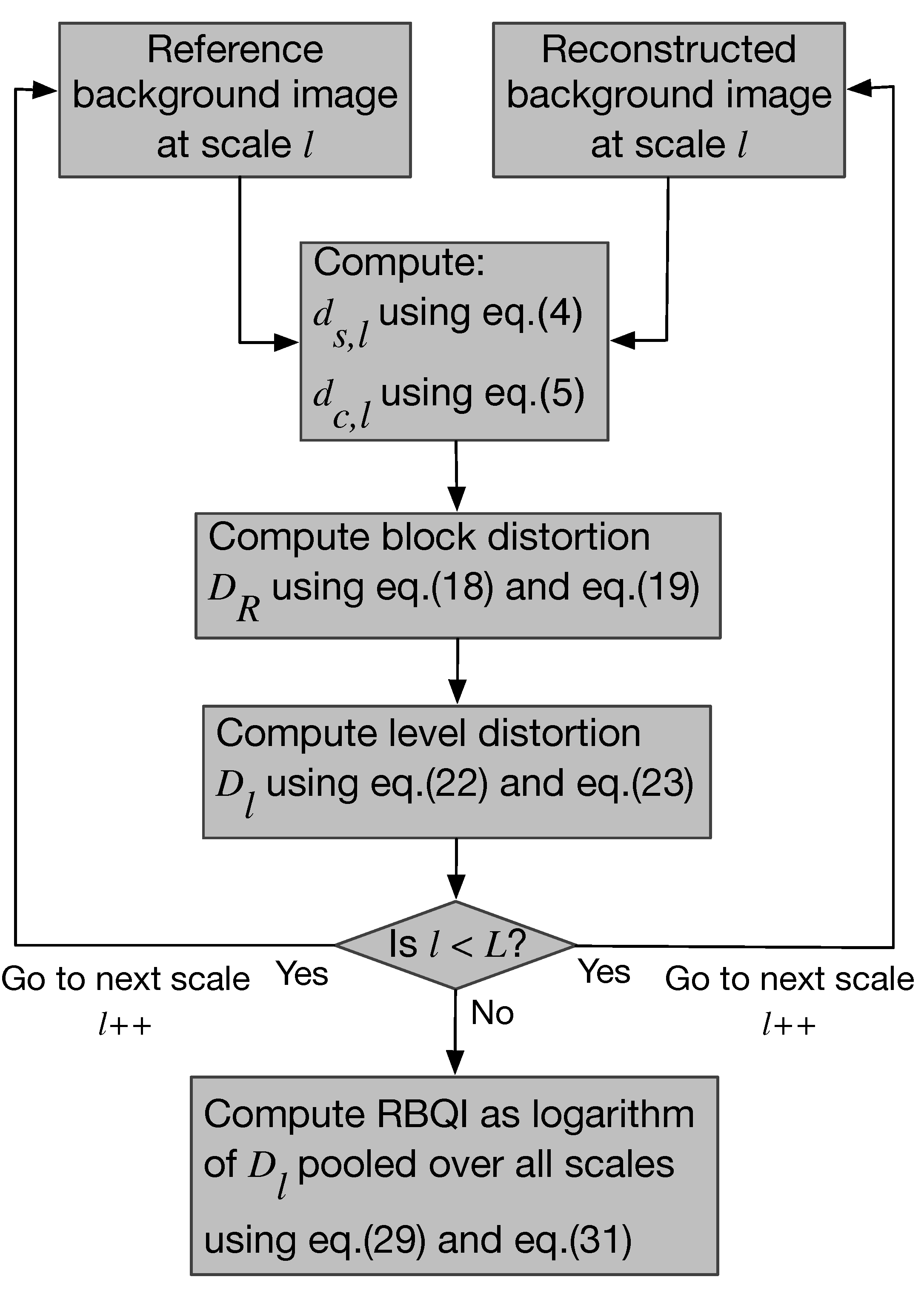
A block diagram of the proposed quality index (RBQI) is shown in Figure 5. An L-level multi-scale decomposition of the reference and reconstructed background images is obtained through lowpass filtering using an averaging filter [19] and downsampling, where corresponds to the finest scale and corresponds to the coarsest scale. For each level , contrast, structure and color differences are computed locally at each pixel to produce a contrast-structure difference map and a color difference map. The difference maps are combined in local regions within each scale and later across scales using a ‘probability summation model’ to predict the perceived quality of the reconstructed background image. More details about the computation of the difference maps and the proposed RBQI based on a probability summation model are provided below.
4.1. Structure Difference Map ()
An image can be decomposed into three different components: luminance, contrast and structure, which are local features computed at every pixel location of the image as described in [29]. By comparing these components, similarity between two images can be calculated [19,29]. A reconstructed background image is formed by mosaicing together parts of different input images. For such an image to appear natural, it is important that the structural continuity be maintained. Preservation of the local luminance from the reference background image is of low relevance as long as this structure continuity is maintained. Any sudden variation in the local luminance across the reconstructed background image manifests itself as contrast or structure deviation from the reference image. Thus, we consider only contrast and structure for comparing the reference and reconstructed background images while leaving out the luminance component. These contrast and structure differences between the reference and the reconstructed background images, calculated at each pixel, give us the ‘contrast-structure similarity map’ referred to as ‘structure map’ for short in the rest of the paper.
First, the structure similarity between the reference and the reconstructed background image, referred to as Structure Index (), is calculated at each pixel location using [29]:
where r is the reference background image, i is the reconstructed background image, and is the cross-correlation between image patches centered at location in the reference and reconstructed background images. and are the standard deviations computed using pixel values in a patch centered at location in the reference and reconstructed background image, respectively. C is a small constant to avoid instability and is calculated as , K is set to and is the maximum possible value of the pixel intensity (255 in this case) [29]. A higher value indicates higher similarity between the pixels in the reference and reconstructed background images.
The background scenes often contain pseudo-stationary objects such as waving trees, escalator, local and global illumination changes. Even though these pseudo-stationary pixels belong to the background, because of the presence of motion, they are likely to be classified as foreground pixels. For this reason, the pseudo-stationary backgrounds pose an additional challenge for the quality assessment algorithms. Just comparing co-located pixel neighborhoods in the two considered images is not sufficient in the presence of such dynamic backgrounds, our algorithm uses a search window of size centered at the current pixel in the reconstructed image, where is an odd value. The is calculated between the pixel at location in the reference image and pixels within the search window centered at pixel in the reconstructed image. The resulting matrix is of size . The modified Equation (1) to calculate for every pixel location in the window centered at is given as:
where
The maximum value of the matrix is taken to be the final value for the pixel at location as given below:
The map takes on values between [−1, 1].
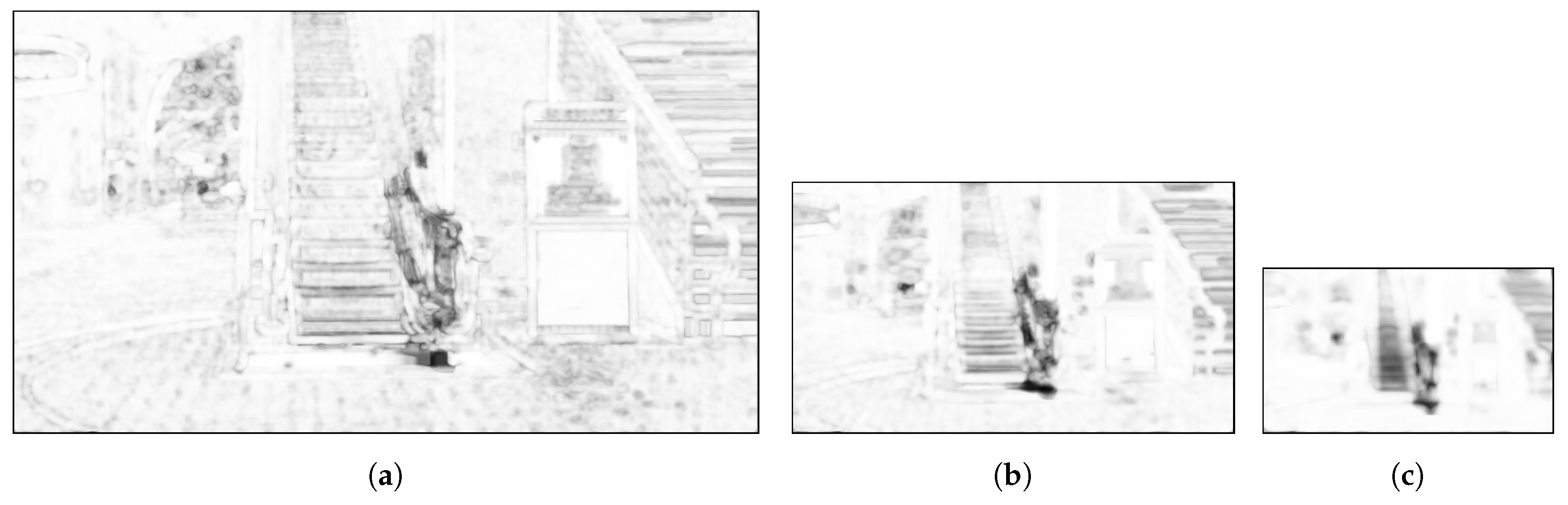
In the proposed method, the map is computed at L different scales denoted as , , . The SI maps generated at three different scales for the background image shown in Figure 4b and reconstructed using the method of [12] are shown in Figure 6. The darker regions in these images indicate larger structure differences between the reference and the reconstructed background images while the lighter regions indicate higher similarities. From Figure 6c, it can also be seen that the computed SI maps show the structure distortions while being robust to the escalator motion in the background.
The structure difference map is calculated using the map at each scale l as follows:
takes on values between [0, 1], where the value of 0 corresponds to no difference while 1 corresponds to the largest difference.
4.2. Color Distance ()
The map is vulnerable to failures while detecting differences in areas of background images with no texture or no structural information. For example, the interior region of a large solid foreground object such as a car does not have much structural information but can differ in color from the background. It should be noted that we use the term “color” here to refer to both luminance and chrominance components. It is important to include the luminance difference while computing the color differences to account for situations where the foreground objects do not vary in color but just in luminance, for example, shadows of foreground objects in the scene. Hence, we incorporate the color information at every scale while calculating the RBQI. The color difference between the filtered reference and reconstructed background images at each scale l is then calculated as the Euclidian distance between the values of co-located pixels in the color space as follows:
4.3. Computation of the Reconstructed Background Quality Index (RBQI) Based on Probability Summation
As indicated previously, the reference and reconstructed background images are decomposed each into a multi-scale pyramid with L levels. Structure difference maps and color difference maps are computed at every level as described in Equations (4) and (5), respectively. These difference maps are pooled together within the scale and later across all scales using a probability summation model [55] to give the final RBQI.
The probability summation model as described in [55] considers an ensemble of independent difference detectors at every pixel location in the image. These detectors predict the probability of perceiving the difference between the reference and the reconstructed background images at the corresponding pixel location based on its neighborhood characteristics in the reference image. Using this model, the probability of the structure difference detector signaling the presence of a structure difference at pixel location at level l can be modeled as an exponential of the form:
where is a parameter chosen to increase the correspondence of RBQI with the experimentally determined MOS scores on a training dataset as described in Section 5.2 and is a parameter whose value depends upon the texture characteristics of the neighborhood centered at in the reference image. The value of is chosen to take into account that differences in structure are less perceptible in textured areas as compared to non-textured areas and that the perception of these differences depends on the scale l.
In order to determine the value of , every pixel in the reference background image at scale l is classified as textured or non-textured using the technique in [56]. This method first calculates the local variance at each pixel using a 3 × 3 window centered around it. Based on the computed variances, a pixel is classified as edge, texture or uniform. By considering the number of edge, texture and uniform pixels in the 8 × 8 neighborhood of the pixel, it is further classified into one of the six types: uniform, uniform/texture, texture, edge/texture, medium edge and strong edge. For our application, we label the pixels classified as ‘texture’ and ‘edge/texture’ as ’textured’ pixels and we label the rest as ‘non-textured’ pixels.
Let be the flag indicating that a pixel is textured. Thus, values of can be expressed as:
when , the value of a should be large enough such that . In our implementation, we chose the value of . Thus, in our current implementation, takes on the form of a binary function that can be replaced with a computationally efficient model obtained by replacing division by in Equation (6) with multiplication by weight . In the remainder of the paper, we keep the notation in Equation (6) to accommodate a more generalized adaptation model based on local image characteristics in textured areas.
Similarly, the probability of the color difference detector signaling the presence of a color difference at pixel location at level l can be modeled as:
where is found in a similar way to and corresponds to the Adaptive Just Noticeable Distortion (AJNCD) calculated at every pixel in the color space as given in [57]:
where and correspond, respectively, to the a and b color values of the pixel located at in the Lab color space, is set to 2.3 [58], and is the mean background luminance of the pixel at and is the maximum luminance gradient across pixel . In Equation (9), is the scaling factor for the chroma components as is given by [57]:
is the scaling factor that simulates the local luminance texture masking and is given by:
where is the weighting factor as described in [57]. Thus, varies at every pixel location based on the distance between the chroma values and texture masking properties of its neighborhood.
A pixel at the l-th level is said to have no distortion if and only if neither the structure difference detector nor the color difference detector at location signal the presence of a difference. Thus, the probability of detecting no difference between the reference and reconstructed background images at pixel and level l can be written as:
A less localized probability of difference detection can be computed by adopting the “probability summation” hypothesis [55], which pools the localized detection probabilities over a region R.
The probability summation hypothesis is based on the following two assumptions:
Assumption 1.
A structure difference is detected in the region of interest R if and only if at least one detector in R signals the presence of a difference, i.e., if and only if at least one of the differences is greater than the threshold and, therefore, considered to be visible. Similarly, a color difference is detected in region R if and only if at least one of the differences is above .
Assumption 2.
The probabilities of detection are independent; i.e., the probability that a particular detector will signal the presence of a difference is independent of the probability that any other detector will. This simplified approximation model is commonly used in the psychophysics literature [55,59] and was found to work well in practice in terms of correlation with human judgement in quantifying perceived visual distortions [60,61].
Then, the probability of no difference detection over the region R is given by:
In the human visual system, the highest visual acuity is limited to the size of the foveal region, which covers approximately of visual angle. In our work, we consider the image regions R as foveal regions approximated by non-overlapping image blocks.
The probability of no distortion detection over the l-th level is obtained by pooling the no detection probabilities over all the regions R in level l and is given by:
or
where
Similarly, we adopt a “probability summation” hypothesis to pool the detection probability across scales. It should be noted that the Human Visual Systems (HVS) dependent parameters and that are included in Equations (14) and (15), respectively, account for the varying sensitivity of the HVS at varying scales. The final probability of detecting no distortion in a reconstructed background image i is obtained when no distortion is detected at any scale and is computed by pooling the no detection probabilities over all scales l, , as follows:
or
where
where and are given by Equations (22) and (23), respectively. From Equations (26) and (27), it can be seen that and take the form of a Minkowski metric with exponent and , respectively.
In Equation (29), and are given by Equations (14) and (15), respectively. Thus, the probability of detecting a difference between the reference image and a reconstructed background image i is given as:
As it can be seen from Equation (30), a lower value of D results in a lower probability of difference detection while a higher value results in a higher probability of difference detection. Therefore, D can be used to assess the perceived quality in the reconstructed background image, with a lower value of D corresponding to a higher perceived quality.
The final Reconstructed Background Quality Index (RBQI) for a reconstructed background image is calculated using the logarithm of D as follows:
As D increases, the value of RBQI increases implying more perceived distortion and thus lower quality of the reconstructed background image. The logarithmic mapping models the saturation effect, i.e., beyond a certain point, the maximum annoyance level is reached and more distortion does not affect the quality.
5. Results
In this section, we analyze the performance of RBQI in terms of its ability to predict the subjective ratings for the perceived quality of reconstructed background images. We evaluate the performance of the proposed quality index in terms of its prediction accuracy, prediction monotonicity and prediction consistency and provide comparisons with the existing statistical and IQA techniques. In our implementation, we set , , . The choice of these parameters is described in more details in Section 5.2. We also evaluate the performance of RBQI for different scales and neighborhood search windows. We conduct a series of hypothesis tests based on the prediction residuals (errors in predictions) after nonlinear regression. These tests help in making statistically meaningful conclusions on the obtained performance results. We also conduct a sensitivity analysis test on the ReBaQ dataset as described in Section 5.3.
We use the two datasets ReBaQ and S-ReBaQ described in Section 3.1 to quantify and compare the performance of RBQI. For evaluating the performance in terms of prediction accuracy, we used the Pearson correlation coefficient (PCC) and root mean squared error (RMSE). The prediction monotonicity is evaluated using the Spearman rank-order correlation coefficient (SROCC). Finally, the Outlier Ratio (OR) (calculated as percentage of the number of of predictions outside the range of times the standard deviations of the MOS scores) is used as a measure of prediction consistency. A 4-parameter regression function [62] is applied to the IQA metrics to provide a nonlinear mapping between the objective scores and the subjective mean opinion scores (MOS):
where denotes the predicted quality for the ith image and denotes the quality score after fitting, and , are the regression model parameters. along with MOS scores are used to calculate the values given in Table 1, Table 2 and Table 3.
5.1. Performance Comparison
Table 1 and Table 2 show the obtained performance evaluation results of the proposed RBQI technique on the ReBaQ and S-ReBaQ datasets, respectively, as compared to the existing statistical and FR-IQA algorithms. The results show that the proposed quality index performs better in terms of prediction accuracy (PCC, RMSE) and prediction consistency (OR) as compared to any other existing technique. In terms of prediction monotonicity (SROCC), the proposed quality index is close in performance to the best performing measure for all datasets except for the ReBaQ-Dynamic dataset. Though the statistical techniques are shown to not correlated well with the subjective scores in terms of PCC on either of the datasets, pCEPs is found to perform marginally better in terms of SROCC as compared to RBQI. Among the FR-IQA algorithms, the performance of the NQM [34] comes close to the proposed technique for scenes with static background images, i.e., for the ReBaQ-Static dataset, as it considers the effects of contrast sensitivity, luminance variations, contrast interaction between spatial frequencies and contrast masking effect while weighting the SNR between the ground truth and reconstructed image. The more popular MS-SSIM [19] technique is shown to not correlate well with the subjective scores for the ReBaQ dataset. This is because the MS-SSIM calculates the final quality index of the image by just averaging over the entire image. In the problem of background reconstruction, the error might occupy a relatively small area as compared to the image size, thereby under-penalizing the residual foreground. Most of the existing FR-IQA techniques perform poorly for the ReBaQ-Dynamic dataset. This is because the assumption of pixel-to-pixel correspondence is no longer valid in the presence of pseudo-stationary background. The proposed RBQI technique uses a neighborhood window to handle such backgrounds, thereby improving the performance over NQM [34] by a margin of 10% and by 30% over MS-SSIM [19]. Additionally, as shown in Table 3, the proposed RBQI technique is found to perform significantly better in terms of PCC, RMSE and OR as compared to any of the existing IQA techniques on the larger dataset formed by combining the ReBaQ and S-ReBaQ datasets. Though RBQI is second best in terms of SROCC, it closely follows the best performing measure (pCEPs) for the combined dataset. CQM [20], which is used in the Scene Background Modeling Challenge 2016 (SBMC) [21,22] to compare the performance of the algorithms, performs poorly on the combined dataset and hence is not a good choice for evaluating the quality of reconstructed background images and not suitable for comparing the performance of background reconstruction algorithms.
The P-value is the probability of getting a correlation as large as the observed value by random chance. If the P-value is less than 0.05, then the correlation is significant. The P-values (P and P) reported in Table 1, Table 2 and Table 3 indicate that most of the correlation scores are statistically significant.
5.2. Model Parameter Selection
The proposed quality index accepts four parameters:
In Table 4, we evaluate our algorithm with different values for the parameters. These simulations were run only on the ReBaQ dataset. Table 4a shows the effect of varying values on the performance of RBQI. The performance of RBQI for ReBaQ improved slightly with the increase in the neighborhood search window size as expected, but the performance of RBQI increased drastically for the ReBaQ dataset from to before starting to drop at . Thus, we chose for all our experiments. Table 4b gives performance results for a different number of scales. As a trade-off between the computation complexity and prediction accuracy, we chose the number of scales to be . The probability summation model parameters and were found such that they maximized the correlation between RBQI and MOS scores on the ReBaQ dataset. As in [63], we divided the ReBaQ dataset into two subsets by randomly choosing 80% of the total images for training and 20% for testing. The random training-testing procedure was repeated 100 times and the parameters were averaged over the 100 iterations. Values were found to correlate well with the subjective test scores.
5.3. Sensitivity Analysis
In addition to the statistical significance tests, we conduct sensitivity tests on the ReBaQ dataset by generating multiple smaller datasets and comparing the performance of the different techniques on these smaller datasets. These experiments were carried out on the ReBaQ-Static and ReBaQ-Dynamic datasets separately. For this purpose, we create 1000 smaller datasets from the ReBaQ-Static by randomly sampling n images such that n is smaller than the size of the dataset and such that the corresponding MOS scores cover the entire scoring range. For every dataset of size n, we calculate the PCC values after applying the nonlinear mapping of Equation (32). The mean and the standard deviation of the PCC scores, denoted by and respectively, over the 1000 datasets are calculated for and and are given in Table 5. Similar sensitivity tests were conducted on the ReBaQ-Dynamic dataset to obtain the values in Table 5. As it can be seen from Table 5, the standard deviations of the PCC across 1000 datasets of size n are very small and the relative rank of the different techniques is maintained as in Table 1.
6. Conclusions
In this paper, we addressed the problem of quality evaluation of reconstructed background images. We first proposed two different datasets for benchmarking the performance of existing and future techniques proposed to evaluate the quality of reconstructed background images. Then, we proposed the first full-reference Reconstructed Background Quality Index (RBQI) to objectively measure the perceived quality of the reconstructed background images.
The RBQI uses the probability summation model to combine visual characteristics at multiple scales and to quantify the deterioration in the perceived quality of the reconstructed background image due to the presence of any foreground objects or unnaturalness that may be introduced by the background reconstruction algorithm. The use of a neighborhood search window while calculating the contrast and structure differences provides further boost in the performance in the presence of pseudo-stationary background while not affecting the performance on scenes with static background. The probability summation model penalizes only the perceived differences across the reference and reconstructed background images while the unperceived differences do not affect the RBQI, thereby giving better correlation with the subjective scores. Experimental results on the benchmarking datasets showed that the proposed measure out-performed existing statistical and IQA techniques in estimating the perceived quality of reconstructed background images.
The proposed RBQI has multiple applications. It can be used by the algorithm developers to optimize the performance of their techniques by users to compare different background reconstruction algorithms and to determine which algorithm is best suited for their task. It can also be deployed in challenges (e.g., SBMC [22]) that promote the development of improved background reconstruction algorithms. As future work, the authors will investigate the development of a no-reference quality index for assessing the perceived quality of reconstructed background images in scenarios where the reference background images are not available. The no-reference metric can also be used as a feedback to the algorithm to adaptively optimize its performance.
Supplementary Materials
The ReBaQ and S-ReBaQ datasets and source code for RBQI will be available for download at the authors’ website https://github.com/ashrotre/RBQI or https://ivulab.asu.edu.
Author Contributions
A.S. and L.J.K. contributed to the design and development of the proposed method and to the writing of the manuscript. A.S. contributed additionally to the software implementation and testing of the proposed method.
Funding
This research received no external funding.
Conflicts of Interest
The authors declare no conflict of interest.
Abbreviations
The following abbreviations are used in this manuscript:
| RBQI | Reconstructed Background Quality Index |
| PSNR | Peak Signal to Noise Ratio |
| AGE | Average Gray-level Error |
| EPs | Number of Error Pixels |
| pEPs | percentage of Error Pixels |
| CEPs | number of Clustered Error Pixels |
| pCEPs | percentage of Clustered Error Pixels |
| IQA | Image Quality Analysis |
| FR-IQA | Full Reference Image Quality Assessment |
| HVS | Human Visual System |
| MS-SSIM | Multi-scale Structural SIMilarity index |
| CQM | Color image Quality Measures |
| PETS | Performance Evaluation of Tracking and Surveillance |
| SBMNet | Scene Background Modeling Net |
| SSIM | Structural SIMilarity index |
| VSNR | Visual Signal to Noise ratio |
| VIF | Visual Information Fidelity |
| VIFP | pixel-based Visual Information Fidelity |
| UQI | Universal Quality Index |
| IFC | Image Fidelity Criterion |
| NQM | Noise Quality Measure |
| WSNR | Weights Signal to Noise Ratio |
| FSIM | Feature SIMilarity index |
| FSIMc | Feature SIMilarity index with color |
| SR-SIM | Spectral Residual SIMilarity index |
| SalSSIM | Saliency-based Structural SIMilarity index |
| ReBaQ | Reconstructed Background Quality dataset |
| S-ReBaQ | SBMNet based Reconstructed Background Quality dataset |
| SBMC | Scene Background Modeling |
| MOS | Mean Opinion Score |
| PCC | Pearson Correlation Coefficient |
| SROCC | Spearman Rank Order Correlation Coefficient |
| RMSE | Root Mean Square Error |
| OR | Outlier Ratio |
References
- Colque, R.M.; Cámara-Chávez, G. Progressive Background Image Generation of Surveillance Traffic Videos Based on a Temporal Histogram Ruled by a Reward/Penalty Function. In Proceedings of the 2011 24th SIBGRAPI Conference on Graphics, Patterns and Images (Sibgrapi), Maceio, Brazil, 28–31 August 2011; pp. 297–304. [Google Scholar]
- Stauffer, C.; Grimson, W.E.L. Learning patterns of activity using real-time tracking. IEEE Trans. Pattern Anal. Mach. Intell. 2000, 22, 747–757. [Google Scholar] [CrossRef] [Green Version]
- Li, L.; Huang, W.; Gu, I.Y.H.; Tian, Q. Statistical modeling of complex backgrounds for foreground object detection. IEEE Trans. Image Process. 2004, 13, 1459–1472. [Google Scholar] [CrossRef] [PubMed]
- Fleuret, F.; Berclaz, J.; Lengagne, R.; Fua, P. Multicamera People Tracking with a Probabilistic Occupancy Map. IEEE Trans. Pattern Anal. Mach. Intell. 2008, 30, 267–282. [Google Scholar] [CrossRef] [PubMed] [Green Version]
- Flores, A.; Belongie, S. Removing pedestrians from google street view images. In Proceedings of the IEEE Computer Society Conference on Computer Vision and Pattern Recognition Workshops, San Francisco, CA, USA, 13–18 June 2010; pp. 53–58. [Google Scholar]
- Jones, W.D. Microsoft and Google vie for virtual world domination. IEEE Spectr. 2006, 43, 16–18. [Google Scholar] [CrossRef]
- Zheng, E.; Chen, Q.; Yang, X.; Liu, Y. Robust 3D modeling from silhouette cues. In Proceedings of the IEEE International Conference on Acoustics, Speech and Signal Processing, Taipei, Taiwan, 19–24 April 2009; pp. 1265–1268. [Google Scholar]
- Maddalena, L.; Petrosino, A. A Self-Organizing Approach to Background Subtraction for Visual Surveillance Applications. IEEE Trans. Image Process. 2008, 17, 1168–1177. [Google Scholar] [CrossRef] [PubMed] [Green Version]
- Varadarajan, S.; Karam, L.; Florencio, D. Background subtraction using spatio-temporal continuities. In Proceedings of the 2010 2nd European Workshop on Visual Information Processing, Paris, France, 5–6 July 2010; pp. 144–148. [Google Scholar]
- Farin, D.; de With, P.; Effelsberg, W. Robust background estimation for complex video sequences. In Proceedings of the IEEE International Conference on Image Processing, Barcelona, Spain, 14–17 September 2003; Volume 1, pp. 145–148. [Google Scholar]
- Hsiao, H.H.; Leou, J.J. Background initialization and foreground segmentation for bootstrapping video sequences. EURASIP J. Image Video Process. 2013, 1, 12. [Google Scholar] [CrossRef]
- Reddy, V.; Sanderson, C.; Lovell, B. A low-complexity algorithm for static background estimation from cluttered image sequences in surveillance contexts. EURASIP J. Image Video Process. 2010, 1, 1:1–1:14. [Google Scholar] [CrossRef]
- Yao, J.; Odobez, J. Multi-Layer Background Subtraction Based on Color and Texture. In Proceedings of the IEEE Conference on Computer Vision and Pattern Recognition, Minneapolis, MN, USA, 17–22 June 2007; pp. 1–8. [Google Scholar]
- Colombari, A.; Fusiello, A. Patch-Based Background Initialization in Heavily Cluttered Video. IEEE Trans. Image Process. 2010, 19, 926–933. [Google Scholar] [CrossRef] [PubMed] [Green Version]
- Herley, C. Automatic occlusion removal from minimum number of images. In Proceedings of the IEEE International Conference on Image Processing, Genova, Italy, 14 September 2005; Volume 2, pp. 1046–1049. [Google Scholar]
- Agarwala, A.; Dontcheva, M.; Agrawala, M.; Drucker, S.; Colburn, A.; Curless, B.; Salesin, D.; Cohen, M. Interactive Digital Photomontage. ACM Trans. Gr. 2004, 23, 294–302. [Google Scholar] [CrossRef]
- Shrotre, A.; Karam, L. Background recovery from multiple images. In Proceedings of the IEEE Digital Signal Processing and Signal Processing Education Meeting, Napa, CA, USA, 11–14 August 2013; pp. 135–140. [Google Scholar]
- Maddalena, L.; Petrosino, A. Towards Benchmarking Scene Background Initialization. In 2015 ICIAP: New Trends in Image Analysis and Processing—ICIAP 2015 Workshops; Springer: Berlin, Germany, 2015; pp. 469–476. [Google Scholar]
- Wang, Z.; Simoncelli, E.; Bovik, A. Multiscale structural similarity for image quality assessment. In Proceedings of the Asilomar Conference on Signals, Systems and Computers, Pacific Grove, CA, USA, 9–12 November 2003; Volume 2, pp. 1398–1402. [Google Scholar]
- Yalman, Y.; Ertürk, İ. A new color image quality measure based on YUV transformation and PSNR for human vision system. Turk. J. Electr. Eng. Comput. Sci. 2013, 21, 603–612. [Google Scholar]
- Bouwmans, T.; Maddalena, L.; Petrosino, A. Scene background initialization: A taxonomy. Pattern Recognit. Lett. 2017, 96, 3–11. [Google Scholar] [CrossRef]
- Maddalena, L.; Jodoin, P. Scene Background Modeling Contest (SBMC2016). Available online: http://www.icpr2016.org/site/session/scene-background-modeling-sbmc2016/ (accessed on 15 May 2018).
- Toyama, K.; Krumm, J.; Brumitt, B.; Meyers, B. Wallflower: principles and practice of background maintenance. In Proceedings of the IEEE International Conference on Computer Vision, Kerkyra, Greece, 20–27 September 1999; Volume 1, pp. 255–261. [Google Scholar]
- Mahadevan, V.; Vasconcelos, N. Spatiotemporal Saliency in Dynamic Scenes. IEEE Trans. Pattern Anal. Mach. Intell. 2010, 32, 171–177. [Google Scholar] [CrossRef] [PubMed]
- Sheikh, Y.; Shah, M. Bayesian modeling of dynamic scenes for object detection. IEEE Trans. Pattern Anal. Mach. Intell. 2005, 27, 1778–1792. [Google Scholar] [CrossRef] [PubMed] [Green Version]
- Jodoin, P.; Maddalena, L.; Petrosino, A. SceneBackgroundModeling.Net (SBMnet). Available online: www.SceneBackgroundModeling.net (accessed on 15 May 2018).
- Jodoin, P.M.; Maddalena, L.; Petrosino, A.; Wang, Y. Extensive Benchmark and Survey of Modeling Methods for Scene Background Initialization. IEEE Trans. Image Process. 2017, 26, 5244–5256. [Google Scholar] [CrossRef] [PubMed]
- Shrotre, A.; Karam, L. Visual quality assessment of reconstructed background images. In Proceedings of the International Conference on Quality of Multimedia Experience, Lisbon, Portugal, 6–8 June 2016; pp. 1–6. [Google Scholar]
- Wang, Z.; Bovik, A.; Sheikh, H.; Simoncelli, E. Image quality assessment: From error visibility to structural similarity. IEEE Trans. Image Process. 2004, 13, 600–612. [Google Scholar] [CrossRef] [PubMed]
- Chandler, D.; Hemami, S. VSNR: A Wavelet-Based Visual Signal to Noise Ratio for Natural Images. IEEE Trans. Image Process. 2007, 16, 2284–2298. [Google Scholar] [CrossRef] [PubMed]
- Sheikh, H.; Bovik, A. Image information and visual quality. IEEE Trans. Image Process. 2006, 15, 430–444. [Google Scholar] [CrossRef] [PubMed] [Green Version]
- Wang, Z.; Bovik, A. A universal image quality index. IEEE Sign. Process. Lett. 2002, 9, 81–84. [Google Scholar] [CrossRef]
- Sheikh, H.; Bovik, A.; de Veciana, G. An information fidelity criterion for image quality assessment using natural scene statistics. IEEE Trans. Image Process. 2005, 14, 2117–2128. [Google Scholar] [CrossRef] [PubMed] [Green Version]
- Damera-Venkata, N.; Kite, T.; Geisler, W.; Evans, B.; Bovik, A. Image quality assessment based on a degradation model. IEEE Trans. Image Process. 2000, 9, 636–650. [Google Scholar] [CrossRef] [PubMed]
- Mitsa, T.; Varkur, K. Evaluation of contrast sensitivity functions for the formulation of quality measures incorporated in halftoning algorithms. In Proceedings of the IEEE International Conference on Acoustics Speech, and Signal Processing, Minneapolis, MN, USA, 27–30 April 1993; Volume 5, pp. 301–304. [Google Scholar]
- Zhang, L.; Zhang, D.; Mo, X.; Zhang, D. FSIM: A Feature Similarity Index for Image Quality Assessment. IEEE Trans. Image Process. 2011, 20, 2378–2386. [Google Scholar] [CrossRef] [PubMed] [Green Version]
- Zhang, L.; Li, H. SR-SIM: A fast and high performance IQA index based on spectral residual. In Proceedings of the 2012 19th IEEE International Conference on Image Processing, Orlando, FL, USA, 30 September–3 October 2012; pp. 1473–1476. [Google Scholar]
- Akamine, W.; Farias, M. Incorporating visual attention models into video quality metrics. In Proceedings of SPIE; SPIE: Bellingham, WA, USA, 2014; Volume 9016, pp. 1–9. [Google Scholar]
- Lin, W.; Kuo, J.C.C. Perceptual visual quality metrics: A survey. J. Vis. Commun. Image Represent. 2011, 22, 297–312. [Google Scholar] [CrossRef] [Green Version]
- Chandler, D.M. Seven Challenges in Image Quality Assessment: Past, Present, and Future Research. ISRN Signal Process. 2013, 1–53. [Google Scholar] [CrossRef]
- Seshadrinathan, K.; Pappas, T.N.; Safranek, R.J.; Chen, J.; Wang, Z.; Sheikh, H.R.; Bovik, A.C. Image Quality Assessment. In The Essential Guide to Image Processing; Bovik, A.C., Ed.; Elsevier: New York, NY, USA, 2009; Chapter 21; pp. 553–595. [Google Scholar] [Green Version]
- Laugraud, B.; Piérard, S.; Van Droogenbroeck, M. LaBGen-P: A pixel-level stationary background generation method based on LaBGen. In Proceedings of the 2016 23rd International Conference on Pattern Recognition, Cancun, Mexico, 4–8 December 2016; pp. 107–113. [Google Scholar]
- Maddalena, L.; Petrosino, A. Extracting a background image by a multi-modal scene background model. In Proceedings of the 2016 23rd International Conference on Pattern Recognition, Cancun, Mexico, 4–8 December 2016; pp. 143–148. [Google Scholar]
- Javed, S.; Jung, S.K.; Mahmood, A.; Bouwmans, T. Motion-Aware Graph Regularized RPCA for background modeling of complex scenes. In Proceedings of the 2016 23rd International Conference on Pattern Recognition, Cancun, Mexico, 4–8 December 2016; pp. 120–125. [Google Scholar]
- Liu, W.; Cai, Y.; Zhang, M.; Li, H.; Gu, H. Scene background estimation based on temporal median filter with Gaussian filtering. In Proceedings of the 2016 23rd International Conference on Pattern Recognition, Cancun, Mexico, 4–8 December 2016; pp. 132–136. [Google Scholar]
- Ramirez-Alonso, G.; Ramirez-Quintana, J.A.; Chacon-Murguia, M.I. Temporal weighted learning model for background estimation with an automatic re-initialization stage and adaptive parameters update. Pattern Recognit. Lett. 2017, 96, 34–44. [Google Scholar] [CrossRef]
- Minematsu, T.; Shimada, A.; Taniguchi, R.I. Background initialization based on bidirectional analysis and consensus voting. In Proceedings of the 2016 23rd International Conference on Pattern Recognition, Cancun, Mexico, 4–8 December 2016; pp. 126–131. [Google Scholar]
- Piccardi, M. Background subtraction techniques: A review. In Proceedings of the IEEE International Conference on Systems, Man and Cybernetics, The Hague, The Netherlands, 10–13 October 2004; Volume 4, pp. 3099–3104. [Google Scholar]
- Halfaoui, I.; Bouzaraa, F.; Urfalioglu, O. CNN-based initial background estimation. In Proceedings of the 2016 23rd International Conference on Pattern Recognition, Cancun, Mexico, 4–8 December 2016; pp. 101–106. [Google Scholar]
- Chacon-Murguia, M.I.; Ramirez-Quintana, J.A.; Ramirez-Alonso, G. Evaluation of the background modeling method Auto-Adaptive Parallel Neural Network Architecture in the SBMnet dataset. In Proceedings of the 2016 23rd International Conference on Pattern Recognition, Cancun, Mexico, 4–8 December 2016; pp. 137–142. [Google Scholar]
- Ortego, D.; SanMiguel, J.C.; Martínez, J.M. Rejection based multipath reconstruction for background estimation in SBMnet 2016 dataset. In Proceedings of the 2016 23rd International Conference on Pattern Recognition, Cancun, Mexico, 4–8 December 2016; pp. 114–119. [Google Scholar]
- Methodology for the Subjective Assessment of the Quality of Television Pictures; Technical Report ITU-R BT.500-13; International Telecommunications Union: Geneva, Switzerland, 2012.
- Snellen, H. Probebuchstaben zur Bestimmung der Sehschärfe; P.W. Van de Weijer: Utrecht, The Netherlands, 1862. [Google Scholar]
- Waggoner, T.L. PseudoIsochromatic Plate (PIP) Color Vision Test 24 Plate Edition. Available online: http://colorvisiontesting.com/ishihara.htm (accessed on 15 May 2018).
- Robson, J.; Graham, N. Probability summation and regional variation in contrast sensitivity across the visual field. Vis. Res. 1981, 21, 409–418. [Google Scholar] [CrossRef]
- Su, J.; Mersereau, R. Post-procesing for artifact reduction in JPEG-compressed images. In Proceedings of the IEEE International Conference on Acoustics, Speech, and Signal Processing, Detroit, MI, USA, 9–12 May 1995; pp. 2363–2366. [Google Scholar]
- Chou, C.H.; Liu, K.C. Colour image compression based on the measure of just noticeable colour difference. IET Image Process. 2008, 2, 304–322. [Google Scholar] [CrossRef]
- Mahy, M.; Eycken, L.; Oosterlinck, A. Evaluation of uniform color spaces developed after the adoption of CIELAB and CIELUV. Color Res. Appl. 1994, 19, 105–121. [Google Scholar]
- Watson, A.; Kreslake, L. Measurement of visual impairment scales for digital video. In Human Vision and Electronic Imaging VI; International Society for Optics and Photonics: Bellingham, WA, USA, 2001; Volume 4299, pp. 79–89. [Google Scholar]
- Watson, A.B. DCT quantization matrices visually optimized for individual images. In Human Vision and Electronic Imaging VI; International Society for Optics and Photonics: Bellingham, WA, USA, 1993; Volume 1913, pp. 202–216. [Google Scholar]
- Hontsch, I.; Karam, L.J. Adaptive image coding with perceptual distortion control. IEEE Trans. Image Process. 2002, 11, 213–222. [Google Scholar] [CrossRef] [PubMed] [Green Version]
- VQEG. Final Report from the Video Quality Experts Group on the Validation of Objective Models of Video Quality Assessment. 2003. Available online: ftp://vqeg.its.bldrdoc.gov/Documents/VQEGApprovedFinalReports/VQEGIIFinalReport.pdf (accessed on 15 May 2018).
- Mittal, A.; Moorthy, A.; Bovik, A. No-Reference Image Quality Assessment in the Spatial Domain. IEEE Trans. Image Process. 2012, 21, 4695–4708. [Google Scholar] [CrossRef] [PubMed] [Green Version]
Figure 1.
Reference background images for different scenes in the Reconstructed Background Quality (ReBaQ) Dataset. Each reference background image corresponds to a captured scene background without foreground objects. (a) Scenes with static backgrounds from the ReBaQ dataset; (b) Scenes with pseudo-stationary backgrounds from the ReBaQ dataset.

Figure 2.
Reference background images for different scenes in the SBMNet based Reconstructed Background Quality (S-ReBaQ) Dataset. Each reference background image corresponds to a captured scene background without foreground objects.
Figure 2.
Reference background images for different scenes in the SBMNet based Reconstructed Background Quality (S-ReBaQ) Dataset. Each reference background image corresponds to a captured scene background without foreground objects.

Figure 3.
Subjective test Graphical User Interface (GUI).

Figure 4.
Example input sequence and recovered background images with corresponding MOS scores from the ReBaQ dataset. (a) Four out of eight input images from the input sequence “Escalator”; (b) Background images reconstructed by different algorithms and corresponding MOS scores.
Figure 4.
Example input sequence and recovered background images with corresponding MOS scores from the ReBaQ dataset. (a) Four out of eight input images from the input sequence “Escalator”; (b) Background images reconstructed by different algorithms and corresponding MOS scores.

Figure 5.
Block diagram describing the computation of the proposed Reconstructed Background Quality Index (RBQI).
Figure 5.
Block diagram describing the computation of the proposed Reconstructed Background Quality Index (RBQI).

Figure 6.
Structure Index (SI) map with for the background image reconstructed using the method in [12] as shown in Figure 4b. The darker regions indicate larger structure differences between the reference and the reconstructed background image. (a) Scale l = 0; (b) Scale l = 1; (c) Scale l = 2.


Table 1.
Comparison of RBQI vs. Statistical measures and IQA techniques on the ReBaQ dataset.
| a. Comparison on the ReBaQ-Static Dataset. | |||||||
| ReBaQ-Static | |||||||
| PCC | SROCC | RMSE | OR | PPCC | PSROCC | ||
| Statistical Measures | AGE | 0.7776 | 0.6348 | 0.6050 | 9.72% | 0.000000 | 0.000000 |
| EPs | 0.3976 | 0.5093 | 0.8829 | 13.89% | 0.000000 | 0.000000 | |
| pEPs | 0.8058 | 0.6170 | 0.5698 | 6.94% | 0.000000 | 0.000000 | |
| CEPs | 0.5719 | 0.6939 | 0.7893 | 11.11% | 0.000000 | 0.000000 | |
| pCEPs | 0.6281 | 0.7843 | 0.9622 | 13.89% | 0.000000 | 0.000000 | |
| Image Quality Assessment Metrics | PSNR | 0.8324 | 0.7040 | 0.5331 | 8.33% | 0.000000 | 0.000000 |
| SSIM [29] | 0.5914 | 0.5168 | 0.7759 | 11.11% | 0.000000 | 0.000177 | |
| MS-SSIM [19] | 0.7230 | 0.7085 | 0.6648 | 8.33% | 0.000000 | 0.000000 | |
| VSNR [30] | 0.5216 | 0.3986 | 0.8209 | 9.72% | 0.000003 | 0.000531 | |
| VIF [31] | 0.3625 | 0.0843 | 0.8968 | 15.28% | 0.001754 | 0.484429 | |
| VIFP [31] | 0.5122 | 0.3684 | 0.8265 | 11.11% | 0.000004 | 0.001470 | |
| UQI [32] | 0.6197 | 0.7581 | 0.9622 | 13.89% | 0.000000 | 0.000000 | |
| IFC [33] | 0.5003 | 0.3771 | 0.8331 | 11.11% | 0.000008 | 0.001105 | |
| NQM [34] | 0.8251 | 0.8602 | 0.5437 | 6.94% | 0.000000 | 0.000000 | |
| WSNR [35] | 0.8013 | 0.7389 | 0.5756 | 5.56% | 0.000000 | 0.000000 | |
| FSIM [36] | 0.7209 | 0.6970 | 0.6668 | 9.72% | 0.000000 | 0.000000 | |
| FSIMc [36] | 0.7274 | 0.7033 | 0.6603 | 9.72% | 0.000000 | 0.000000 | |
| SRSIM [37] | 0.7906 | 0.7862 | 0.5892 | 8.33% | 0.000000 | 0.000000 | |
| SalSSIM [38] | 0.5983 | 0.5217 | 0.7710 | 9.72% | 0.000000 | 0.000003 | |
| CQM [20] | 0.6401 | 0.5755 | 0.7393 | 8.33% | 0.000000 | 0.000000 | |
| RBQI(Proposed) | 0.9006 | 0.8592 | 0.4183 | 4.17% | 0.000000 | 0.000000 | |
| b. Comparison on the ReBaQ-Dynamic Dataset. | |||||||
| ReBaQ-Dynamic | |||||||
| PCC | SROCC | RMSE | OR | PPCC | PSROCC | ||
| Statistical Measures | AGE | 0.4999 | 0.2303 | 0.7644 | 9.72% | 0.005000 | 0.051600 |
| EPs | 0.1208 | 0.2771 | 0.8761 | 13.89% | 0.007600 | 0.018500 | |
| pEPs | 0.4734 | 0.2771 | 0.8825 | 9.72% | 0.007600 | 0.018500 | |
| CEPs | 0.5951 | 0.7549 | 0.7092 | 11.11% | 0.000000 | 0.000000 | |
| pCEPs | 0.6418 | 0.7940 | 0.8826 | 15.28% | 0.000000 | 0.000000 | |
| Image Quality Assessment Metrics | PSNR | 0.5133 | 0.4179 | 0.7575 | 8.33% | 0.000004 | 0.000263 |
| SSIM [29] | 0.0135 | 0.0264 | 0.8826 | 15.28% | 0.910238 | 0.822439 | |
| MS-SSIM [19] | 0.5087 | 0.4466 | 0.7598 | 9.72% | 0.000005 | 0.000085 | |
| VSNR [30] | 0.5090 | 0.1538 | 0.7597 | 9.72% | 0.000005 | 0.198310 | |
| VIF [31] | 0.3103 | 0.3328 | 0.8390 | 13.89% | 0.199921 | 0.236522 | |
| VIFP [31] | 0.4864 | 0.1004 | 0.7711 | 9.72% | 0.000015 | 0.403684 | |
| UQI [32] | 0.6262 | 0.7450 | 0.8826 | 15.28% | 0.000000 | 0.000000 | |
| IFC [33] | 0.4306 | 0.1024 | 0.7966 | 11.11% | 0.000160 | 0.394409 | |
| NQM [34] | 0.6898 | 0.6600 | 0.6390 | 9.72% | 0.000000 | 0.000000 | |
| WSNR [35] | 0.6409 | 0.5760 | 0.6775 | 9.72% | 0.000000 | 0.000000 | |
| FSIM [36] | 0.5131 | 0.3283 | 0.7575 | 9.72% | 0.000004 | 0.004922 | |
| FSIMc [36] | 0.5144 | 0.3310 | 0.7568 | 9.72% | 0.000004 | 0.004559 | |
| SRSIM [37] | 0.5512 | 0.5376 | 0.7364 | 11.11% | 0.000001 | 0.000001 | |
| SalSSIM [38] | 0.4866 | 0.3200 | 0.7710 | 9.72% | 0.000015 | 0.006198 | |
| CQM [20] | 0.7050 | 0.7610 | 0.6259 | 8.33% | 0.000000 | 0.000000 | |
| RBQI(Proposed) | 0.7908 | 0.6773 | 0.5402 | 5.56% | 0.000000 | 0.000000 | |
Table 2.
Comparison of RBQI vs. Statistical measures and IQA techniques on the S-ReBaQ dataset.
| S-ReBaQ | |||||||
|---|---|---|---|---|---|---|---|
| PCC | SROCC | RMSE | OR | PPCC | PSROCC | ||
| Statistical Measures | AGE | 0.6453 | 0.6238 | 2.2373 | 14.84% | 0.392900 | 0.000000 |
| EPs | 0.4202 | 0.1426 | 1.2049 | 24.73% | 0.000000 | 0.000000 | |
| pEPs | 0.0505 | 0.4990 | 1.6676 | 26.92% | 0.498331 | 0.000000 | |
| CEPs | 0.6283 | 0.6666 | 0.8491 | 18.68% | 0.000000 | 0.000000 | |
| pCEPs | 0.8346 | 0.8380 | 0.6011 | 6.59% | 0.000000 | 0.000000 | |
| Image Quality Assessment Metrics | PSNR | 0.7099 | 0.6834 | 0.7686 | 6.59% | 0.000000 | 0.000000 |
| SSIM [29] | 0.5975 | 0.5827 | 0.8751 | 12.09% | 0.000000 | 0.000000 | |
| MS-SSIM [19] | 0.8048 | 0.8030 | 0.6478 | 29.12% | 0.000000 | 0.000000 | |
| VSNR [30] | 0.0850 | 0.1717 | 1.0874 | 13.19% | 0.253675 | 0.486686 | |
| VIF [31] | 0.1027 | 0.2064 | 1.0914 | 27.47% | 0.167842 | 0.005305 | |
| VIFP [31] | 0.6081 | 0.6240 | 0.8664 | 26.92% | 0.000000 | 0.000000 | |
| UQI [32] | 0.6316 | 0.5932 | 0.8461 | 14.84% | 0.000000 | 0.000000 | |
| IFC [33] | 0.6235 | 0.6020 | 0.8533 | 16.48% | 0.000000 | 0.000000 | |
| NQM [34] | 0.7950 | 0.7816 | 0.6621 | 14.84% | 0.000000 | 0.000000 | |
| WSNR [35] | 0.7176 | 0.6888 | 0.7601 | 7.14% | 0.000000 | 0.000000 | |
| FSIM [36] | 0.7243 | 0.7157 | 0.7525 | 10.44% | 0.000000 | 0.000000 | |
| FSIMc [36] | 0.7278 | 0.7172 | 0.7484 | 12.09% | 0.000000 | 0.000000 | |
| SRSIM [37] | 0.7853 | 0.7538 | 0.6757 | 12.09% | 0.000000 | 0.000000 | |
| SalSSIM [38] | 0.7356 | 0.7300 | 0.7393 | 7.14% | 0.000000 | 0.000000 | |
| CQM [20] | 0.2634 | 0.3645 | 1.0531 | 8.24% | 0.000327 | 0.000276 | |
| RBQI(Proposed) | 0.8613 | 0.8222 | 0.5545 | 3.30% | 0.000000 | 0.000000 | |
Table 3.
Comparison of RBQI vs. Statistical measures and IQA techniques on a combined ReBaQ and S-ReBaQ dataset.
Table 3.
Comparison of RBQI vs. Statistical measures and IQA techniques on a combined ReBaQ and S-ReBaQ dataset.
| ReBaQ and S-ReBaQ Combined | |||||||
|---|---|---|---|---|---|---|---|
| PCC | SROCC | RMSE | OR | PPCC | PSROCC | ||
| Statistical Measures | AGE | 0.6667 | 0.6593 | 0.8462 | 14.42% | 0.000000 | 0.000000 |
| EPs | 0.5744 | 0.6353 | 0.9294 | 19.02% | 0.000000 | 0.000000 | |
| pEPs | 0.1456 | 0.6939 | 1.1233 | 29.45% | 0.008464 | 0.000000 | |
| CEPs | 0.6202 | 0.6967 | 0.8906 | 18.40% | 0.000000 | 0.000000 | |
| pCEPs | 0.8427 | 0.8421 | 0.6113 | 7.06% | 0.000000 | 0.000000 | |
| Image Quality Assessment Metrics | PSNR | 0.7306 | 0.7166 | 0.7753 | 10.74% | 0.000000 | 0.000000 |
| SSIM [29] | 0.6083 | 0.5743 | 0.9011 | 16.56% | 0.000000 | 0.000000 | |
| MS-SSIM [19] | 0.7874 | 0.7907 | 0.6999 | 8.59% | 0.000000 | 0.000000 | |
| VSNR [30] | 0.1789 | 0.3459 | 1.1171 | 29.75% | 0.001176 | 0.001126 | |
| VIF [31] | 0.3478 | 0.5601 | 1.0645 | 25.77% | 0.000000 | 0.000000 | |
| VIFP [31] | 0.6281 | 0.5911 | 0.8835 | 14.72% | 0.000000 | 0.000000 | |
| UQI [32] | 0.7024 | 0.6778 | 0.8081 | 12.27% | 0.000000 | 0.000000 | |
| IFC [33] | 0.6455 | 0.5976 | 0.8671 | 14.42% | 0.00000 | 0.000000 | |
| NQM [34] | 0.7800 | 0.7781 | 0.7106 | 9.51% | 0.000000 | 0.000000 | |
| WSNR [35] | 0.7669 | 0.7550 | 0.7286 | 10.74% | 0.000000 | 0.000000 | |
| FSIM [36] | 0.7294 | 0.7088 | 0.7767 | 11.35% | 0.000000 | 0.000000 | |
| FSIMc [36] | 0.7337 | 0.7117 | 0.7715 | 11.35% | 0.000000 | 0.000000 | |
| SRSIM [37] | 0.7842 | 0.7875 | 0.7045 | 8.90% | 0.000000 | 0.000000 | |
| SalSSIM [38] | 0.7157 | 0.6960 | 0.7930 | 11.35% | 0.000000 | 0.000000 | |
| CQM [20] | 0.5651 | 0.5429 | 0.9367 | 21.78% | 0.000000 | 0.000000 | |
| RBQI(Proposed) | 0.8770 | 0.8372 | 0.5456 | 4.29% | 0.000000 | 0.000000 | |
Table 4.
Performance comparison for different values of parameters on the ReBaQ dataset.
| a. Simulation results with different neighborhood search window sizes nhood. | ||||||||
| ReBaQstatic | ReBaQdynamic | |||||||
| PCC | SROCC | RMSE | OR | PCC | SROCC | RMSE | OR | |
| nhood = 1 | 0.7931 | 0.8314 | 0.5077 | 12.50% | 0.6395 | 0.6539 | 0.5662 | 11.11% |
| nhood = 9 | 0.9015 | 0.8581 | 0.4911 | 6.94% | 0.7834 | 0.6683 | 0.5394 | 6.94% |
| nhood = 17 | 0.9006 | 0.8581 | 0.4837 | 4.17% | 0.7908 | 0.6762 | 0.4374 | 5.56% |
| nhood = 33 | 0.9001 | 0.8581 | 0.4896 | 5.56% | 0.7818 | 0.6683 | 0.4769 | 5.56% |
| b. Simulation results with different number of scales L | ||||||||
| ReBaQstatic | ReBaQdynamic | |||||||
| PCC | SROCC | RMSE | OR | PCC | SROCC | RMSE | OR | |
| L = 1 | 0.8190 | 0.8183 | 0.6667 | 8.33% | 0.5561 | 0.5520 | 0.7335 | 12.50% |
| L = 2 | 0.8597 | 0.8310 | 0.5521 | 5.56% | 0.7281 | 0.6482 | 0.6050 | 5.56% |
| L = 3 | 0.9006 | 0.8592 | 0.5077 | 4.17% | 0.7908 | 0.6773 | 0.5662 | 5.56% |
| L = 4 | 0.9006 | 0.8581 | 0.4915 | 4.17% | 0.7954 | 0.6797 | 0.5350 | 5.56% |
| L = 5 | 0.9006 | 0.8581 | 0.4883 | 5.56% | 0.8087 | 0.6881 | 0.5191 | 5.56% |
Table 5.
Sensitivity analysis on the ReBaQ dataset with and .
| ReBaQ-Static | ReBaQ-Dynamic | ||||||||
|---|---|---|---|---|---|---|---|---|---|
| n= 24 | n= 50 | n= 24 | n= 50 | ||||||
| Statistical Measures | AGE | 0.8154 | 0.0451 | 0.7898 | 0.0108 | 0.4824 | 0.0504 | 0.5164 | 0.0123 |
| EPs | 0.6333 | 0.1149 | 0.4834 | 0.0801 | 0.1627 | 0.0960 | 0.1499 | 0.0866 | |
| pEPs | 0.8309 | 0.0452 | 0.8147 | 0.0088 | 0.4437 | 0.0573 | 0.4819 | 0.0061 | |
| CEPs | 0.6851 | 0.0941 | 0.6184 | 0.0923 | 0.7475 | 0.0488 | 0.6223 | 0.1500 | |
| pCEPs | 0.8556 | 0.0500 | 0.8178 | 0.0451 | 0.8327 | 0.0504 | 0.6644 | 0.0185 | |
| Image Quality Assessment Metrics | PSNR | 0.8620 | 0.0398 | 0.8410 | 0.0067 | 0.5113 | 0.0503 | 0.5290 | 0.0172 |
| SSIM [29] | 0.5578 | 0.0862 | 0.5775 | 0.0084 | 0.2372 | 0.2250 | 0.2290 | 0.2376 | |
| MS-SSIM [19] | 0.7729 | 0.0510 | 0.7401 | 0.0123 | 0.5253 | 0.0750 | 0.5232 | 0.0131 | |
| VSNR [30] | 0.5365 | 0.0844 | 0.5225 | 0.0182 | 0.4926 | 0.0287 | 0.5212 | 0.0101 | |
| VIF [31] | 0.0798 | 0.3740 | 0.0571 | 0.3245 | 0.2242 | 0.2474 | 0.1902 | 0.1916 | |
| VIFP [31] | 0.5453 | 0.1259 | 0.5264 | 0.0302 | 0.4515 | 0.0167 | 0.4941 | 0.0057 | |
| UQI [32] | 0.7616 | 0.0831 | 0.6658 | 0.0241 | 0.8105 | 0.0426 | 0.6545 | 0.0210 | |
| IFC [33] | 0.5249 | 0.0906 | 0.5067 | 0.0189 | 0.4346 | 0.0254 | 0.4410 | 0.0049 | |
| NQM [34] | 0.8619 | 0.0300 | 0.8427 | 0.0120 | 0.7564 | 0.0511 | 0.7127 | 0.0196 | |
| WSNR [35] | 0.8520 | 0.0392 | 0.8194 | 0.0149 | 0.7150 | 0.0727 | 0.6617 | 0.0238 | |
| FSIM [36] | 0.7749 | 0.0519 | 0.7421 | 0.0144 | 0.4828 | 0.0328 | 0.5202 | 0.0064 | |
| FSIMc [36] | 0.7810 | 0.0507 | 0.7481 | 0.0143 | 0.4840 | 0.0329 | 0.5213 | 0.0065 | |
| SRSIM [37] | 0.8387 | 0.0344 | 0.8132 | 0.0138 | 0.6240 | 0.0895 | 0.5756 | 0.0348 | |
| SalSSIM [38] | 0.5856 | 0.1313 | 0.5944 | 0.0103 | 0.4698 | 0.0627 | 0.4947 | 0.0059 | |
| CQM [20] | 0.7437 | 0.0793 | 0.6751 | 0.0373 | 0.7863 | 0.0593 | 0.7336 | 0.0267 | |
| RBQI(Proposed) | 0.9320 | 0.0194 | 0.9141 | 0.0084 | 0.8355 | 0.0241 | 0.8154 | 0.0107 | |
© 2018 by the authors. Licensee MDPI, Basel, Switzerland. This article is an open access article distributed under the terms and conditions of the Creative Commons Attribution (CC BY) license (http://creativecommons.org/licenses/by/4.0/).
Share and Cite
MDPI and ACS Style
Shrotre, A.; Karam, L.J. Full Reference Objective Quality Assessment for Reconstructed Background Images. J. Imaging 2018, 4, 82. https://doi.org/10.3390/jimaging4060082
AMA Style
Shrotre A, Karam LJ. Full Reference Objective Quality Assessment for Reconstructed Background Images. Journal of Imaging. 2018; 4(6):82. https://doi.org/10.3390/jimaging4060082
Chicago/Turabian StyleShrotre, Aditee, and Lina J. Karam. 2018. "Full Reference Objective Quality Assessment for Reconstructed Background Images" Journal of Imaging 4, no. 6: 82. https://doi.org/10.3390/jimaging4060082
Note that from the first issue of 2016, this journal uses article numbers instead of page numbers. See further details here.