
Cold Atoms in U(3) Gauge Potentials

1
Perimeter Institute for Theoretical Physics, 31 Caroline St. N., Waterloo, ON N2L 2Y5, Canada
2
IFPA, AGO Department, University of Liège, Sart Tilman, 4000 Liège, Belgium
*
Author to whom correspondence should be addressed.
Condens. Matter 2016, 1(1), 2; https://doi.org/10.3390/condmat1010002
Submission received: 18 May 2016
/
Revised: 6 July 2016
/
Accepted: 29 July 2016
/
Published: 1 August 2016
Abstract
:We explore the effects of artificial gauge potentials on ultracold atoms. We study background gauge fields with both non-constant and constant Wilson loops around plaquettes, obtaining the energy spectra in each case. The scenario of metal–insulator transition for irrational fluxes is also examined. Finally, we discuss the effect of such a gauge potential on the superfluid–insulator transition for bosonic ultracold atoms.
PACS:
03.75.Mn; 37.10.Jk; 67.85.-d1. Introduction
The study of ultracold atoms in optical lattices has emerged to be a subject of great interest in recent years, opening up the possibilities of synthesising gauge fields capable of coupling to neutral atoms. This is in a vein similar to how electromagnetic fields couple to charged matter, for instance, or how and fields couple to fundamental particles in high-energy physics [1,2,3,4,5,6,7,8,9,10]. The effects of these artificial Abelian and non-Abelian “magnetic fields” can subsequently be studied in experiments designed to realise these magnetic fields. Over the years, several innovative techniques to achieve this have been suggested. One such procedure involves rotating the atoms in a trap [2,11]. More sophisticated methods involve atoms in optical lattices, making use of laser-assisted tunnelling and lattice tilting (acceleration) [12,13,14], laser methods employing dark states [15,16], two-photon dressing by laser fields [17,18], lattice rotations [19,20,21,22], or immersion of atoms in a lattice within a rotating Bose–Einstein condensate [23]. Further, in a recent work [24], the authors have proposed a two-tripod scheme to generate artificial gauge fields. Observations in these experiments are expected to show particularly conspicuous features, like the fractal “Hofstadter butterfly” spectrum [25] and the “Escher staircase” [13] in single-particle spectra, vortex formation [2,19,26], quantum Hall effects [14,21,27,28], as well as other quantum correlated liquids [29].
A novel scheme to generate artificial Abelian “magnetic” fields was proposed in the work by Jaksch and Zoller [12]. This involves the coherent transfer of atoms between two different internal states by making use of Raman lasers. Later, by making use of laser tunneling between N distinct internal states of an atom, this scheme was generalised to mimic artifical non-Abelian “magnetic” fields by Osterloh et al. [30]. In addition, an alternative method—employing dark states—has also been discussed [24,31]. In such a scenario, one employs atoms with multiple internal states, dubbed “flavours”. The gauge potentials that can be realized by the application of laser-assisted, non-uniform, and state-dependent tunnelling and coherent transfer between internal states, can practically allow for a unitary matrix transformation in the space of these internal states, corresponding to or . In such a non-Abelian potential, a moth-like structure [30] emerges for the single-particle spectrum, which is characterized by numerous tiny gaps. Several other works involve studies of non-trivial quantum transport properties [32], integer quantum Hall effect for cold atoms [28], spatial patterns in optical lattices [26], modifications of the Landau levels [33], and quantum atom optics [34,35]. An topological insulator has been constructed for a non-interacting quadratic Hamiltonian [36]. In the context of an interacting system with three-component bosons, the Mott phase in the presence of “ spin-orbit coupling” has been shown to exhibit spin spiral textures in the ground state, both for the one-dimensional chain and the square lattice [37].
However, Goldman et al. [38] have pointed out that the gauge potentials proposed earlier [30] are characterized by non-constant Wilson loops and that the features characterizing the Hofstadter “moth” are a consequence of this spatial dependence of the Wilson loop, rather than the non-Abelian nature of the potential. They have emphasised that the moth-like spectrum can also be found in the standard Abelian case when the gauge potential is chosen such that the Wilson loop is proportional to the spatial coordinate.
In this work, we investigate whether features similar to those discussed in the literature for gauge potentials also reveal themselves in artificial gauge potentials on ultracold atoms. This builds upon existing results in the literature for potentials and may be viewed as a stepping stone toward the generalisation of such features for arbitrary gauge potentials.
Our paper is organised as follows. Section 2 describes the necessary theoretical set-up. In Section 3, we consider background gauge fields with non-constant Wilson loops [30]. The spectra for both rational and irrational fluxes are discussed. The scenario of metal–insulator transition for irrational fluxes is also examined in Section 3.2. Section 4 is devoted to systems subjected to a gauge potential with a constant [38] Wilson loop. Lastly, in Section 4.2, we study the effect of such a gauge potential on the Mott insulator to superfluid transition for bosonic ultracold atoms for rational fluxes. We conclude with a summary and an outlook for related future work in Section 5.
2. Review of Artificial Gauge Potentials in Optical Lattices
In this Section we review the theoretical framework for studying a system of non-interacting fermionic atoms with j flavours. We assume that the atoms are trapped in a 2D optical square lattice of lattice-spacing a with sites at , where are integers. Without loss of generality, we will set in all subsequent discussions. When the optical potential is strong, the tight-binding approximation holds and the Hamiltonian is given by
where and are the tunnelling matrices (operators), belonging to the group, along the x and y directions respectively. Also, and represent the corresponding tunnelling amplitudes, and each of the ’s is a j-component fermion creation operator at the site . The tunnelling operators are related to the non-Abelian gauge potential according to and . Throughout this work, we will impose periodic boundary conditions in both x and y directions.
In the presence of the gauge potential, the atoms performing a loop around a plaquette undergo the unitary transformation
where we are considering the case that is position-independent, whereas depends on the x-coordinate. Noting that the gauge potential (and hence the Hamiltonian) is independent of the y-coordinate, the three-component eigenfunction can be written as
such that .
The Wilson loop defined by
is a gauge-invariant quantity and can be used to distinguish whether the system is in the “genuine” Abelian or non-Abelian regime. For , the system is in the Abelian regime according to the criteria by Goldman et al. [38].
3. Gauge Potential with Non-Constant Wilson Loop
In this section, we consider the gauge potential
where is proportional to the linear combination of the Gell-Mann matrices for . In order to realize such a potential one may consider the method elaborated by Osterloh et al. [30].
The tunnelling operators corresponding to the above non-Abelian gauge potentials are given by the following unitary matrices
From Equation (4), we find , which is position-dependent for generic values of , and hence we expect a moth-like (rather than butterfly-like) structure [38]. For , and we are then in the Abelian regime where the fractal “Hofstadter butterfly” is expected to show up with triply-degenerate bands.
3.1. Spectrum for Rational Fluxes
For the case of rational s such that
the system is periodic in the x-direction, with periodicity Q, where Q is equal to the least common multiple of . The recursive eigenvalue equations are
where
Since the Hamiltonian H commutes with the translation operator defined by , we can apply Bloch’s theorem in the x-direction
Hence, in the first Brillouin zone, and , and we need to solve the eigenvalue problem:
This matrix equation can be decoupled into three independent equations:
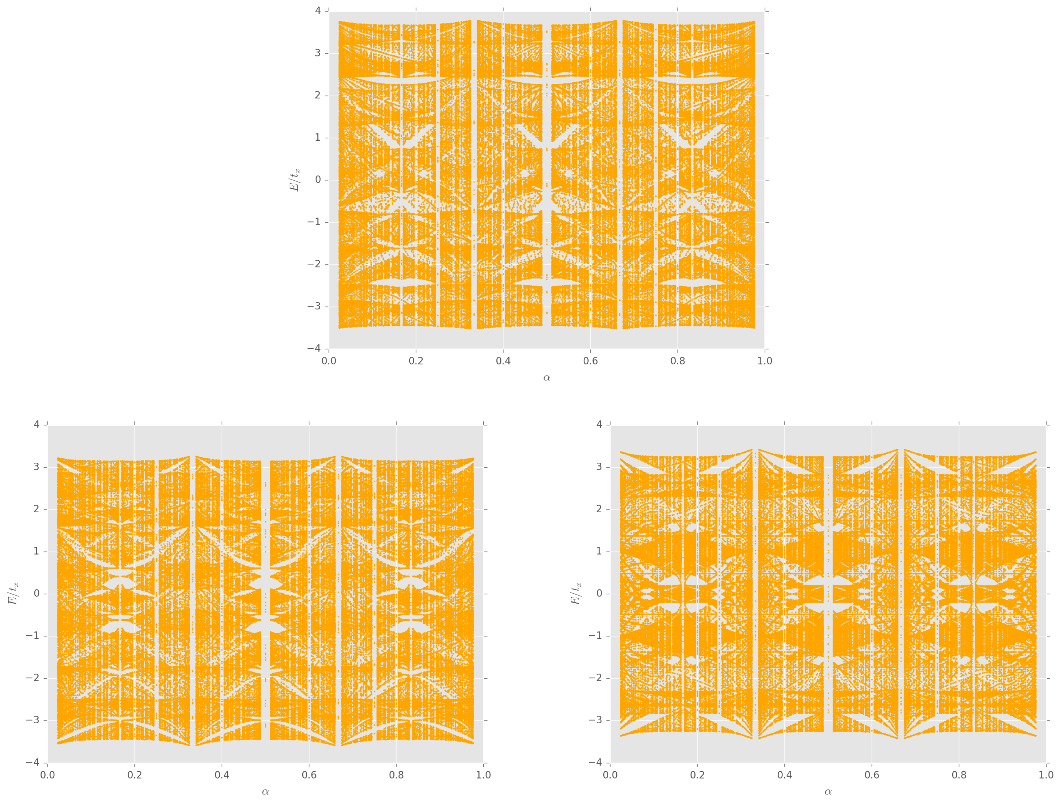
such that the full set of eigenvalues is the union of the eigenvalues obtained for the three decoupled systems. Figure 1 shows the plots of these energy eigenvalues as functions of for and . The three plots, from left to right, correspond to respectively. We have checked that the features of the plots remain unchanged irrespective of whether the horizontal axis is chosen as , or , whilst keeping the other two s fixed.
3.2. Metal–Insulator Transition for Irrational Flux
The Hofstadter system [25] undergoes metal–insulator transitions for irrational values of flux and the spectra do not depend on . For instance, let us assume that . We will approximate this irrational number by the rational approximation . Figure 2 shows the plot of the energy eigenvalues from Equations (12)–(14) as a function of for and . The Abelian case corresponding to has also been shown, which shows bands with no variation along . Also in Figure 3, we show how the minimum energy states for localizes with increasing r.
If we consider the case of such that (other choices remaining the same as in Equation (5)), then for , an irrational value of and , the recursive equations reduce to
The equation is uncoupled and has a similar structure to the Harper equation for the Abelian case. This leads us to infer that there is a metal–insulator transition at , such that corresponds to extended states, while characterises localized states. These two phases are shown in Figure 4.
4. Gauge Potential with Constant Wilson Loop
In this section, we study the effect of the gauge potential given by
where is the same as in Equation (5) but now is proportional to the linear combination of the Gell-Mann matrices for . The tunnelling operators in this case correspond to the following unitary matrices:
Here, Equation (4) gives us , which is position-independent and hence we expect a modified butterfly structure.
4.1. Spectrum for Rational Flux
For , writing the wave-functions in terms of Bloch functions using the same notation as in Equation (10), we arrive at the recursive equations given by
where
This case involves solving a eigenvalue problem given by
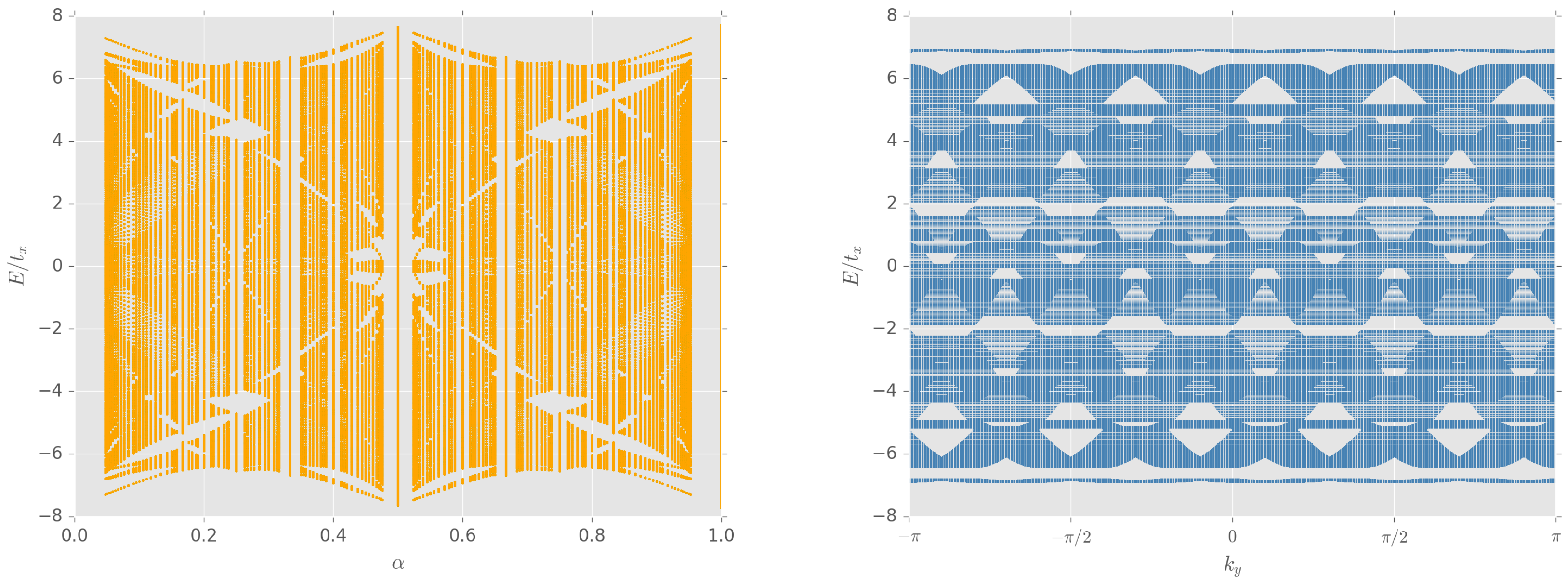
In Figure 5, the energy eigenvalues (with ) have been plotted as a function of (i) α in the left panel, and (ii) for in the right panel.
4.2. Superfluid–Insulator Transition of Ultracold Bosons
We consider three independent species of bosonic ultracold atoms, denoted by , in a square optical lattice. This system is well-captured by the Bose–Hubbard model and has been theoretically shown to undergo superfluid–insulator transitions. Here we study the effect of the gauge potentials given in Equation (16) on such transitions, which result in inter-species hopping terms. Starting from the tight-binding limit, we treat these hopping terms perturbatively. The Hamiltonian of the model is given by
where the interaction strength and the chemical potential μ have been chosen to be the same for all species for simplicity. Here the hopping matrices and are given by Equation (16). We will consider the limit such that describes three independent species having a unique non-degenerate ground state with .
Following the analysis in earlier papers [39,40,41,42], the zeroth order Green’s function (corresponding to ) at zero temperature is given by
where ω is the bosonic Matsubara frequency and () is the energy cost of adding a hole (particle) to the Mott insulating phase. Also, is the on-site particle number.
The x-components of the momenta, in the presence of the flux α, are constrained to lie in the magnetic Brillouin zone where two successive points differ by . For example, can be assigned the discrete values , where . Using this notation, we denote the momentum space wavefunction as . The hopping matrix, obtained from , is then given by
The dispersion relations can be found by solving
where we have analytically continued to real frequencies as . In other words, we have to solve the matrix equation
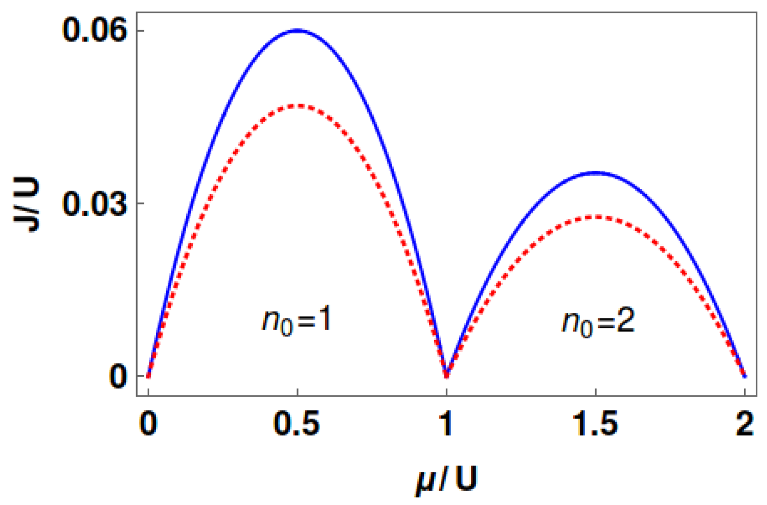
The value of the critical hopping parameter is obtained when the gap between the lowest particle excitation energy and the highest hole excitation energy goes to zero. The Mott lobes for are shown in Figure 6.
5. Discussion
To summarise, we have extended existing studies of ultracold atoms in artificial gauge potentials to the case of . In doing so, we have considered background gauge fields with both non-constant and constant Wilson loops. We find that the spectrum for the constant Wilson loop case exhibits a fractal structure very similar to the well-studied Abelian case of Hofstader’s. Systems with irrational fluxes have been shown to undergo metal–insulator transitions as the hopping parameters are tuned. We have also shown the effect of such a gauge potential in the specific case of the Mott insulator and for superfluid transition for bosonic ultracold atoms subjected to rational flux-values.
There are certain similarities observed with the cases. For the metal-insulator transition in Section 3.2, the behaviour of the extended/localized states in the -r plane are similar to that in the case [32]. Again, for the superfluid-insulator transition in Section 4.2, the presence of the flux led to a suppression of the values of with respect to the zero fluz case. Such suppression was also found in the case [42].
In general, it might be easier to simulate U(2) gauge potentials rather than U(3) or higher gauge group potentials in cold atom experiments. While systems with U(2) gauge potential can be useful to study fermions with the spin degree of freedom, which is what we find in condensed matter systems, the simulation of U(3) gauge potentials may open the path to study QCD-like systems.
Our study opens several pathways towards future work involving these systems. For instance, in the fractal case, the Chern numbers for the emerging energy bands can be calculated leading to the identification of the various topological phases. Further, while for the scope of this work, we have limited ourselves to the simplest case of square lattice, it will be interesting to study cases with other structures such as triangular and honeycomb lattices. Future exploration along these directions will give a better theoretical understanding of such systems. It will also help in optimising design related decisions for experiments in the field and suggest the experimental signatures one ought to go hunting for.
Acknowledgments
I.M. is supported by NSERC of Canada and the Templeton Foundation. A.B. is supported by the Fonds de la Recherche Scientifique-FNRS under grant number 4.4501.15. In addition A.B. is grateful for the hospitality provided by the Perimeter Institute during the completion of the work. Research at the Perimeter Institute is supported, in part, by the Government of Canada through Industry Canada and by the Province of Ontario through the Ministry of Research and Information.
Author Contributions
I.M. conceived and set up the problem and the equations; A.B. wrote numerical codes for solving the equations and plotting the data obtained.
References
- Bloch, I.; Dalibard, J.; Zwerger, W. Many-body physics with ultracold gases. Rev. Mod. Phys. 2008, 80, 885–964. [Google Scholar] [CrossRef]
- Lewenstein, M.; Sanpera, A.; Ahufinger, V.; Damski, B.; Sen, A.; Sen, U. Ultracold atomic gases in optical lattices: mimicking condensed matter physics and beyond. Adv. Phys. 2007, 56, 243–379. [Google Scholar] [CrossRef]
- Juzeliūnas, G.; Ruseckas, J.; Dalibard, J. Generalized Rashba-Dresselhaus spin-orbit coupling for cold atoms. Phys. Rev. A 2010, 81, 053403. [Google Scholar] [CrossRef]
- Dalibard, J.; Gerbier, F.; Juzeliūnas, G.; Öhberg, P. Colloquium: Artificial gauge potentials for neutral atoms. Rev. Mod. Phys. 2011, 83, 1523–1543. [Google Scholar] [CrossRef]
- Banerjee, D.; Dalmonte, M.; Müller, M.; Rico, E.; Stebler, P.; Wiese, U.J.; Zoller, P. Atomic Quantum Simulation of Dynamical Gauge Fields Coupled to Fermionic Matter: From String Breaking to Evolution after a Quench. Phys. Rev. Lett. 2012, 109, 175302. [Google Scholar] [CrossRef] [PubMed]
- Goldman, N.; Satija, I.; Nikolic, P.; Bermudez, A.; Martin-Delgado, M.A.; Lewenstein, M.; Spielman, I.B. Realistic Time-Reversal Invariant Topological Insulators with Neutral Atoms. Phys. Rev. Lett. 2010, 105, 255302. [Google Scholar] [CrossRef] [PubMed]
- Bermudez, A.; Mazza, L.; Rizzi, M.; Goldman, N.; Lewenstein, M.; Martin-Delgado, M.A. Wilson Fermions and Axion Electrodynamics in Optical Lattices. Phys. Rev. Lett. 2010, 105, 190404. [Google Scholar] [CrossRef] [PubMed]
- Mazza, L.; Bermudez, A.; Goldman, N.; Rizzi, M.; Martin-Delgado, M.A.; Lewenstein, M. An optical-lattice-based quantum simulator for relativistic field theories and topological insulators. New J. Phys. 2012, 14, 015007. [Google Scholar] [CrossRef]
- Goldman, N.; Kubasiak, A.; Bermudez, A.; Gaspard, P.; Lewenstein, M.; Martin-Delgado, M.A. Non-Abelian Optical Lattices: Anomalous Quantum Hall Effect and Dirac Fermions. Phys. Rev. Lett. 2009, 103, 035301. [Google Scholar] [CrossRef] [PubMed]
- Bermudez, A.; Goldman, N.; Kubasiak, A.; Lewenstein, M.; Martin-Delgado, M.A. Topological phase transitions in the non-Abelian honeycomb lattice. New J. Phys. 2010, 12, 033041. [Google Scholar] [CrossRef]
- Ho, T.L. Bose–Einstein Condensates with Large Number of Vortices. Phys. Rev. Lett. 2001, 87, 060403. [Google Scholar] [CrossRef] [PubMed]
- Jaksch, D.; Zoller, P. Creation of effective magnetic fields in optical lattices: the Hofstadter butterfly for cold neutral atoms. New J. Phys. 2003, 5, 56. [Google Scholar] [CrossRef]
- Mueller, E.J. Artificial electromagnetism for neutral atoms: Escher staircase and Laughlin liquids. Phys. Rev. A 2004, 70, 041603. [Google Scholar] [CrossRef]
- Sørensen, A.S.; Demler, E.; Lukin, M.D. Fractional Quantum Hall States of Atoms in Optical Lattices. Phys. Rev. Lett. 2005, 94, 086803. [Google Scholar] [CrossRef] [PubMed]
- Juzeliūnas, G.; Öhberg, P.; Ruseckas, J.; Klein, A. Effective magnetic fields in degenerate atomic gases induced by light beams with orbital angular momenta. Phys. Rev. A 2005, 71, 053614. [Google Scholar] [CrossRef] [Green Version]
- Juzeliūnas, G.; Öhberg, P. Slow Light in Degenerate Fermi Gases. Phys. Rev. Lett. 2004, 93, 033602. [Google Scholar] [CrossRef] [PubMed]
- Lin, Y.J.; Compton, R.L.; Jiménez-García, K.; Porto, J.V.; Spielman, I.B. Synthetic magnetic fields for ultracold neutral atoms. Nature 2009, 462, 628–632. [Google Scholar] [CrossRef] [PubMed]
- Lin, Y.J.; Compton, R.L.; Perry, A.R.; Phillips, W.D.; Porto, J.V.; Spielman, I.B. Bose–Einstein Condensate in a Uniform Light-Induced Vector Potential. Phys. Rev. Lett. 2009, 102, 130401. [Google Scholar] [CrossRef] [PubMed]
- Bhat, R.; Holland, M.J.; Carr, L.D. Bose–Einstein Condensates in Rotating Lattices. Phys. Rev. Lett. 2006, 96, 060405. [Google Scholar] [CrossRef] [PubMed]
- Polini, M.; Fazio, R.; MacDonald, A.H.; Tosi, M.P. Realization of Fully Frustrated Josephson-Junction Arrays with Cold Atoms. Phys. Rev. Lett. 2005, 95, 010401. [Google Scholar] [CrossRef] [PubMed]
- Bhat, R.; Krämer, M.; Cooper, J.; Holland, M.J. Hall effects in Bose–Einstein condensates in a rotating optical lattice. Phys. Rev. A 2007, 76, 043601. [Google Scholar] [CrossRef]
- Tung, S.; Schweikhard, V.; Cornell, E.A. Observation of Vortex Pinning in Bose–Einstein Condensates. Phys. Rev. Lett. 2006, 97, 240402. [Google Scholar] [CrossRef] [PubMed]
- Klein, A.; Jaksch, D. Phonon-induced artificial magnetic fields in optical lattices. Europhys. Lett. 2009, 85, 13001. [Google Scholar] [CrossRef]
- Hu, Y.X.; Miniatura, C.; Wilkowski, D.; Grémaud, B. U(3) artificial gauge fields for cold atoms. Phys. Rev. A 2014, 90, 023601. [Google Scholar] [CrossRef]
- Hofstadter, D.R. Energy levels and wave functions of Bloch electrons in rational and irrational magnetic fields. Phys. Rev. B 1976, 14, 2239–2249. [Google Scholar] [CrossRef]
- Goldman, N. Spatial patterns in optical lattices submitted to gauge potentials. Europhys. Lett. 2007, 80, 20001. [Google Scholar] [CrossRef]
- Palmer, R.N.; Jaksch, D. High-Field Fractional Quantum Hall Effect in Optical Lattices. Phys. Rev. Lett. 2006, 96, 180407. [Google Scholar] [CrossRef] [PubMed]
- Goldman, N.; Gaspard, P. Quantum Hall-like effect for cold atoms in non-Abelian gauge potentials. Europhys. Lett. 2007, 78, 60001. [Google Scholar] [CrossRef]
- Hafezi, M.; Sørensen, A.S.; Lukin, M.D.; Demler, E. Characterization of topological states on a lattice with Chern number. Europhys. Lett. 2008, 81, 10005. [Google Scholar] [CrossRef]
- Osterloh, K.; Baig, M.; Santos, L.; Zoller, P.; Lewenstein, M. Cold Atoms in Non-Abelian Gauge Potentials: From the Hofstadter “Moth” to Lattice Gauge Theory. Phys. Rev. Lett. 2005, 95, 010403. [Google Scholar] [CrossRef] [PubMed]
- Ruseckas, J.; Juzeliūnas, G.; Öhberg, P.; Fleischhauer, M. Non-Abelian Gauge Potentials for Ultracold Atoms with Degenerate Dark States. Phys. Rev. Lett. 2005, 95, 010404. [Google Scholar] [CrossRef] [PubMed]
- Satija, I.I.; Dakin, D.C.; Vaishnav, J.Y.; Clark, C.W. Physics of a two-dimensional electron gas with cold atoms in non-Abelian gauge potentials. Phys. Rev. A 2008, 77, 043410. [Google Scholar] [CrossRef]
- Jacob, A.; Öhberg, P.; Juzeliūnas, G.; Santos, L. Landau levels of cold atoms in non-Abelian gauge fields. New J. Phys. 2008, 10, 045022. [Google Scholar] [CrossRef]
- Jacob, A.; Öhberg, P.; Juzeliūnas, G.; Santos, L. Cold atom dynamics in non-Abelian gauge fields. Appl. Phys. B Lasers Opt. 2007, 89, 439–445. [Google Scholar] [CrossRef]
- Juzeliūnas, G.; Ruseckas, J.; Jacob, A.; Santos, L.; Öhberg, P. Double and Negative Reflection of Cold Atoms in Non-Abelian Gauge Potentials. Phys. Rev. Lett. 2008, 100, 200405. [Google Scholar] [CrossRef] [PubMed]
- Barnett, R.; Boyd, G.R.; Galitski, V. SU(3) Spin-Orbit Coupling in Systems of Ultracold Atoms. Phys. Rev. Lett. 2012, 109, 235308. [Google Scholar] [CrossRef] [PubMed]
- Graß, T.; Chhajlany, R.W.; Muschik, C.A.; Lewenstein, M. Spiral spin textures of a bosonic Mott insulator with SU(3) spin-orbit coupling. Phys. Rev. B 2014, 90, 195127. [Google Scholar] [CrossRef]
- Goldman, N.; Kubasiak, A.; Gaspard, P.; Lewenstein, M. Ultracold atomic gases in non-Abelian gauge potentials: The case of constant Wilson loop. Phys. Rev. A 2009, 79, 023624. [Google Scholar] [CrossRef]
- Sengupta, K.; Dupuis, N. Mott-insulator–to–superfluid transition in the Bose–Hubbard model: A strong-coupling approach. Phys. Rev. A 2005, 71, 033629. [Google Scholar] [CrossRef]
- Freericks, J.K.; Krishnamurthy, H.R.; Kato, Y.; Kawashima, N.; Trivedi, N. Strong-coupling expansion for the momentum distribution of the Bose–Hubbard model with benchmarking against exact numerical results. Phys. Rev. A 2009, 79, 053631. [Google Scholar] [CrossRef]
- Sinha, S.; Sengupta, K. Superfluid-insulator transition of ultracold bosons in an optical lattice in the presence of a synthetic magnetic field. Europhys. Lett. 2011, 93, 30005. [Google Scholar] [CrossRef]
- Graß, T.; Saha, K.; Sengupta, K.; Lewenstein, M. Quantum phase transition of ultracold bosons in the presence of a non-Abelian synthetic gauge field. Phys. Rev. A 2011, 84, 053632. [Google Scholar] [CrossRef]
Figure 1.
The energy eigenvalues of the system depicted by Equation (11) for and as a function of . The three plots correspond to (top), (bottom left) and (bottom right).
Figure 1.
The energy eigenvalues of the system depicted by Equation (11) for and as a function of . The three plots correspond to (top), (bottom left) and (bottom right).

Figure 2.
Energy spectrum from Equations (12)–(14), as a function of for and . and have been plotted in green, blue and orange respectively. The Abelian case corresponding to has also been plotted in grey, which shows bands with no variation with .
Figure 2.
Energy spectrum from Equations (12)–(14), as a function of for and . and have been plotted in green, blue and orange respectively. The Abelian case corresponding to has also been plotted in grey, which shows bands with no variation with .
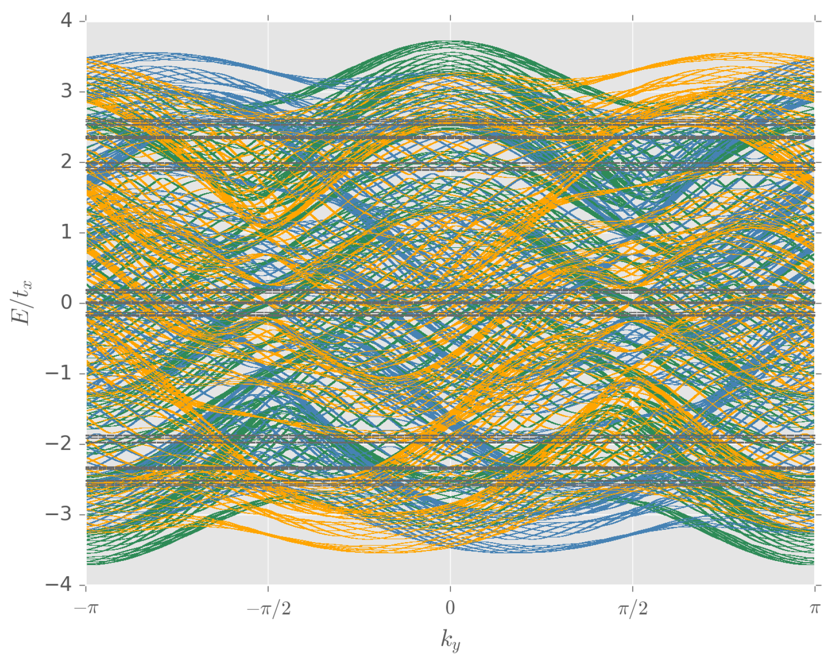
Figure 3.
The behaviour of the system depicted by Equation (10) for irrational flux, captured by plotting the square root of the modulus of the Fourier transform of the wavefunction for the state with minimum energy when as a function of with () for left (right) panel. The four figures in each panel, from top to bottom, show how the state localizes with increasing r.
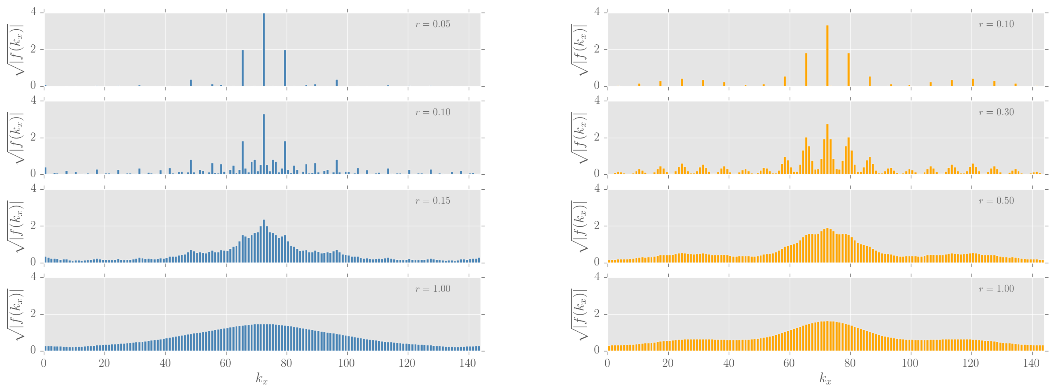
Figure 4.
The metallic (red) and insulating phases (blue) for the system from Equation (14) in the plane.
Figure 4.
The metallic (red) and insulating phases (blue) for the system from Equation (14) in the plane.
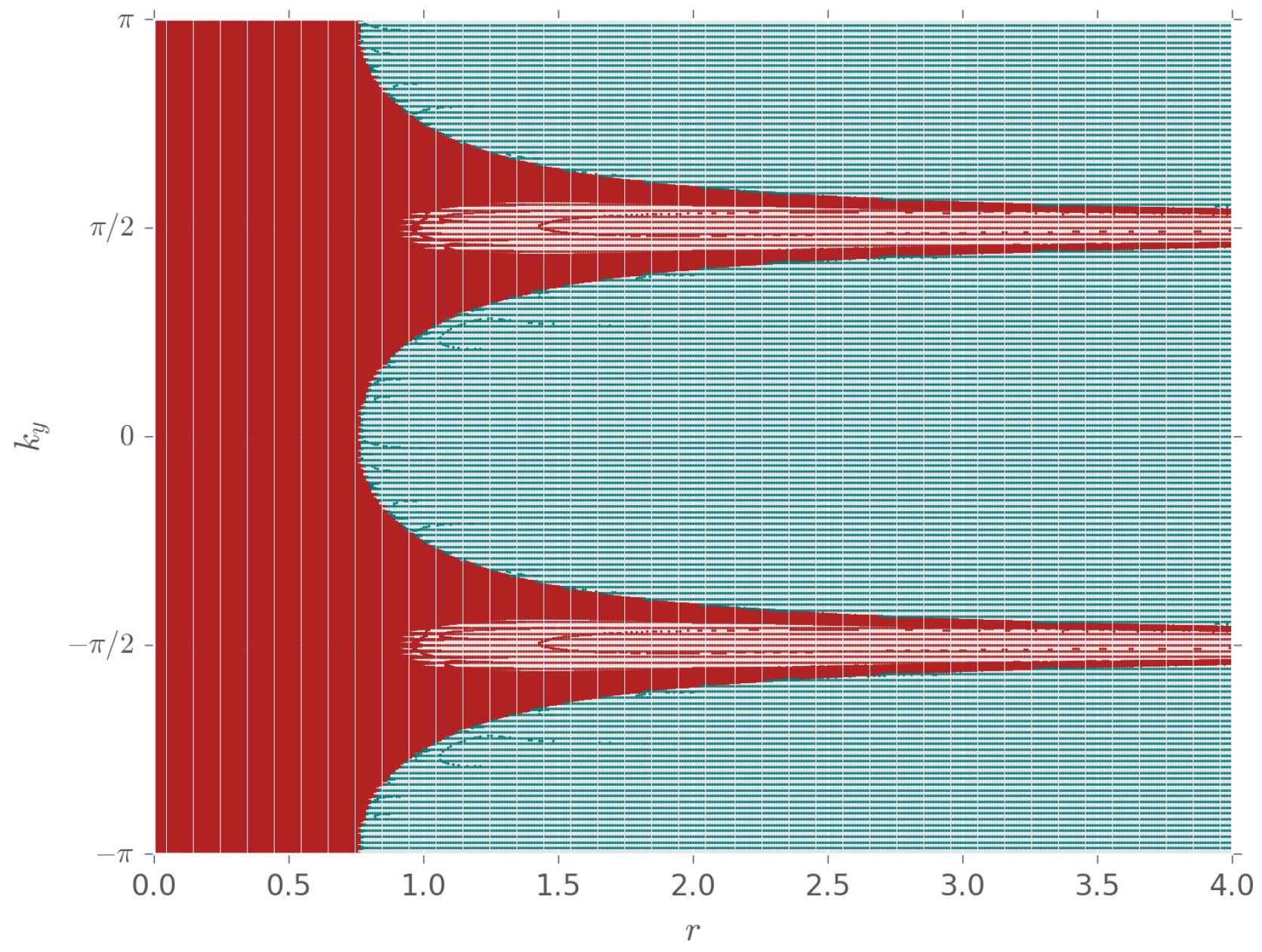
Figure 5.
Energy spectrum from Equation (19) for as a function of (i) α in the left panel, and (ii) at in the right panel.
Figure 5.
Energy spectrum from Equation (19) for as a function of (i) α in the left panel, and (ii) at in the right panel.

Figure 6.
The Mott lobes obtained from the critical values of . The solid blue (dotted red) curve corresponds to .
Figure 6.
The Mott lobes obtained from the critical values of . The solid blue (dotted red) curve corresponds to .

© 2016 by the authors; licensee MDPI, Basel, Switzerland. This article is an open access article distributed under the terms and conditions of the Creative Commons Attribution (CC-BY) license ( http://creativecommons.org/licenses/by/4.0/).
Share and Cite
MDPI and ACS Style
Mandal, I.; Bhattacharya, A. Cold Atoms in U(3) Gauge Potentials. Condens. Matter 2016, 1, 2. https://doi.org/10.3390/condmat1010002
AMA Style
Mandal I, Bhattacharya A. Cold Atoms in U(3) Gauge Potentials. Condensed Matter. 2016; 1(1):2. https://doi.org/10.3390/condmat1010002
Chicago/Turabian StyleMandal, Ipsita, and Atri Bhattacharya. 2016. "Cold Atoms in U(3) Gauge Potentials" Condensed Matter 1, no. 1: 2. https://doi.org/10.3390/condmat1010002