
Goldstone and Higgs Hydrodynamics in the BCS–BEC Crossover


1
Dipartimento di Fisica e Astronomia “Galileo Galilei” and CNISM, Università di Padova, Via Marzolo 8, 35131 Padova, Italy
2
Istituto Nazionale di Ottica (INO) del Consiglio Nazionale delle Ricerche (CNR), Via Nello Carrara 1, 50019 Sesto Fiorentino, Italy
Condens. Matter 2017, 2(2), 22; https://doi.org/10.3390/condmat2020022
Submission received: 23 April 2017
/
Revised: 7 June 2017
/
Accepted: 7 June 2017
/
Published: 20 June 2017
(This article belongs to the Special Issue Control and Enhancement of Quantum Coherence in Nanostructured Materials)
Abstract
:We discuss the derivation of a low-energy effective field theory of phase (Goldstone) and amplitude (Higgs) modes of the pairing field from a microscopic theory of attractive fermions. The coupled equations for Goldstone and Higgs fields are critically analyzed in the Bardeen–Cooper–Schrieffer (BCS)-to-Bose–Einstein condensate (BEC) crossover—both in three spatial dimensions and in two spatial dimensions. The crucial role of pair fluctuations is investigated, and the beyond-mean-field Gaussian theory of the BCS–BEC crossover is compared with available experimental data of the two-dimensional ultracold Fermi superfluid.
1. Introduction
An important achievement in the physics of ultracold atoms was the experimental realization of the crossover from the Bardeen–Cooper–Schrieffer (BCS) superfluid phase of loosely-bound pairs of fermions to the Bose–Einstein condensate (BEC) of tightly-bound composite bosons [1,2]. Superfluid fermions in the BCS–BEC crossover are an ideal platform to investigate macroscopic quantum phenomena. For instance, macroscopic quantum tunneling and quantum self-trapping [3,4,5] have recently been observed across the BCS–BEC crossover [6].
Very recently, the BCS–BEC crossover has also been realized in quasi two-dimensional (2D) configurations [7,8,9,10]. Beyond-mean-field theoretical investigations of 2D Fermi gases in the full BCS–BEC crossover have been carried out both at zero and finite temperature [11,12,13,14,15,16,17]. These 2D results have clearly shown that contrary to the 3D case, mean-field theories are completely unreliable for the study of strongly-interacting superfluid fermions in two dimensions because of the huge increase of quantum fluctuations. The 2D BCS–BEC crossover is also interesting for high-T superconductivity where the phase diagram of cuprate superconductors can be interpreted in terms of a BCS–BEC crossover as doping is varied. The critical temperature T has a wide fluctuation region with pseudo-gap effects not yet fully understood [18,19]. Moreover, it has been suggested that iron-based superconductors have composite superconductivity, consisting of strong-coupling BEC in the electron band and weak-coupling BCS-like superconductivity in the hole band [20].
This year, we have used renormalization-group techniques to calculate the Berezinskii–Kosterlitz–Thouless (BKT) critical temperature [21,22], taking explicitly into account the formation of quantized vortices [23]. The presence of quantized vortices and antivortices renormalizes the superfluid density of the system as the temperature increases, and the renormalized superfluid density jumps from a finite value to zero as the temperature reaches the BKT critical temperature [24]. In this way, we have also obtained the BKT critical temperature in the full 2D BCS–BEC crossover for the uniform Fermi superfluid [23]. Quantized vortices in superfluids are a peculiar consequence of the existence of an underlying compact real field, whose spatial gradient determines the local superfuid velocity of the system [25,26,27]. This compact real field—the so-called Goldstone field—is the phase angle of the complex bosonic field which in the case of attractive fermions describes strongly-correlated Cooper pairs of fermions with opposite spins. The amplitude of this complex pairing field—sometimes also called a Higgs field [28]—is decoupled from the angular Goldstone field only in the deep BCS regime where the particle–hole symmetry is almost preserved.
In this paper, we review the low-energy effective field theory of Goldstone and Higgs modes derived from the microscopic theory of paired fermions. At zero temperature, we show that the velocity of the Goldstone mode obtained with and without amplitude fluctuations (in 2D but also in 3D) has a quite different behavior [11]. We find that amplitude fluctuations are necessary to identify the velocity of the Goldstone mode with the first sound velocity one gets from the mean-field equation of state by using familiar thermodynamics relationships [11]. Finally, we show that in the 2D case, the first sound velocity obtained from the beyond-mean-field equation of state is quite different with respect to the mean-field one—in particular in the BEC side of the BCS–BEC crossover [15]. For the sake of completeness, we also report our beyond-mean-field calculation [13,14,15,16] of the zero-temperature pressure of the Fermi superfluid in the 2D BCS–BEC crossover: these theoretical results are in very good agreement with the available experimental data [7].
2. Functional Integration for the BCS–BEC Crossover
We consider a D-dimensional system of two-spin-component fermions interacting through an attractive s-wave contact potential, contained in a volume V, at fixed chemical potential and temperature T. Within the path integral formalism, the partition function of the system can be written as [25,26,27]
where , are complex Grassmann fields (), , with is Boltzmann constant, and the Euclidean Lagrangian density reads
Here g is the attractive interaction strength () of the s-wave coupling between fermions with opposite spin . Looking for analytical solutions, the quartic interaction cannot be treated exactly. The Hubbard–Stratonovich transformation [25,26,27] introduces an additional auxiliary pairing field corresponding to a Cooper pair, decoupling the quartic interaction. The transformation is based on the following identity
The partition function can then be written as
with the following Lagrangian density
The integration over the fermionic fields and can now be carried out exactly, obtaining
with the inverse Green’s function, given by
To investigate effects of quantum and thermal fluctuations of the gap field around its mean-field value , we set
where is the complex field of pairing fluctuations. In this way, the inverse Green function is decomposed in a mean-field component , where the pairing field is replaced by its uniform and constant saddle point value, plus a fluctuation part :
2.1. Loop Expansion and Gaussian Approximation
The Gaussian (one-loop) approximation consists of the following expansion for the second term in the right-hand-side of Equation (10):
Within this Gaussian approximation, the partition function reads
where
is the mean-field partition function and
is the Gaussian partition function characterized by the following Gaussian action:
In this formula, we have introduced the Fourier transform of the fluctuation fields and the bosonic Matsubara frequencies . The matrix elements of the inverse pair fluctuation propagator are given by [29]
and
where
is the spectrum of fermionic single-particle excitations.
2.2. Beyond-Mean-Field Grand Potential
The thermodynamic grand potential of the fermionic superfluid is given by
The Gaussian grand potential is instead
The sum over Matsubara frequencies is quite complicated, and it does not give a simple expression. An approximate formula which is valid in the BEC regime of the crossover [30] is the following:
where
is the spectrum of bosonic collective excitations with derived from
In the Gaussian pair fluctuation (GPF) approach [31], given the grand potential
the energy gap is obtained from the mean-field gap equation
The number density n is instead obtained from the beyond-mean-field number equation
taking into account the gap equation (i.e., that depends on and T: ). Notice that the Nozieres and Schmitt–Rink approaches [32] are quite similar, but in the number equation one forgets that depends on .
3. Low-Energy Gaussian Action
We have seen that the analytical form of the inverse pair fluctuation propagator (with ) is quite complicated, and one can find its matrix elements numerically. Here we use a series expansion of up to the second order in and [33,34,35]. Moreover, we decompose the fluctuation field as follows:
where and are real and can be identified at the lowest order with amplitude and phase fluctuations, respectively [33,34,35]. In other words, is the Higgs field and is the Goldstone field [28].
In this way, after some calculations [11,34,35], one finds the low-energy real-time Gaussian action derived from the Euclidean Gaussian action (15)
where is the real time. At zero temperature, the coefficients J, , , and are related to the partial derivatives of the zero-temperature mean-field grand potential [11,35]. In particular,
is the phase stiffness,
is the phase–phase susceptibility,
is the amplitude–amplitude susceptibility, and
is the phase–amplitude susceptibility, that is the Goldstone–Higgs coupling constant. Equation (30) is practically the same action functional derived in [36,37] by using a two-channel model model for the BCS–BEC crossover.
Calculating the time derivative of from Equation (36), one finds
Inserting this result in Equation (35), we finally get the d’Alambert equation of waves
which admits the generic solution
with the dispersion relation
and
the velocity of propagation of the Goldstone mode, where
is the effective susceptibility. Notice that only if the amplitude fluctuations are negligible (i.e., ); from Equation (36), it follows and consequently .
In the 3D BCS–BEC crossover, the interaction strength g is usually written in terms of the to 3D s-wave scattering length a [27]
Instead, in the 2D BCS–BEC crossover, the interaction strength g is usually related to the binding energy of Cooper pairs by [16]
In fact, contrary to the 3D case, 2D realistic interatomic attractive potentials always have a bound state. Both Equations (43) and (44) are ultraviolet divergent, but they exactly compensate the divergence of the mean-field grand potential , which depends of the bare interaction strength g [16].
Figure 1 shows that taking into account only phase fluctuations (i.e., setting ) leads to a quite different behaviour of the velocity from that obtained by considering both phase and amplitude fluctuations [11]. In the Figure 1a, there is the behaviour of in the 2D BCS–BEC crossover, while in the Figure 1b there are the results for the 3D BCS–BEC crossover. Only in the deep BCS regime (left side of the two panels of Figure 1) do the two approaches give the same results, while the phase-only sound velocity diverges in the BEC regime (right side of panels). Thus, the effect of Goldstone–Higgs coupling is crucial in the study of the BCS–BEC crossover. It is important to stress that the zero-temperature results of Figure 1 are obtained adopting the mean-field number equation; i.e.,
We used Equation (45) instead of Equation (28) in the calculation of in order to have, from Equation (31),
which is the expected phase stiffness at zero temperature, where the total density n should be equal to the superfluid density . In this way, one also satisfies the compressibility sum rule [38].
3.1. Connection with the Popov’s Hydrodynamic Action Functional
Given the Goldstone–Higgs action functional (30) and performing functional integration over the Higgs field , one obtains the Goldstone action
whose Euler–Lagrange equation is exactly Equation (38) with K given by Equation (42). Remarkably, this Goldstone action functional can be immediately derived from the Popov’s hydrodynamic action [39]
functional integrating over the field of density fluctuations. represents a small space-time-dependent perturbation with respect to the constant and uniform density n. In the zero-temperature action functional (48), both J and K depend on n through the relationship between and n. From the Euler–Lagrange equations of (48) with respect to and , and introducing the velocity field
one finds the familiar linearized hydrodynamic equations of Euler
from which one immediately finds the d’Alambert equation for density fluctuations
Thus, one can identify the velocity of propagation of the Goldstone mode with the velocity of the first sound of the fermionic superfluid [25,26,27]. In fact, according to the two-fluid theory of Laudau [40], a superfluid is characterized by the presence of the first sound (where superfluid and normal components oscillate in phase), but also the second sound, where superfluid and normal components oscillate with opposite phases. For the sake of completeness, we observe that the Euler Equations (50) and (51) can also be re-written in terms of a nonlinear Schrödinger equation for the complex field [36,37,41,42].
3.2. First Sound Velocity from Thermodynamics
On the basis of the two-fluid theory [40,43], at zero temperature the first sound velocity of a superfluid is simply given by
where is the chemical potential, n is the number density, and V is the volume. Refs. [11,44] have shown that the velocity of the Goldstone mode given by Equation (41) coincides with the first sound velocity , given by Equation (53), if one uses the mean-field equation of state (45).
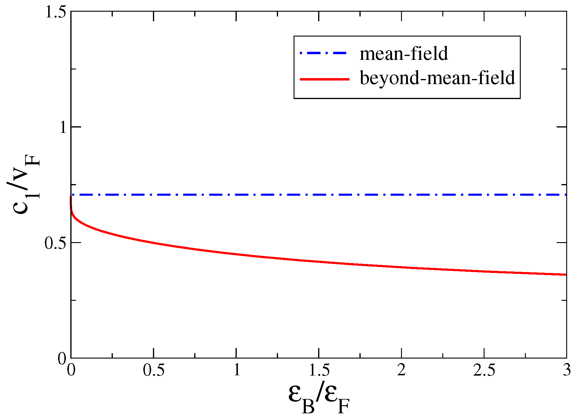
At zero temperature, the difference between Equations (28) and (45) is small in the 3D case, but it is instead very large in the 2D case, and in particular in the BEC regime of the crossover [15]. This effect is clearly shown in Figure 2, where we report the zero-temperature first sound velocity in the 2D BCS–BEC crossover, regulated by the binding energy of Cooper pairs. In Figure 2, the dot-dashed line is obtained by using the mean-field number Equation (45), while the solid line is based on the beyond-mean-field number Equation (28). In the strong coupling BEC regime, the beyond-mean-field equation of state is needed to accurately describe the thermodynamic quantities, and the corresponding first found velocity correctly goes to the correct composite boson limit [12].
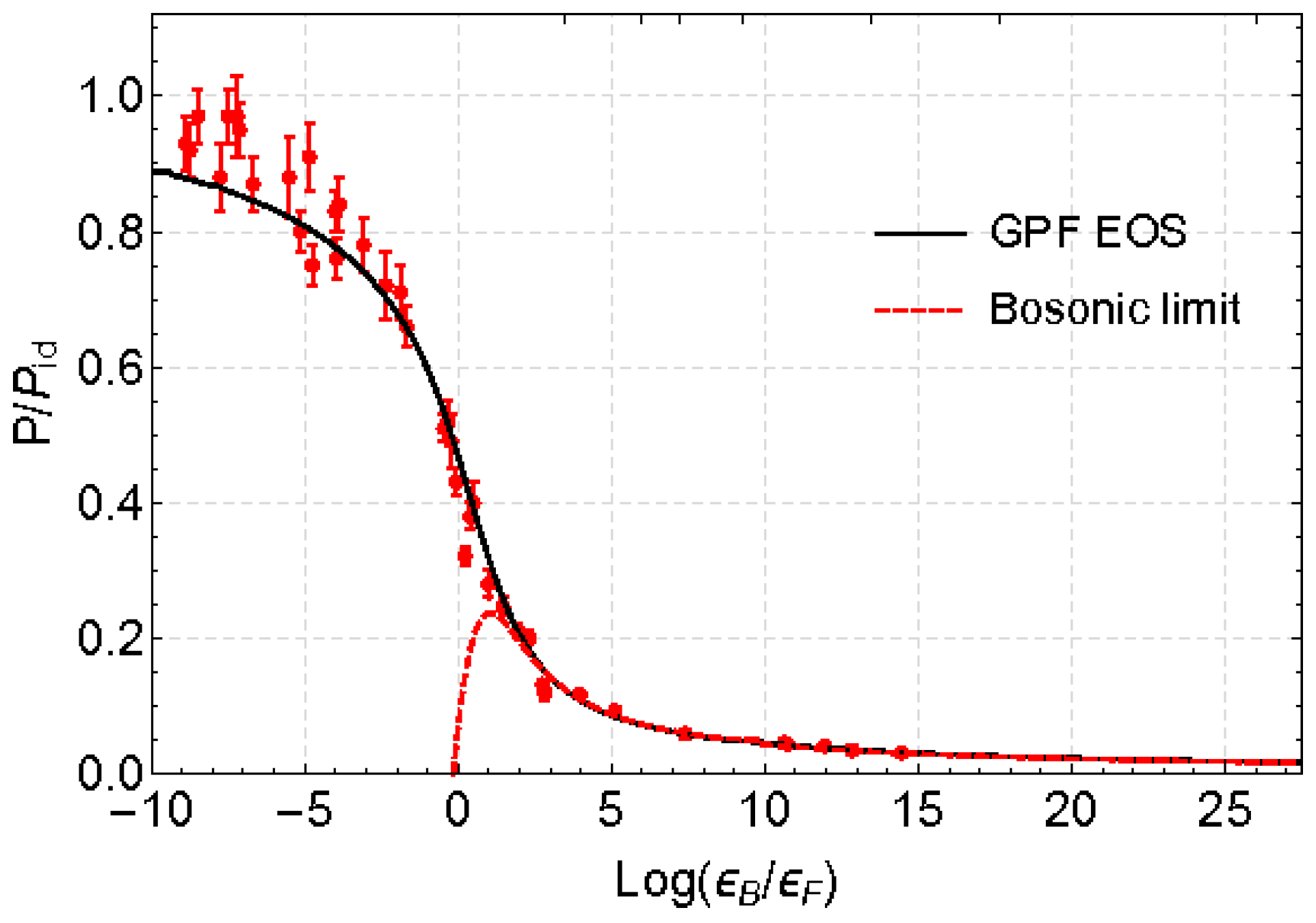
Bighin and Salasnich [15] have shown that the first sound velocity obtained with the beyond-mean-field Gaussian theory (solid line of Figure 2) is in good agreement with very preliminary experimental data of Li atoms [45]. Unfortunately, there are not yet fully reliable published experimental data on the sound velocity . However, there are reliable experimental data of the pressure P at very low temperature for the dilute gas of Li atoms [7]. In Figure 3, we plot these experimental data (filled circles with error bars) and compare them with our beyond-mean-field theory at zero temperature (solid line). The pressure is immediately obtained as
with given by Equation (26). Figure 3 clearly shows that, at zero temperature, the agreement between experimental data and our beyond-mean-field theory is very good in the full BCS–BEC crossover. In the deep BEC regime, the beyond-mean-field pressure becomes [12]
This formula (dashed line of Figure 3) is nothing else than the Popov equation of state [46] of weakly-interacting repulsive bosons
where is the mass of composite bosons and is the bosonic chemical potential. Note that very recently we have obtained non-universal corrections to the Popov equation of state, taking account of finite-range effects of the inter-atomic potential [47].
4. Conclusions
We have analyzed the derivation of a low-energy effective field theory of Goldstone and Higgs fields from the beyond-mean-field BCS theory of attractive fermions. We have shown that across the BCS–BEC crossover, the inclusion of the Goldstone–Higgs coupling is crucial to identify the velocity of the Goldstone mode with the first sound velocity one gets from the mean-field equation of state. Moreover, we have explicitly shown that in the BEC side of the 2D BCS–BEC crossover, the first sound velocity obtained from the beyond-mean-field equation of state is quite different with respect to the mean-field one. Finally, comparing our theoretical results with 2D experimental data, we have found that at zero temperature the beyond-mean-field theory based on Gaussian pair fluctuations seems reliable in the full 2D BCS–BEC crossover, giving the Popov equation of state in the deep BEC regime. However, as shown in [48,49], at low temperatures and in the deep BCS regime, quantized vortices and dark solitons obtained with effective field approaches based on low-energy expansion may contradict with the Bogoliubov-de Gennes theory, which is well-founded in the BCS regime.
Conflicts of Interest
The author declares no conflict of interest.
References
- Greiner, M.; Regal, C.A.; Jin, D.S. Emergence of a Molecular Bose-Einstein Condensate from a Fermi Gas. Nature 2003, 426, 537–540. [Google Scholar] [CrossRef] [PubMed]
- Chin, C.; Bartenstein, M.; Altmeyer, A.; Riedl, S.; Jochim, S.; Hecker Denschlag, J.; Grimm, R. Observation of the Pairing Gap in a Strongly Interacting Fermi Gas. Science 2004, 305, 1128–1130. [Google Scholar] [CrossRef] [PubMed]
- Smerzi, A.; Fantoni, S.; Giovanazzi, S.; Shenoy, S.R. Quantum coherent atomic tunneling between two trapped Bose-Einstein condensates. Phys. Rev. Lett. 1997, 79, 4950. [Google Scholar] [CrossRef]
- Salasnich, L.; Parola, A.; Reatto, L. Bose condensate in a double-well trap: Ground state and elementary excitations. Phys. Rev. A 1999, 60, 4171–4174. [Google Scholar] [CrossRef]
- Salasnich, L.; Manini, N.; Toigo, F. Macroscopic periodic tunneling of Fermi atoms in the BCS-BEC crossover. Phys. Rev. A 2008, 77, 043609. [Google Scholar] [CrossRef]
- Valtolina, G.; Burchianti, A.; Amico, A.; Neri, E.; Xhani, K.; Seman, J.A.; Trombettoni, A.; Smerzi, A.; Zaccanti, A.; Inguscio, M.; et al. Josephson effect in fermionic superfluids across the BEC-BCS crossover. Science 2016, 350, 1505–1508. [Google Scholar] [CrossRef] [PubMed]
- Makhalov, V.; Martiyanov, K.; Turlapov, A. Ground-state pressure of quasi-2D Fermi and Bose gases. Phys. Rev. Lett. 2014, 112, 045301. [Google Scholar] [CrossRef] [PubMed]
- Murthy, P.A.; Boettcher, I.; Bayha, L.; Holzmann, M.; Kedar, D.; Neidig, M.; Ries, M.G.; Wenz, A.N.; Zurn, G.; Jochim, S. Observation of the Berezinskii-Kosterlitz-Thouless phase transition in an ultracold Fermi gas. Phys. Rev. Lett. 2015, 115, 010401. [Google Scholar] [CrossRef] [PubMed]
- Fenech, K.; Dyke, P.; Peppler, T.; Lingham, M.G.; Hoinka, S.; Hu, H.; Vale, C.J. Thermodynamics of an attractive 2D Fermi gas. Phys. Rev. Lett. 2016, 116, 045302. [Google Scholar] [CrossRef] [PubMed]
- Boettcher, I.; Bayha, L.; Kedar, D.; Murthy, P.A.; Neidig, M.; Ries, M.G.; Wenz, A.N.; Zurn, G.; Jochim, S.; Enss, T. Equation of state of ultracold fermions in the 2D BEC-BCS crossover. Phys. Rev. Lett. 2016, 116, 045303. [Google Scholar] [CrossRef] [PubMed]
- Salasnich, L.; Marchetti, P.A.; Toigo, F. Superfluidity, sound velocity, and quasicondensation in the two-dimensional BCSBEC crossover. Phys. Rev. A 2013, 88, 053612. [Google Scholar] [CrossRef]
- Salasnich, L.; Toigo, F. Composite bosons in the two-dimensional BCS-BEC crossover from Gaussian fluctuations. Phys. Rev. A 2015, 91, 011604. [Google Scholar] [CrossRef]
- He, L.; Lv, H.; Cao, G.; Hu, H.; Liu, X.-J. Quantum fluctuations in the BCS-BEC crossover of two-dimensional Fermi gases. Phys. Rev. A 2015, 92, 023620. [Google Scholar] [CrossRef]
- Mulkerin, B.C.; Fenech, K.; Dyke, P.; Vale, C.J.; Liu, X.-J.; Hu, H. Comparison of strong-coupling theories for a two-dimensional Fermi gas. Phys. Rev. A 2015, 92, 063636. [Google Scholar] [CrossRef]
- Bighin, G.; Salasnich, L. Finite-temperature quantum fluctuations in two-dimensional Fermi superfluids. Phys. Rev. B 2016, 93, 014519. [Google Scholar] [CrossRef]
- Salasnich, L.; Toigo, F. Zero-point energy of ultracold atoms. Phys. Rep. 2016, 640, 1–29. [Google Scholar] [CrossRef]
- Mulkerin, B.C.; He, L.; Dyke, P.; Vale, C.J.; Hu, H. Superfluid Density and Critical Velocity Near the Fermionic Berezinskii–Kosterlitz–Thouless Transition. Available online: http://arxiv.org/abs/1702.07091 (accessed on 30 May 2017).
- Larkin, A.; Varlamov, A. Theory of Fluctuations in Superconductors; Oxford University Press: Oxford, UK, 2005. [Google Scholar]
- Chen, Q.; Stajic, J.; Tan, S.; Levin, K. BCS–BEC crossover: From high temperature superconductors to ultracold superfluids. Phys. Rep. 2005, 412, 1–88. [Google Scholar] [CrossRef]
- Okazaji, K.; Ito, Y.; Ota, Y.; Kotani, Y.; Shimojima, T.; Kiss, T.; Watanabe, S.; Chen, C.-T.; Niitaka, S.; Hanaguri, T.; et al. Superconductivity in an electron band just above the Fermi level. Sci. Rep. 2014, 4, 4109. [Google Scholar] [CrossRef] [PubMed]
- Berezinskii, V.L. Destruction of long-range order in one-dimensional and two-dimensional systems possessing a continuous symmetry group. II. Quantum systems. Sov. Phys. JETP 1972, 34, 610–616. [Google Scholar]
- Kosterlitz, J.M.; Thouless, D.J. Ordering, metastability and phase transitions in two-dimensional systems. J. Phys. C Solid State Phys. 1973, 6, 1181–1203. [Google Scholar] [CrossRef]
- Bighin, G.; Salasnich, L. Vortices and antivortices in two-dimensional ultracold Fermi gases. Sci. Rep. 2017, 7, 45702. [Google Scholar] [CrossRef] [PubMed]
- Nelson, D.R.; Kosterlitz, J.M. Universal jump in the superfluid density of two-dimensional superfluids. Phys. Rev. Lett. 1977, 39, 1201–1205. [Google Scholar] [CrossRef]
- Nagaosa, N. Quantum Field Theory in Condensed Matter Physics; Springer: Berlin, Germany, 1999. [Google Scholar]
- Altland, A.; Simons, B. Condensed Matter Field Theory; Cambridge University Press: Cambridge, UK, 2006. [Google Scholar]
- Stoof, H.T.C.; Gubbels, K.B.; Dickerscheid, D.B.M. Ultracold Quantum Fields; Springer: Dordrecht, The Netherlands, 2009. [Google Scholar]
- Pekker, D.; Varma, C.M. Amplitude/Higgs modes in condensed matter physics. Annu. Rev. Condens. Matter Phys. 2015, 6, 269–297. [Google Scholar] [CrossRef]
- Tempere, J.; Devreese, J.P.A. Superconductors—Materials, Properties and Applications; InTech: Rijeka, Croatia, 2012; pp. 1–32. [Google Scholar]
- Taylor, E.; Griffin, A.; Fukushima, N.; Ohashi, Y. Pairing fluctuations and the superfluid density through the BCS-BEC crossover. Phys. Rev. A 2006, 74, 063626. [Google Scholar] [CrossRef]
- Hu, H.; Liu, X.-J.; Drummond, P.D. Equation of state of a superfluid Fermi gas in the BCS-BEC. Europhys. Lett. 2006, 74, 574–580. [Google Scholar] [CrossRef]
- Nozieres, P.; Schmitt-Rink, S. Bose condensation in an attractive fermion gas: From weak to strong coupling superconductivity. J. Low Temp. Phys. 1985, 59, 195–211. [Google Scholar] [CrossRef]
- Engelbrecht, J.R.; Randeria, M.; Sa de Melo, C.A.R. BCS to Bose crossover: Broken-symmetry state. Phys. Rev. B 1997, 55, 15153–15156. [Google Scholar] [CrossRef]
- Diener, R.B.; Sensarma, R.; Randeria, M. Quantum Fluctuations in the Superfluid State of the BCS-BEC Crossover. Phys. Rev. A 2008, 77, 023626. [Google Scholar] [CrossRef]
- Schakel, A.M.J. Derivation of the effective action of a dilute Fermi gas in the unitary limit of the BCS-BEC crossover. Ann. Phys. 2011, 326, 193–206. [Google Scholar] [CrossRef]
- Lin, C.-Y.; Lee, D.-S.; Rivers, R.J. Spontaneous vortex production in driven condensates with narrow Feschbach resonances. Phys. Rev. A 2011, 84, 013623. [Google Scholar] [CrossRef]
- Hsiang, J.-T.; Lin, C.-Y.; Lee, D.-S.; Rivers, R.J. The role of causality in tunable Fermi gas condensates. J. Phys. Condens. Matter 2013, 25, 404211. [Google Scholar] [CrossRef] [PubMed]
- Anderson, B.M.; Boyack, R.; Wu, C.-T.; Levin, K. Correcting inconsistencies in the conventional superfluid path integral scheme. Phys. Rev. B 2016, 93, 180504. [Google Scholar] [CrossRef]
- Popov, V.N. Functional Integrals in Quantum Field Theory and Statistical Physics; Reidel: Dordrecht, The Netherlands, 1983. [Google Scholar]
- Landau, L.D. The theory of superfuidity of helium II. Phys. Rev. 1941, 60, 356–358. [Google Scholar] [CrossRef]
- Salasnich, L.; Toigo, F. Extended Thomas-Fermi density functional for the unitary Fermi gas. Phys. Rev. A 2008, 78, 053626. [Google Scholar] [CrossRef]
- Adhikari, S.K.; Salasnich, L. Effective nonlinear Schrodinger equations for cigar-shaped and disc-shaped Fermi superfluids at unitarity. New J. Phys. 2009, 11, 023011. [Google Scholar] [CrossRef]
- Khalatnikov, I.M. An Introduction to the Theory of Superfluidity; Avalon Publishing: New York, NY, USA, 1965. [Google Scholar]
- Combescot, R.; Kagan, M.Y.; Stringari, S. Collective mode of homogeneous superfluid Fermi gases in the BEC-BCS crossover. Phys. Rev. A 2006, 74, 042717. [Google Scholar] [CrossRef]
- Luick, N. Local Probing of the Berezinskii-Kosterlitz-Thouless Transition in a Two-Dimensional Bose Gas. Master Thesis, University of Hamburg, Hamburg, Germany, Unpublished work. 2014. [Google Scholar]
- Popov, V.N. On the theory of the superfluidity of two- and one-dimensional Bose systems. Theor. Math. Phys. A 1972, 11, 565–573. [Google Scholar] [CrossRef]
- Salasnich, L. Non-Universal equation of state of the two-dimensional Bose gas. Phys. Rev. Lett. 2017, 118, 130402. [Google Scholar] [CrossRef] [PubMed]
- Simonucci, S.; Strinati, G.C. Equation for the superfluid gap obtained by coarse graining the Bogoliubov—De Gennes equations throughout the BCS-BEC crossover. Phys. Rev. B 2014, 89, 054511. [Google Scholar] [CrossRef]
- Lombardi, G.; Van Alphen, W.; Klimin, S.N.; Tempere, J. Soliton-core filling in superfluid Fermi gases with spin imbalance. Phys. Rev. A 2016, 93, 013614. [Google Scholar] [CrossRef]
Figure 1.
Velocity of the Goldstone mode considering only phase fluctuations (dashed lines) or both phase and amplitude fluctuations (solid lines) of the pairing field. All results obtained by using the mean-field number equation (Equation (45)). (a) 2D BCS–BEC crossover of the scaled velocity as a function of the scaled binding energy of the 2D Fermi superfluid. (b) 3D BCS–BEC crossover of the scaled velocity as a function of the scaled inverse interaction strength of the 3D Fermi superfluid with scattering length a. Here is the Fermi energy and the Fermi velocity. Adapted from [11]. BCS: Bardeen–Cooper–Schrieffer; BEC: Bose–Einstein condensate.
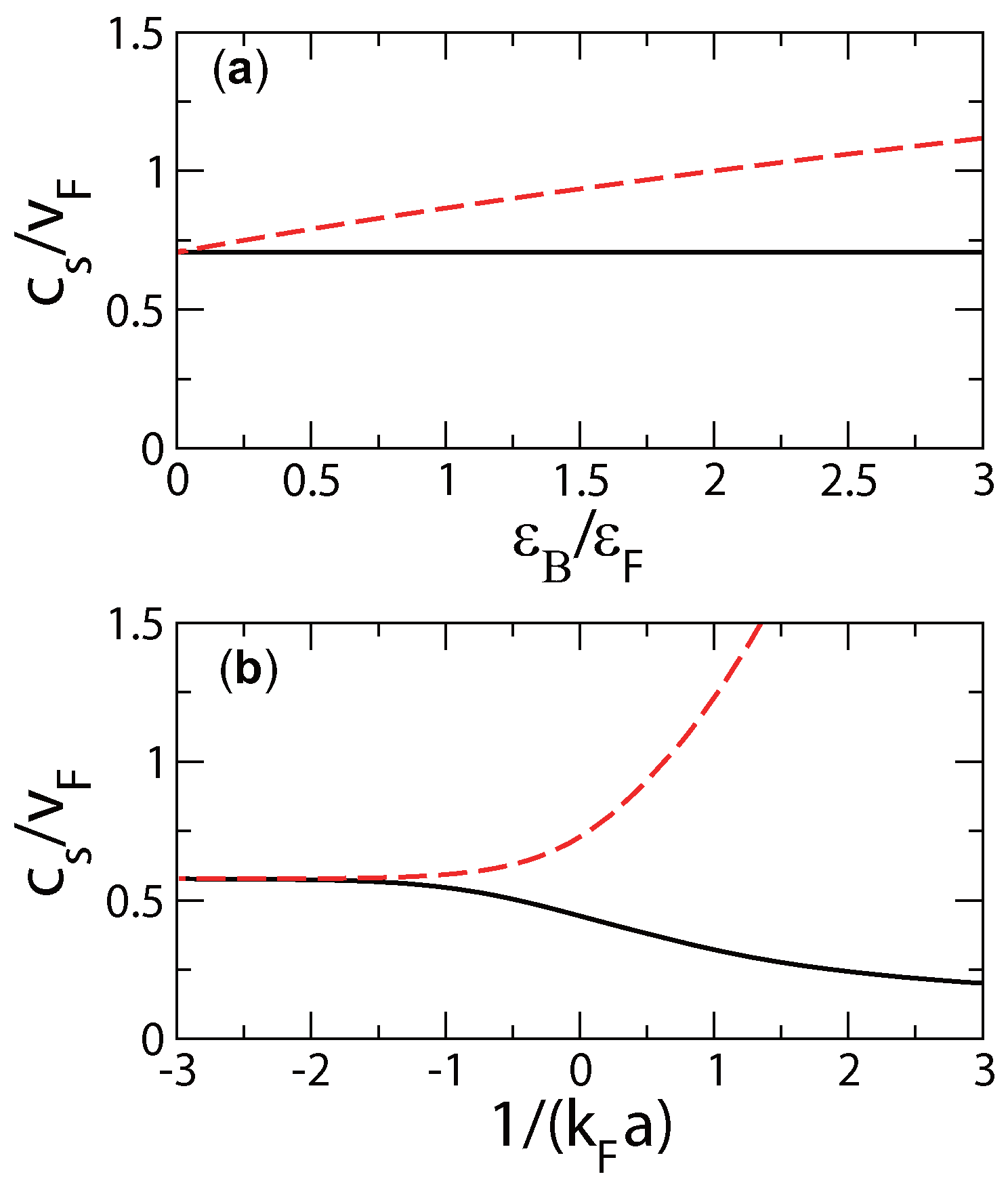
Figure 2.
First sound velocity in the 2D BCS–BEC crossover at zero temperature, calculated by using Equation (53). Here of the binding energy of the 2D Fermi superfluid and is the 2D Fermi energy. Dot-dashed line: obtained by using the mean-field number equation, Equation (45). Solid line: obtained by using the beyond-mean-field number equation, Equation (28).

Figure 3.
Adimensional pressure in the 2D BCS–BEC crossover, calculated using Gaussian pair fluctuation (GPF) theory (solid line) and using the Popov bosonic theory (dashed line). Experimental data (filled circles with error bars) are taken from [7]. is the pressure of the ideal 2D Fermi gas.
Figure 3.
Adimensional pressure in the 2D BCS–BEC crossover, calculated using Gaussian pair fluctuation (GPF) theory (solid line) and using the Popov bosonic theory (dashed line). Experimental data (filled circles with error bars) are taken from [7]. is the pressure of the ideal 2D Fermi gas.
© 2017 by the author. Licensee MDPI, Basel, Switzerland. This article is an open access article distributed under the terms and conditions of the Creative Commons Attribution (CC BY) license (http://creativecommons.org/licenses/by/4.0/).
Share and Cite
MDPI and ACS Style
Salasnich, L. Goldstone and Higgs Hydrodynamics in the BCS–BEC Crossover. Condens. Matter 2017, 2, 22. https://doi.org/10.3390/condmat2020022
AMA Style
Salasnich L. Goldstone and Higgs Hydrodynamics in the BCS–BEC Crossover. Condensed Matter. 2017; 2(2):22. https://doi.org/10.3390/condmat2020022
Chicago/Turabian StyleSalasnich, Luca. 2017. "Goldstone and Higgs Hydrodynamics in the BCS–BEC Crossover" Condensed Matter 2, no. 2: 22. https://doi.org/10.3390/condmat2020022