
Misconceptions about Calorimetry


1
Dipartimento di Fisica, Università di Pavia and INFN Sezione di Pavia, Via Bassi 6, Pavia 27100, Italy
2
Department of Physics, Texas Tech University, Lubbock, TX 79409-1051, USA
*
Author to whom correspondence should be addressed.
Instruments 2017, 1(1), 3; https://doi.org/10.3390/instruments1010003
Submission received: 29 March 2017
/
Revised: 2 May 2017
/
Accepted: 3 May 2017
/
Published: 10 May 2017
Abstract
:In the past 50 years, calorimeters have become the most important detectors in many particle physics experiments, especially experiments in colliding-beam accelerators at the energy frontier. In this paper, we describe and discuss a number of common misconceptions about these detectors, as well as the consequences of these misconceptions. We hope that it may serve as a useful source of information for young colleagues who want to familiarize themselves with these tricky instruments.
1. Introduction
In the past fifty years, calorimeters have become a very important component of the toolbox of particle physicists. Especially in experiments with large storage rings, where beams of high-energy particles are brought into collision with each other, calorimeter systems are the heart and soul of the detector system. Some of the reasons that make calorimeters extremely suitable for such experiments are
- The fact that they are sensitive to both the charged and neutral particles produced in the interactions.
- The fact that their performance typically improves with increasing energies.These two characteristics distinguish them from other detector components, which are typically only sensitive to charged particles and become less performant at increasing energy.
- The fact that they can provide the information needed for deciding whether a certain event is worth retaining for further (offline) inspection extremely fast. For example, in experiments at CERN’s Large Hadron Collider (LHC) proton-proton collisions take place at a rate of the order of 100 MHz. Yet, the calorimeter data make it possible to determine in real time which events should be saved.This is the most decisive reason for the important role of calorimeters in modern experiments, where the interesting events sometimes (i.e., at the LHC) represent a very tiny fraction of the total. The capability of calorimeter systems to provide information on the energy flow in the events (missing energy, transverse energy, jet production, etc.) is an extremely valuable feature in this context.
Despite the crucial role of calorimeters in many experiments, there are unfortunately still many misconceptions about these instruments. These misconceptions derive from the, in many ways, counter-intuitive performance characteristics. They have led and continue to lead to fundamental mistakes in designing detector systems, and interpreting results of experiments.
In this paper, we review a few common misconceptions, and describe some of the practical consequences. We mainly concentrate on sampling calorimeters, since that is where most of the problems occur. With few exceptions, most calorimeter systems at large experiments at colliders use indeed different materials for the absorption of the particles and for generating the signals resulting from this absorption process. Section 2 contains a brief introduction to calorimetry as a particle detection technique. In Section 3, the misconceptions and their consequences are described. In Section 4, we show how beam tests of prototype calorimeter modules are often at the origin of the problems. Conclusions and our outlook for the future are given in Section 5.
2. Calorimetry as a Particle Detection Technique
In nuclear and particle physics, the term calorimetry refers to the detection of particles, and measurement of their properties, through total absorption in an instrument called a calorimeter. Calorimeters exist in a wide variety, but they all have the common feature that the measurement process through which the particle properties are determined is destructive. Unlike, for example, wire chambers that measure a particle’s properties by tracking it in a magnetic field, the particles are no longer available for inspection by other devices once the calorimeter is done with them. One exception to this rule concerns muons. The fact that these particles may penetrate the substantial amount of matter represented by a calorimeter without losing much of their energy is actually an important ingredient for their identification as muons. Other particles (neutrinos and particles hypothesized in the context of Supersymmetry) typically do not leave any trace in a calorimeter, or in other detector components for that matter. Yet, calorimeters are also crucial tools for recognizing the presence of these particles, and measuring their properties.
In the absorption process, which is usually called shower development, almost all the particle’s energy is eventually converted into heat, hence the term calorimetry. However, the units of the energy involved in this process are typically very different from the thermodynamic ones. The most energetic particles in modern accelerator experiments are measured in units of TeV (1 TeV = eV = 1000 GeV), whereas 1 calorie (4.18 Joule) is equivalent to about TeV. The rise in temperature of the particle detector is thus, for all practical purposes, negligible, and therefore other ways to measure the deposited energy are employed. These methods are typically based on the measurable effects of atomic or molecular excitation (ionization charge, scintillation light), or on collective effects such as the production of Čerenkov light or sound in the absorbing medium.
2.1. Functions and Properties of Calorimeters
Calorimeters measure the energy released in the absorption of (sub)nuclear particles that enter them. They generate signals that make it possible to quantify that energy. Typically, these signals provide also other information about the particles, and about the event in which they were produced. The signals from a properly instrumented absorber may be used to measure the entire four-vector of the particles.
By analyzing the energy deposit pattern, the direction of the particle can be measured. The mass of the showering particle can be determined in a variety of ways, e.g., from the time structure of the signals, the energy deposit profile, or a comparison of the measured energy and momentum of the particle. Calorimeters are also used to identify muons and neutrinos. High-energy muons usually deposit only a small fraction of their energy in the calorimeter and produce signals in downstream detectors. Neutrinos typically do not interact at all in the calorimeter. If an energetic neutrino is produced in a colliding-beam experiment, this phenomenon will lead to an imbalance between the energies deposited in any two hemispheres into which a detector can be split. Such an imbalance is usually referred to as missing transverse energy.
The latter is an example of the energy flow information a calorimeter system can provide. Other examples of such information concern the total transverse energy and the production of hadronic jets in the measured events. Since this information is often directly related to the physics goals of the experiment, and since it can be obtained extremely fast, calorimeters usually play a crucial role in the trigger scheme, through which interesting events are selected and retained for further inspection off-line.
The calorimeter’s properties should be commensurate with the role it has to play in the experiment. Relevant properties in this context are the energy resolution, the size (which determines the effects of shower leakage), the signal speed and the hermeticity.
2.2. Calorimeter Types
One frequently distinguishes between homogeneous and sampling calorimeters. In a homogeneous calorimeter, the entire detector volume is sensitive to the particles and may contribute to the generated signals. In a sampling calorimeter, the functions of particle absorption and signal generation are exercised by different materials, called the passive and active medium, respectively. The passive medium is usually a high-density material, such as iron, copper, lead or uranium. The active medium generates the light or charge that forms the basis for the signals from such a calorimeter.
In some non-accelerator experiments, the calorimeter is also the source that generates the particles to be detected. As examples, we mention large water Čerenkov counters built to detect astrophysical neutrinos and the high-purity 76Ge crystals or the 136Xe liquid used to study decay.
2.2.1. Electromagnetic Calorimeters
Electromagnetic calorimeters are specifically intended for the detection of energetic electrons and s, but produce usually also signals when traversed by other types of particles. They are used over a very wide energy range, from the semiconductor crystals that measure X-rays down to a few keV to shower counters such as AGILE, PAMELA and FERMI, which orbit the Earth on satellites in search for electrons, positrons and s with energies >10 TeV. These calorimeters don’t need to be very massive, especially when high-Z absorber material is used. For example, when 100 GeV electrons enter a block of lead, ∼90% of their energy is deposited in only 4 kg of material. By far the best energy resolutions have been obtained with large semiconductor crystals, and in particular high-purity germanium. These are the detectors of choice in nuclear ray spectroscopy, and routinely obtain resolutions () of 0.1% in the 1 MeV energy range. The next best class of detectors are scintillating crystals, which are often the detectors of choice in experiments involving rays in the energy range from 1–20 GeV, which they measure with energy resolutions of the order of 1%. Excellent performance in this energy range has also been reported for liquid krypton and xenon detectors, which are bright (UV) scintillators. Other homogeneous detectors of em showers are based on Čerenkov light, in particular lead glass. Very large water Čerenkov calorimeters (e.g., SuperKamiokande) should also be mentioned in this category.
Sampling calorimeters, which are typically much cheaper, become competitive at higher energies. In properly designed instruments of this type, the energy resolution is determined by sampling fluctuations. These represent fluctuations in the number of different shower particles that contribute to the calorimeter signals, convoluted with fluctuations in the amount of energy deposited by individual shower particles in the active calorimeter layers. They depend both on the sampling fraction, which is determined by the ratio of active and passive material, and on the sampling frequency, determined by the number of different sampling elements in the region where the showers develop. Sampling fluctuations are stochastic and their contribution to the energy resolution is described by [1]
in which d represents the thickness of individual active sampling layers (in mm), and the sampling fraction for minimum ionizing particles (mips). This expression describes data obtained with a large variety of different (non-gaseous) sampling calorimeters reasonably well.
2.2.2. Hadron Calorimeters
The energy range covered by hadron calorimeters is in principle even larger than that for em ones. Calorimetric techniques are used to detect thermal neutrons, which have kinetic energies of a small fraction of 1 eV, to the highest-energy particles observed in nature, which reach the Earth from outer space as cosmic rays carrying up to eV or more. In accelerator-based particle physics experiments, hadron calorimeters are typically used to detect protons, pions, kaons and fragmenting quarks and gluons (commonly referred to as jets) with energies in the GeV-TeV range. In this paper, we mainly discuss the latter instruments.
The development of hadronic cascades in dense matter differs in essential ways from that of electromagnetic ones, with important consequences for calorimetry. Hadron showers consist of two distinctly different components:
- An electromagnetic component; s and s generated in the absorption process decay into s which develop em showers.
- A non-electromagnetic component, which combines essentially everything else that takes place in the absorption process.
For the purpose of calorimetry, the main difference between these components is that some fraction of the energy contained in the non-em component does not contribute to the signals. This invisible energy, which mainly consists of the binding energy of nucleons released in the numerous nuclear reactions, may represent up to 40% of the total non-em energy, with large event-to-event fluctuations.
The appropriate length scale of hadronic showers is the nuclear interaction length (), which is typically much larger (up to 30 times for high-Z materials) than the radiation length (), which governs the development of em showers. Many experiments make use of this fact to distinguish between electrons and hadrons on the basis of the energy deposit profile in their calorimeter system. Since the ratio is proportional to Z, particle identification on this basis works best for high-Z absorber materials. Lead and depleted uranium are therefore popular choices for the absorber material in preshower detectors and the first section of a longitudinally segmented calorimeter, which is therefore commonly referred to as the electromagnetic section.
Just as for the detection of em showers, high-resolution hadron calorimetry requires an average longitudinal containment better than 99%. In iron and materials with similar Z, which are most frequently used for hadron calorimeters, 99% longitudinal containment requires a thickness ranging from at 20 GeV to at 150 GeV. Hadronic energy resolutions of 1% require not only longitudinal shower containment at the 99% level, but also lateral containment of 98% or better.
Energetic s may be produced throughout the absorber volume, and not exclusively in the em calorimeter section. They lead to local regions of highly concentrated energy deposit. Therefore, there is no such thing as a “typical hadronic shower profile”. This feature affects not only the shower containment requirements, but also the calibration of longitudinally segmented calorimeters in which one tries to improve the quality of calorimetric energy measurements of jets with an upstream tracker, which can measure the momenta of the charged jet constituents with great precision. This method has become known as Particle Flow Analysis (PFA).
2.2.3. Compensation
The properties of the em shower component have also important consequences for the energy resolution, the signal linearity and the response function. The average fraction of the total shower energy contained in the em component has been measured to increase with energy following a power law:
where is a material dependent constant related to the average multiplicity in hadronic interactions (varying from 0.7 GeV to 1.3 GeV for -induced reactions on Cu and Pb, respectively), and . For proton-induced reactions, is typically considerably smaller, as a result of baryon number conservation in the shower development.
Let us define the calorimeter response as the conversion efficiency from deposited energy to generated signal, and normalize it to electrons. The responses of a given calorimeter to the em and non-em hadronic shower components, e and h, are usually not the same, as a result of invisible energy and a variety of other effects. Such calorimeters are called non-compensating (). Since their response to hadrons, , is energy dependent (2), they are intrinsically non-linear.
Event-to-event fluctuations in are large and non-Poissonian. If , these fluctuations tend to dominate the hadronic energy resolution and their asymmetric distribution characteristics are reflected in the response function. The effects of non-compensation on resolution, linearity and line shape, as well as the associated calibration problems [2] are absent in compensating calorimeters (). Compensation can be achieved in sampling calorimeters with high-Z absorber material and hydrogenous active material. It requires a very specific sampling fraction, so that the response to shower neutrons is boosted by the precise factor needed to equalize e and h. For example, in Pb/scintillating-plastic structures, this sampling fraction is ∼2% for showers [3,4,5]. This small sampling fraction sets a lower limit on the contribution of sampling fluctuations, while the need to efficiently detect MeV-type neutrons requires signal integration over a relatively large volume during at least 30 ns. Yet, calorimeters of this type currently hold the world record for hadronic energy resolution (/E ∼30%/ [4]).
Excellent hadronic performance has also been achieved with calorimeters that use the dual-readout method (DREAM) [6]. Such calorimeters produce two signals that provide complementary information about the shower development. Since Čerenkov light is almost exclusively produced in the em shower component, a comparison of the Čerenkov signal with a signal to which all charged shower particles contribute, the value of can be measured for each individual event. This makes it possible to eliminate the detrimental effects of fluctuations in this variable and achieve similar performance as intrinsically compensating calorimeters, without the mentioned disadvantages.
3. Common Misconceptions and Their Consequences
3.1. Shower Particles Contributing to the Calorimeter Signals
The most common, important and consequential misconception about calorimetry is that a shower is a collection of minimum ionizing particles (mips). Already in the early days, it was realized that the signal from a high-energy electron absorbed in a sampling calorimeter was substantially different from that of a muon that traversed this calorimeter and deposited the same energy in it as the showering electron. This is due to the fact that the composition of the em shower changes as a function of depth, or age.
In the late stages, most of the energy is deposited by soft s which undergo Compton scattering or photoelectric absorption, and the sampling fraction for this shower component (i.e., the fraction of the energy that contributes to the calorimeter signals) may be very different from that of the mips that dominate the early stages of the shower development. This causes major complications for the intercalibration of the different sections of a longitudinally segmented calorimeter, as is well known from the experiences of several experiments that have had to deal with this problem [11,12].
3.1.1. Intercalibration Problems
Figure 1 illustrates how the sampling fraction of a given calorimeter structure depends on the stage of the developing showers. In calorimeters consisting of high-Z absorber material (e.g., lead) and low-Z active material (plastic, liquid argon), the sampling fraction may vary by as much as 25%–30% over the volume in which the absorption takes place [13]. An example of the pitfalls that this causes for calibrating a longitudinally segmented device concerns the calorimeter for the AMS-02 experiment at the International Space Station [12]. This calorimeter has eighteen independent longitudinal depth segments. Each layer consists of a lead absorber structure in which large numbers of plastic scintillating fibers are embedded, and is about thick. A minimum ionizing particle deposits 11.7 MeV upon traversing such a layer. The AMS-02 collaboration initially calibrated this calorimeter by sending muons through it and equalizing the signals from all eighteen longitudinal segments. This seems like a very good method to calibrate this detector, since all layers have exactly the same structure.
However, when this calorimeter module was exposed to beams of high energy electrons, it turned out to be highly non-trivial how to reconstruct the energy of these electrons. Figure 2a shows the average signals from 20 GeV electron showers developing in this calorimeter. These signals were translated into energy deposits based on the described calibration. The measured data were then fitted to a -function and since the showers were not fully contained, the average leakage was estimated by extrapolating this fit to infinity. As shown in Figure 2b, this procedure systematically underestimated this leakage fraction, more so as the energy (and thus the leakage) increased. The reason for this is that a procedure in which the relationship between measured signals and the corresponding deposited energy is assumed to be the same for each depth segment will cause the energy leakage to be systematically underestimated, more so if that leakage increases.
This very complicated problem will most definitely also affect calorimeters based on Particle Flow Analysis (PFA) [14], which are all based on structures that are highly segmented, both longitudinally and laterally. The underlying problem is that the relationship between deposited energy and resulting signal is not constant throughout a developing shower. As the composition of the shower changes, so does the sampling fraction. Figure 2 provides a clear example of the problems that this may cause.
3.1.2. Catastrophic Effects
Another aspect of the misconception that a shower is a collection of mips is the fact that a single shower particle may cause catastrophic effects for the calorimeter performance. This is particularly true for hadron showers, and may be illustrated by a recent example taken from the CMS experiment. The CMS calorimeter system consists of a crystal based em calorimeter, followed by a brass/plastic-scintillator hadronic compartment. Each PbWO4 crystal is read out by two Avalanche Photo Diodes (APDs, Figure 3a).
When hadrons are sent into this calorimeter system, it sometimes produces events in which an anomalously large signal is recorded in one individual crystal [15]. Such events are referred to as “spikes” (Figure 3b). Figure 3c shows an example of a nuclear interaction that is a typical feature in hadron shower development. A proton with a momentum of 0.57 GeV/c interacts with a nucleus of the absorber structure, and produces seven even lower-energy charged particles, presumably protons and/or nuclear aggregates such as particles in this process. There are probably also at least as many neutrons produced in this reaction, but these do not ionize the material and are thus invisible in this figure. The charged fragments are all heavily ionizing, with typical values of 100–1000 times that of a mip. If such an event happens close to an APD, these charged fragments may create a very large signal. The APDs are intended to detect scintillation photons produced in the PbWO4 crystals, and the energy scale of the calorimeter signals is set by the production rate of such photons. However, the APDs produce signals that are orders of magnitude larger when traversed by a charged particle. The densely ionizing fragments of an event such as the one shown in Figure 3c may produce signals that are interpreted as an energy deposit of several hundred GeV inside the scintillating crystals, and this is precisely what causes these spikes. As an aside, we mention that this phenomenon should be very easily recognizable if the two APDs connected to each crystal were read out separately, since the described phenomenon would only occur in one of them. However, in order to save money, CMS had ganged them together and treated the two APDs as one readout cell.
After having realized the value of redundant detector information the hard way, CMS has decided to modify the readout of another component of its calorimeter system (HF, intended to detect particles produced at very small angles with the bean line) with a system in which several photon detectors independently measure the light produced in a given calorimeter tower. In this way, background induced by beam halo particles in individual light detectors could be reduced [16].
Another well known example of a catastrophic effect caused by a single shower particle occurs in sampling calorimeters with gaseous active media, such as proportional wire chambers that use a gas mixture containing free hydrogen atoms, e.g., isobutane. Neutrons, which are abundantly produced in hadronic shower development, may elastically scatter off a hydrogen nucleus and the recoil proton may be stopped in the wire chamber. The result is a signal contribution that may be orders of magnitude larger than the signal from a mip traversing the wire chamber. Because of the extremely small sampling fraction of such calorimeters (typically ∼, a 1 MeV energy deposit by a recoil proton is thus interpreted as a 100 GeV energy deposit in the calorimeter. This phenomenon became known as the “Texas Tower effect” in CDF [17] and necessitated a complete replacement of the forward calorimeter system in that experiment.
3.2. Signal (Non)linearity
Calorimeters may be non-linear for a variety of reasons. Intercalibration of longitudinal sections, signal saturation and the energy dependence of the em shower fraction (in hadron showers) are the most common causes. Many calorimeters are non-linear, even though their owners sometimes pretend otherwise.
A common misconception is that a calorimeter is linear if the average signals plotted versus the deposited energy can be described with a straight line. This is not what is meant by a linear calorimeter. The straight line has to extrapolate through the origin of the plot. Signal linearity means that the average calorimeter signal is proportional to the deposited energy, i.e., the response is constant.
Figure 4 illustrates this issue. The experimental data were obtained with a W/Si em calorimeter built by CALICE [18]. The authors fit the measured signals with the following expression:
Then, they define
and plot
as a function of the beam energy. The result is represented by the (black) squares in Figure 4b. They conclude that “the calorimeter is linear to within approximately 1%”. This is highly misleading. When the calorimeter signals they actually measured are used to check the linearity, i.e., when
is plotted as a function of the beam energy, the results, represented by the (red) full circles in Figure 4b, look quite different. We conclude from these results that the authors measured a signal non-linearity of 5% over one decade in energy.
3.2.1. Non-Linearity Resulting from Signal Saturation
Whereas the non-linearity discussed in the previous subsection is probably the result of the intercalibration of the numerous longitudinal segments of this PFA calorimeter, Figure 5 shows non-linearity with a different origin. It concerns data obtained with a digital hadron calorimeter built by CALICE [14]. This calorimeter contains 500,000 readout cells ( cm2 RPCs), which produce “digital” signals (“yes” or “no”) in response to charged particles. However, this type of cell produces the same signal, regardless whether it is caused by 1, 3 or 29 shower particles. This leads to signal non-linearity, especially in em showers. Since the lateral shower profile is independent of the energy of the showering particle, and the longitudinal shower profile only varies logarithmically with that energy, the density of shower particles in the region where the energy is deposited increases almost proportionally with the shower energy, signal non-linearity is inevitable. The same is true for hadron showers, albeit that the shower particle density is smaller in that case, and the non-linearity effects correspondingly less pronounced.
We use data from one of our own experiments to illustrate the effects of signal saturation. The SPACAL calorimeter (Figure 6a) consisted of 155 hexagonal towers. Each of these towers was calibrated by sending a beam of 40 GeV electrons into its geometric center. Typically, 95% of the shower energy was deposited in that tower, and the remaining 5% was shared among the six neighbors. The high-voltage settings were chosen such that the maximum energy deposited in each tower during the envisaged beam tests would be well within the dynamic range of that tower. For most of the towers (except the central septet), the dynamic range was chosen to be 60 GeV.
When we did an energy scan with electrons in one of these non-central towers, the results shown in Figure 6b and c were obtained. Up to 60 GeV, the average calorimeter signal increased proportionally with the beam energy, but above 60 GeV, a non-linearity became immediately apparent (Figure 6b). The signal in the targeted tower had reached its maximum value, and would from that point onward produce the same value for every event. Any increase in the total signal was due to the tails of the shower, which developed in the neighboring towers. A similar trend occurred for the energy resolution (Figure 6c). Beyond 60 GeV, the energy resolution suddenly improved dramatically. Again, this was a result of the fact that the signal in the targeted tower was the same for all events at these higher energies. The energy resolution was thus completely determined by event-to-event fluctuations in the energy deposited in the neighboring towers by the shower tails.
A similar situation occurred in the CALICE calorimeter of which the results are shown in Figure 5. And since also in this calorimeter an important source of fluctuations is suppressed, the energy resolution measured with it is meaningless. We should emphasize that the described effects may in practice be less obvious, especially in more complicated setups and for complex events.
3.2.2. Non-Linearity for Hadron Detection
Calorimeters intended for the detection of hadron showers are typically intrinsically non-linear, as a result of the fact that the average em shower fraction depends on the energy of the showering particle. Non-compensating calorimeters respond differently to the em and non-em shower components (), and the overall calorimeter response reflects the fact that the energy sharing between these shower components is energy dependent. These signal non-linearities for hadron detection are thus the result of the physics of the shower development process, they do not depend on peculiarities of the calorimeter signals, as in the examples described in the previous subsection. For that reason, hadronic signal non-linearity does in general not preclude an (on average) correct measurement of the energy of the showering particle on the basis of the observed signals. This is not necessarily true for all the non-linearities that may affect electromagnetic shower detection, such as the ones discussed in the next subsection.
A (on average) correct measurement of hadronic energy deposits is possible, provided that the em energy scale has been determined in the same way for all longitudinal calorimeter segments. In that case the hadronic response can be determined with hadron beams of different energy, using the em energy scale. An example is shown in Figure 7. The correct hadron energy is then found by multiplying the measured energy with the inverse of the calorimeter response for that energy. The figure shows slightly different responses for different types of hadrons, but in CMS this is a secondary effect compared to the large dependence of the response on the starting point of the showers [19].
3.2.3. Signal Non-Linearity as a Result of Miscalibration
One of the most common reasons for signal non-linearity is the method chosen to intercalibrate the various longitudinal sections of a longitudinally segmented calorimeter. This is illustrated with the example of the HELIOS calorimeter [20], discussed below. This calorimeter consisted of two longitudinal segments, with depths of and 4 , respectively (Figure 8a). Electrons developing in this structure deposited comparable amounts of energy in each section, but the precise energy sharing depended on the energy of the showering particle. The intercalibration of the signals from the two sections was performed by minimizing the width of the total signal distribution. Figure 8b shows how this width depended on the choice of the ratio of the calibration constants for the signals from both sections, . The optimum value turned out to be different from the value for muons. The latter could simply be calculated from the composition of the two sections.
If we take for muons, then the optimal value for electrons was around 0.6–0.9, depending on the energy. This can be understood from the fact that the sampling fraction decreased as the shower developed (Figure 1). Since the sampling fraction in the first section was larger, a smaller total width was obtained when signals from that section were attributed a relatively larger weight, hence the optimal value . Now, if the electron energy increases, a larger fraction of that energy is deposited in the second calorimeter section. And since the signals from that section are given a relatively small weight, the result is a total signal that is smaller than if the signals from both sections had been given the same weights as mips (). In other words, the calorimeter response (i.e., the average signal per GeV) decreases.
A calibration procedure in which the width of the total signal distribution of showers that develop in several different calorimeter segments is minimized thus leads inevitably to a non-linear response. Now one might argue that there is in principle no reason why a calorimeter that is non-linear for electromagnetic shower detection, although somewhat inconvenient, should be unacceptable. After all, all non-compensating calorimeters are intrinsically non-linear for hadron and jet detection and one uses those too, in many experiments.
Any type of non-linearity could in principle be dealt with by means of a polynomial relationship between the signals S and the corresponding energy E:
and the fact that other constants than have a non-zero value might be a small price to pay for improving energy resolution.
This line of reasoning is, however, crucially flawed [21]. The non-linearity introduced by this weighting scheme implies by definition that a high-energy , decaying into two unresolved s produces, on average, a larger signal in this calorimeter than an electron, or one photon, of the same energy. An resonance decaying into three unresolved s produces an even larger signal, and an energetic decaying into , or even tops them all (Figure 8d). By introducing a signal non-linearity, the calorimeter response is made dependent on such differences. And since, in practice, the calorimeter information does not always allow one to tell whether the signal was caused by one, two, three or even more s, the systematic differences in the average calorimeter response for those cases are an integral part of the energy resolution. Interpreting the width of the signal distribution measured for single electrons from a test beam as the em energy resolution is thus incorrect.
The approach chosen in this case (minimization of the width of the total signal distribution) is only one of several different methods described in the literature for intercalibrating the different sections of a longitudinally segmented calorimeter. Other methods aim to achieve
- Correct energy reconstruction of pions penetrating the electromagnetic compartment without starting a shower, or
- Hadronic signal linearity, or
- Independence of hadron response on starting point shower, or
- Equal response to electrons and pions.
Each of these approaches introduces specific additional problems [22]. Intercalibrating the different sections of a longitudinally segmented calorimeter system is in practice one of the most daunting tasks when commissioning a detector, and it is fundamentally impossible to achieve a result in which the signals measured in the different sections can be correctly translated into deposited energy. This is even true for compensating calorimeters. The combination of the energy dependence of the shower profiles, combined with the depth dependence of the sampling fraction are responsible for this problem.
The best way to intercalibrate the different sections of a longitudinally segmented calorimeter system is by using the same particles for all individual sections. If these particles develop showers, then they can only be used to calibrate sections in which these showers are completely contained. Only in this way is the relationship between the deposited shower energy (in GeV) and the charge (in picoCoulombs) generated as a result established unambiguously. We have referred to this as the method. The use of a beam of muons to intercalibrate the eighteen segments of the AMS-02 electromagnetic calorimeter (Figure 2) definitely qualifies as a viable method in this respect. The mistake made in that case did not concern the calibration method itself, but the interpretation of the results.
3.3. Energy Resolution
A common mistake with regards to energy resolution has to do with its very definition. The energy resolution is the precision with which the energy of an unknown object can be determined from the signals it produces in the calorimeter. Typically, this resolution is determined as the relative width of the signal distribution measured for a beam of mono-energetic particles from an accelerator. However, this is only correct if the average value of that measured signal distribution corresponds indeed to the correct energy of these particles. Response non-linearities tend to invalidate that assumption, as illustrated by the example shown in Figure 8d.
Often, the measured signal distributions exhibit non-Gaussian tails. In that case, one should quote the value as the energy resolution. However, some authors use another variable, in order to make the results less dependent on the tails of the signal distributions they measure, and thus look better. This variable, called , is defined as the root-mean-square of the energies located in the smallest range of reconstructed energies which contains 90% of the total event sample. For the record, it should be pointed out that for a perfectly Gaussian distribution, this variable gives a 21% smaller value than the true (i.e., ). Of course, one is free to define variables as one likes. However, one should then not use the term “energy resolution” for the results obtained in this way, and compare results obtained in terms of with genuine energy resolutions from calorimeters with Gaussian response functions [23]. This misleading practice is generally followed by the proponents of PFA.
Another widespread misconception concerns the way in which the energy resolution of a calorimeter is quoted. Frequently, the relative energy resolution () of a particular calorimeter is expressed as . However, this is rarely a correct description of reality, since in practice other factors, which are not governed by Poisson statistics, contribute to the energy resolution, and such factors often dominate the performance, especially at the low and high ends of the energy spectrum for which the detector is intended.
As an example, Figure 9 shows the hadronic energy resolutions of the ZEUS and the ATLAS calorimeters. The experimental data points are plotted on a scale that is linear in and runs from right to left. Scaling with implies that the data points should be located on a straight line through the bottom right corner in this plot. This is indeed the case for the compensating ZEUS calorimeter, for which the resolution is quoted as . However, the resolution of ATLAS does not at all scale with . As a matter of fact, the data points are at all energies located well above the line in this plot, and for energies larger than 100 GeV, the resolution is more than a factor of four worse than for ZEUS. Yet, in talks about ATLAS, the hadronic energy resolution is often quoted as .
Another mistake that is not uncommon concerns the extrapolation of measurement results far beyond their region of validity, We mention two examples.
The HELIOS Collaboration measured a resolution for 3.2 TeV 16O ions [20], and the WA80 Collaboration, which also operated a uranium/scintillator calorimeter, found a resolution of 1.7% for 6.4 TeV 32S ions [26]. One should realize, however, that in these cases a convolution of either 16 or 32 independent 200 GeV nucleon showers was measured. Hence, strictly speaking, these results only say something about the precision of the energy measurement for a 200 GeV nucleon shower. If sixteen signals from such showers are convolved, then the resulting signal has a resolution that is four (= ) times smaller than the resolution for the individual signals from 200 GeV nucleons. In other words, if the resolution for 200 GeV protons (or neutrons) was 7.6%, then a resolution of 1.9% should be expected for 16O ions with an energy of 3.2 TeV. The measured resolution for heavy ions at multi-TeV energies is thus by no means indicative for the resolution that may be expected for the detection of single hadrons or jets carrying such energies.
A similar statement should be made concerning the “determination” of the energy resolution for high-energy electromagnetic shower detection in liquid xenon, based on convolving the signals from large numbers of low-energy electrons (100 keV) recorded in a small cell [27]. Also in this case, the measurements only revealed something about the energy resolution for the detection of these low-energy electrons. In a high-energy em shower, a variety of new effects, absent or negligible in the case of these electrons, affect the signals and their fluctuations. As an example of such effects, we mention the fact that the (174 nm) shower light is produced in a large detector volume. Light attenuation, e.g., through self-absorption and shower leakage, are the likely consequences of this.
These examples illustrate that, in general, measurements made for low-energy particles cannot be used to determine/predict the high-energy calorimeter performance.
Finally, we want to point out that often times a good energy resolution is only part of the requirements for obtaining the desired physics sensitivity. As an example, we mention the Higgs boson, discovered in 2012 by two experiments at the Large Hadron Collider through its decay mode [28,29]. The invariant mass of a particle decaying into two s is given by
The precision with which the mass can be measured is thus not only determined by the energy resolution, i.e., the measurement uncertainty on the energies and , but also by the relative uncertainty on the angle () between the directions of these s. A good localization of the s is thus very important to identify the parent particle. While CMS emphasized excellent energy resolution for em showers in its design of the experiment, at the expense of degraded hadronic performance, ATLAS concentrated its efforts also on the localization issue. As a result, the mass resolution for the Higgs bosons turned out to be very similar in both experiments.
3.4. Effects of Non-Compensation
Almost all calorimeters that are operating in large storage ring experiments are non-compensating. This means that the responses (i.e., the average signal per unit deposited energy) to the em and non-em components of hadron showers are not the same in these calorimeters (). The consequences of this feature are a source of several misconceptions. Often, an additional constant term in the hadronic energy resolution is considered the main, if not the only, consequence of non-compensation. This is a misconception at several levels. Not only is non-compensation the cause of a number of other serious problems, but the effect on the hadronic energy resolution is by no means independent of energy, as suggested by the concept of an additional constant term.
The incorrectness of this notion is illustrated by the fact that the hadronic energy resolution of non-compensating calorimeters is not only considerably worse compared to compensating ones at high energies, but also at low energies. The resolution of the best hadron calorimeters, such as the one used for the ZEUS experiment [24], is ∼30%/, i.e., at 10 GeV (Figure 9). Adding a constant term of 5% (in quadrature) would increase this resolution to ∼11%. However, the energy resolution of non-compensating calorimeters is typically two to three times larger at this energy. The effects of non-compensation are thus by no means limited to high energy, where a constant term tends to dominate the contributions that are determined by Poisson fluctuations.
The correct way of incorporating the effects of non-compensation on the hadronic energy resolution is given by Equation (7), and illustrated in Figure 10.
The effects are described by an energy dependent term, added in quadrature to the scaling term that accounts for the Poisson fluctuations ( in this example). The coefficient of this non-compensation term, in this example, is determined by the degree of non-compensation: , and [30].
Figure 10 also shows that the correct description of the hadronic energy resolution yields in practice almost identical results as an expression in which a constant term () is added linearly to a scaling term (). There are several examples in the literature in which such an expression is used to describe the hadronic energy resolution. However, the linear addition of two terms suggests complete correlation between the effects described by these terms, which is nonsense in this situation. Figure 10 shows that one has to go to very high energies, beyond the reach of the current generation of available test beams, to see a significant difference between the two mentioned expressions. However, only one of these expressions (the red one) is correct, and indicates that the effects of non-compensation on the hadronic energy resolution are indeed energy dependent.
However, a hadronic energy resolution that deviates from scaling is not the only consequence of non-compensation. Among the other effects, we mention
- Hadronic signal non-linearity (see Section 2.2.2). This is a result of the fact that the average em fraction of hadron showers, , increases with energy.
- Non-Gaussian response functions. This is a consequence of the fact that the distribution of is not Gaussian, but asymmetric, favoring large values (Figure 11).This may cause problems, such as trigger biases. For example, if one uses the calorimeter signals to select events with a minimum (missing) transverse energy from a steeply falling distribution, then the event sample is likely to be strongly dominated by events in which the actual value of this energy was smaller than the trigger level, but in which upward fluctuations pushed it beyond that level. An asymmetric response function makes it very difficult to deal with this problem in a correct way.
- Different response functions for different hadrons (protons, pions, kaons) of the same energy. This is the topic of the next subsection.
3.5. Particle Dependence of the Calorimeter Response
The absorption of different types of hadrons in a calorimeter may differ in very fundamental ways, as a result of applicable conservation rules. For example, in interactions induced by a proton or neutron, conservation of baryon number has important consequences. The same is true for strangeness conservation in the absorption of kaons. This has implications for the way in which the shower develops. For example, in the first interaction of a proton, the leading particle has to be a baryon. This precludes the production of an energetic which carries away most of the proton’s energy. Similar considerations apply in the absorption of strange particles. On the other hand, in pion-induced showers it is not at all uncommon that most of the energy carried by the incoming particle is transferred to a . The resulting shower is in that case almost completely electromagnetic. This phenomenon is the reason for the asymmetric distributions from Figure 11.
Experimental studies have confirmed these effects. Figure 12 shows the signal distributions measured for 300 GeV pions (a) and protons (b), respectively. The signal distribution for protons is much more symmetric, as indicated by the Gaussian fit. This is because the em component of proton-induced showers is typically populated by s that share the energy contained in this component more evenly than in pion-induced showers.The figure also shows that the rms width of the proton signal distribution is significantly smaller (by ∼20%) than for the pions. Figure 12c shows that the average signal per GeV deposited energy is smaller for the protons than for the pions, by about 10%. This is also a consequence of the limitations on production that affect the proton signals in this non-compensating calorimeter (). So while the response to protons is smaller in this calorimeter, the energy resolution is better. Similar effects are expected to play a role for the detection of kaons, where production is limited as a result of strangeness conservation in the shower development.
Whereas the phenomena discussed above are the result of differences in the electromagnetic shower component, which lead to differences in the response functions of the calorimeter to baryons, pions and kaons, other effects may also cause significant differences that at first sight might be unexpected. As an example, we mention the differences between electron and photon detection in a calorimeter. These are important, since the electromagnetic performance is typically experimentally studied with electron beams, whereas photon detection may be the most important goal1. Showers initiated by high-energy photons and electrons are quite different in the early stage of the absorption process, before the shower maximum [21].
- Photon-induced showers deposit their energy, on average, deeper inside the absorbing structure than do em showers induced by charged particles of the same energy. The response differences in Figure 8d are the result of this.
- The fluctuations in the amount of energy deposited in a given slab of material are larger for showers induced by photons than for showers induced by or .
The first effect results from the fact that the photons travel a certain distance (9/7 , on average) in the absorbing structure before they start losing energy, while electrons and positrons start losing energy immediately upon their entry. Moreover, the starting point of the photon-induced showers fluctuates from event to event, which leads to the second effect.
These effects are illustrated in Figure 13, which shows the distribution of the energy deposited by 10 GeV electrons and 10 GeV photons in a (2.8 cm) thick slab of lead. On average, the electrons deposit more energy in this material than the photons (2.10 GeV vs.1.48 GeV). However, the fluctuations in the energy deposited by the photons are clearly larger than those in the energy deposited by the electrons (0.86 GeV vs.0.64 GeV). The distribution for the photon showers exhibits an excess near zero, which is the result of photons penetrating (almost) the entire slab without interacting. The “punch-thru” probability for a high-energy is in this example .
The different effects of dead material installed in front of the calorimeter on electrons/positrons and s is relevant for experiments such as ATLAS, where the electromagnetic calorimeter is “hidden” in a cryostat, although the fact that this cryostat is made of aluminium makes the effects less dramatic than suggested in Figure 13. Another consequence of the differences between electron and induced showers is the fact that the very complicated calibration scheme that was developed for electrons showering in the three longitudinal segments of the ATLAS ECAL [11] is not necessarily the optimal solution for detection in this calorimeter.
3.6. The Perceived Benefits of Longitudinal Segmentation
There is a deeply rooted belief that calorimeter systems for high-energy collider experiments should be longitudinally subdivided into several sections. As a minimum, one will usually want to have an electromagnetic and a hadronic section. A major reason for this belief is that such a subdivision is needed for recognizing em showers, and thus identify electrons and s entering the calorimeter.
This is a myth. It has been demonstrated repeatedly that there are several ways to identify em showers in longitudinally unsegmented calorimeters. For example, the DREAM Collaboration has demonstrated four different methods that can be used to achieve this [33]. These methods are based on
- The measured lateral shower profile,
- A comparison between the scintillation and Čerenkov signals produced by the developing shower,
- The time structure of the signals, and in particular the starting time of the signals with respect to the signal produced in an upstream detector, or the pulse width.
Figure 14 illustrates one of these methods, which is based on the starting time of the calorimeter signals, measured with respect to the signal produced by an upstream detector. This method is based on the fact that the light in the optical fibers travels at a lower speed than the particles that generate this light. The deeper inside the calorimeter the light is produced, the earlier the calorimeter signal starts. For the polystyrene fibers, the effect amounted to 2.55 ns/m. For the tested calorimeter, this led to a longitudinal position resolution of ∼20 cm.
Figure 14 shows the measured distribution of the starting time of the signals from 60 GeV (Figure 14a) and (Figure 14b). This pion distribution peaked ∼1.5 ns earlier than that of the electrons, which means that the light was, on average, produced 60 cm deeper inside the calorimeter. The distribution is also asymmetric, it has an exponential tail towards early starting times, i.e., light production deep inside the calorimeter. This signal distribution was also used to reconstruct the average depth at which the light was produced for individual pion showers. The result, depicted in Figure 14c, essentially shows the longitudinal profile of the 60 GeV pion showers in this calorimeter.
It was shown in this paper that by combining all the available methods, which in several different ways exploited complementary information about the events, the longitudinally unsegmented RD52 fiber calorimeter could be used to identify electrons with a very high degree of accuracy. Using the time structure of the signals, the lateral shower profile and a comparison of the Čerenkov and scintillation signals, more than 99% of the electrons entering the detector were correctly identified with criteria that ruled out almost all hadronic particles as electron candidates. In practice, this is probably somewhat too optimistic, because of difficulties encountered in more realistic conditions than beam tests of prototype modules.
However, good electron/pion separation can already be achieved with much less sophisticated methods. Especially in beam tests, a very simple preshower detector (PSD), placed in front of the calorimeter, may do an adequate job. Such a device may consist of a plate of lead, 1 cm (1.9, 0.06) thick, followed by a sheet of plastic scintillator. When a beam consisting of a mixture of high-energy electrons and pions is sent through this device, almost all pions (96%) traverse it without strongly interacting. These pions produce a minimum ionizing peak in the scintillator. On the other hand, the electrons lose a considerable fraction of their energy by radiating large numbers of bremsstrahlung photons. Some of these photons convert into pairs in the PSD and thus contribute to the scintillation signals produced by this device.
The result is a very clear separation between electrons and pions. Figure 15 shows the signal distributions for 75 GeV electrons and pions in the described device, used in beam tests of the CDF Plug Upgrade calorimeter [34]. Even with such simple devices, pion rejection factors of the order of one hundred are readily achieved. Longitudinal segmentation of the calorimeter is thus most definitely not an essential requirement for this purpose.
Other reasons often used for longitudinal segmentation include the possibility to optimize the energy resolution of the em section, while limiting at the same time the cost of the hadronic section. However, in future experiments at the next generation high-energy lepton-lepton colliders, excellent energy resolution is needed for all particles, not just electrons. Since sampling fluctuations are a major limiting factor both for electrons and hadrons in well designed dual-readout calorimeters, it stands to reason to use the same high sampling fraction and frequency throughout the calorimeter. This uniform structure is also a crucial factor for eliminating the intercalibration problems, illustrated in Sections 2.1.1 and 2.2.3, that plague all longitudinally segmented non-compensating calorimeter systems [2,13]. Traditionally, one has tried to tackle these problems by means of Monte Carlo simulations, but the results of such simulations leave very much to be desired [35].
Elimination of longitudinal segmentation also offers the possibility to make a finer lateral segmentation with the same number of electronic readout channels. This has many potential benefits. A fine lateral segmentation is crucial for recognizing closely spaced particles as separate entities. Because of the extremely collimated nature of electromagnetic showers2, it is also a crucial tool for recognizing electrons in the vicinity of other showering particles. Moreover, a fine lateral segmentation is important for the identification of electrons in general. Unlike the vast majority of other calorimeter structures used in practice, the RD52 fiber calorimeter offers almost limitless possibilities for lateral segmentation. If so desired, one could read out every individual fiber separately. Modern silicon PM technology certainly makes that a realistic possibility.
3.7. Other Misconceptions
Perhaps the most widespread misconception about calorimetry is the assumption that all calorimeter problems can be solved offline. We are unaware of any convincing evidence in support of this assumption.
4. Misconceptions Deriving from Beam Tests of Prototypes
Before embarking on the construction of a calorimeter system, the (expected) performance is typically studied by exposing prototype modules to beams of different particles with different energies produced by an accelerator. Many of the misconceptions discussed in the previous section are the result of mistakes made in that process.
4.1. The Meaning of Energy Resolution
One of the most important tasks of a calorimeter system is to measure the energy of particles or particle jets that are absorbed in it. The energy resolution is a measure of the calorimeter quality in this respect. The energy resolution is typically determined from the measured signal distribution for a beam of mono-energetic particles that enter the calorimeter in (approximately) the same impact point, usually the center of a module. However, one has to be careful interpreting the results of such measurements. We use experimental data obtained with the dual-readout lead/fiber calorimeter to illustrate this [36].
Figure 16a shows a scatter plot of the Čerenkov signals vs.the scintillation signals measured with this detector for 60 GeV pions. The calorimeter was laterally too small to fully contain the showers, which affected mainly the scintillation signals. In order to deal with this side leakage, the calorimeter was surrounded with 10 cm thick slabs of plastic scintillator material, and the signals from these counters were added to those from the scintillating fibers, using the fact that the measured shower profile indicated that the side leakage at this energy was, on average, 6.4%. The energy scale for both the Čerenkov and the scintillation signals is given in units of GeV, derived from the calibration of these signals with electron showers.
This scatter plot shows the data points located on a locus, clustered around a straight line that intersects the line at the beam energy of 60 GeV. This is to be expected [38]. In first approximation, the Čerenkov fibers only produced signals generated by the electromagnetic components of the hadron showers, predominantly s. The larger the em shower fraction, the larger the signal ratio. Events in which (almost) the entire hadronic energy was deposited in the form of em shower components thus produced signals that were very similar to those from 60 GeV electrons and are, therefore, represented by data points located near (60, 60) in this scatter plot.
We can now rotate the scatter plot over the angle around this intersection point, the result is shown in Figure 16b. The projection of this rotated scatter plot on the x-axis is shown in Figure 16c. This signal distribution is well described by a Gaussian function with a central value of 61.0 GeV and a relative width, , of . This corresponds to . The narrowness of this distribution reflects the clustering of the data points around the axis of the locus in Figure 16a.
The same procedure was applied for hadrons of other energies, covering a range from 20–125 GeV, and yielded similarly excellent results in terms of the response function. Interestingly, significant differences between pions and protons disappeared in this process. For example, at 80 GeV, the raw data showed that the average Čerenkov signal was about 10% larger for the pions than for the protons, confirming the effect shown in Figure 12. However, using the intersection of the axis of the locus and the point as the center of rotation, and the same rotation angle () as for 60 GeV, the resulting signal distributions had about the same average value: 80.7 GeV for the pions and 80.4 GeV for the protons. The widths of both distributions were also about the same: 2.60 GeV for pions, 2.69 GeV for protons (∼30%/). Regardless of the differences between the production of s (and thus of Čerenkov light) in these two types of showers, the signal distributions obtained after the dual-readout procedure applied here, were thus practically indistinguishable.
Yet, while we have managed to obtain very narrow signal distributions for the beam particles using only the calorimeter information, we don’t think it is correct to interpret the relative width of these distributions as a measure for the precision with which the energy of an arbitrary particle absorbed in this calorimeter may be determined. The determination of the coordinates of the rotation point, and thus the energy scale of the signals, relied on the availability of an ensemble of events obtained for particles of the same energy. In practice, however, one is only dealing with one event and the described procedure can thus not be used in that case.
The DREAM Collaboration has developed a procedure to determine the energy of an unknown particle showering in the dual-readout calorimeter that is not affected by this problem [6]. In this procedure, the electromagnetic shower fraction () of the hadronic shower is derived from the ratio of the Čerenkov and scintillation signals. Using the known values of the two calorimeter structures, the measured signals can then be converted to the em energy scale (). The energy resolutions obtained with this method are worse than the ones given above, although it should be mentioned that they are dominated by incomplete shower containment and the associated leakage fluctuations, and are likely to improve considerably for detectors that are sufficiently large. However, the same is probably true for the measurements of which the results are shown in Figure 17.
The message we want to convey in this subsection is that one should not confuse the precision of the energy determination of a given event based on calorimeter signals alone with the width of a signal distribution obtained in a testbeam, since the latter is typically based on additional information that is not available in practice. In the example described above, this additional information derived from the fact that a large number of events generated by particles of the same energy were available. In other cases, additional information may be derived from knowledge of the particle energy. This is especially true for calorimeters whose energy scale depends on “offline compensation,” or other techniques intended to minimize the total width of the signal distribution from a detector system consisting of several longitudinal segments. Such techniques depend on calibration constants whose values depend on the energy, on the type of showering particle, and sometimes also on the ratios of the signals from the different calorimeter sections. Moreover, the calibration constants also depend on the hadron type, and this leads to systematic errors when protons (or kaons) are mistaken for pions. These errors were measured to be of the order of 4% in the ATLAS Tilecal [39]. As shown in Figure 12, the response difference between pions and protons in the CMS Forward Calorimeter was measured to be ∼10%.
4.2. Biased Event Samples
One of the most common mistakes that are made when analyzing the performance of a calorimeter derives from the selections that are made to define the experimental data sample. This selection process may easily lead to biases, which distort the performance characteristics one would like to measure. In some extreme cases, this may lead to very wrong conclusions, such as the claim that uranium/liquid-argon calorimeters are compensating [40]. We illustrate this issue with data from the same calorimeter discussed in the previous subsection [36].
Figure 18 shows the signal distribution for 60 GeV in this calorimeter. The top diagram was obtained for all events, after applying the standard dual-readout procedure based on the measured scintillation and Čerenkov signals. The bottom diagram shows the signal distribution for events in which the showers were fully contained in this calorimeter. Even though the leakage counters, which were used to select these events provided only partial coverage, the energy resolution was found to be more than 50% better for this event sample. These results illustrate the fact that the hadronic energy resolution of this calorimeter was dominated by (lateral) shower leakage. Light attenuation in the (scintillating) fibers also contributed, as evidenced by the slightly asymmetric response function.
One could use this type of event selection to obtain spectacular performance in any calorimeter. For example, one could use a BGO crystal, which serves as an em calorimeter in several experiments, and expose it to a test beam of pions. By requiring that the pions showers are fully contained in this crystal, one basically selects only charge exchange events, in which the pion converts its entire energy to a in the first interaction. The resulting signal distribution will look very much like that for electrons of the same energy as the pions. Of course, the selected event sample represents only a very small, non-representative, fraction of the total.
These examples illustrate the importance of unbiased event samples in determining the performance of a calorimeter. As a general rule, the calorimeter data themselves should not be used to apply cuts and thus select the event sample to be analyzed. Any such cuts should be based on external detectors. Almost every analysis of test beam data we know of suffers from bias problems, the question is only to what extent the obtained results are affected by this. Obviously, this may also make a comparison between results obtained with different calorimeters problematic, and less meaningful.
5. Outlook
Calorimetry has come a long way in the past seventy years. Much of what has been learned about the inner workings of these somewhat mysterious detectors has been the result of dedicated generic research and development projects, although the important contributions of work carried out in the ZEUS prototype phase definitely deserve an honorary mention in this context.
Unfortunately, times have changed. There are no longer significant resources available for this type of R&D. New experiments are designed based on somebody’s concept of what the detectors should look like, and prototype work primarily concentrates on technical aspects of that concept. This approach is followed, for example, in projects carried out in the CALICE framework, which is geared towards application of PFA at future electron-positron colliders [14]. Based on our observations, calorimetry research in this new era tends to be characterized by misconceptions (such as the ones discussed in the previous sections) and a general lack of interest in fundamental issues, combined with a strong belief that all eventual problems can be solved with technology. In this new paradigm, the use of tungsten, silicon, RPCs must of course lead to better results, because this is a more modern approach than lead + plastic.
Because of these developments, we fear that the future of calorimetry is bleak. Figure 19 depicts our assessment of the quality of the calorimeters used in particle physics experiments as a function of time if current trends were to continue. This curve remarkably resembles a longitudinal shower profile. The peak has clearly been passed, and we are afraid that large-scale applications of PFA, such as envisaged in several existing and planned experiments, will set us back half a century, to the days of the magnetic spectrometers. In the magnetic spectrometers of the 1970s, the primary purpose of the calorimeters (or shower counters, as they were called in those days) was the detection of s produced in the decay of s and s, as well as the identification of electrons [41]. Charged particles were deflected by a magnetic field, and their momenta were determined based on that deflection. Dedicated PFA systems will actually be versions of the magnetic spectrometers from those days, albeit that the scale is an order of magnitude more compact, e.g., 4 m instead of 40 m. Since showers develop irrespective of where the absorbing calorimeters are located, we expect that shower overlap will turn out to be a major obstacle to the success of this approach, regardless of the granularity of the calorimeter readout system [42]. On the other hand, we believe that the tremendous increase in the fundamental understanding of the possibilities and limitations of calorimetry that has taken place in the past 30 years, also merits a very different approach. An approach based on detection of all the relevant objects produced in collisions between high-energy particles with calorimetric methods. We are confident that this approach could lead in the TeV regime to a measurement precision of 1% or better, for all particles, with detectors that are much simpler, cheaper, more user friendly and elegant. We would like to finish this paper by encouraging our young colleagues to pursue this goal. In addition, we sincerely hope that this paper will help in navigating the stumbling blocks that will likely complicate this process.
Conflicts of Interest
The authors declare no conflict of interest.
References
- Livan, M.; Vercesi, V.; Wigmans, R. Scintillating-Fibre Calorimetry; CERN Yellow Report, CERN 95-02; European Organization for Nuclear Research (CERN): Genève, Switzerland, 1995. [Google Scholar]
- Albrow, M.; Aota, S.; Apollinari, G.; Asakawa, T.; Bailey, M.; de Barbaro, P.; Barnes, V.; Benjamin, D.; Blusk, S.; Bodek, A.; et al. Intercalibration of the longitudinal segments of a calorimeter system. Nucl. Instrum. Methods Phys. Res. Sect. A 2002, 487, 381–395. [Google Scholar] [CrossRef]
- Bernardi, E.; Drews, G.; Garcia, M.A.; Klanner, R.; Kötz, U.; Levman, G.; Lomperski, M.; Lüke, D.; Ros, E.; Selonke, F.; et al. Perfomance of a compensating lead-scintillator hadronic calorimeter. Nucl. Instrum. Methods Phys. Res. Sect. A 1987, 262, 229–242. [Google Scholar] [CrossRef]
- Acosta, D.; Buontempo, S.; Calôba, L.; Caria, M.; DeSalvo, R.; Ereditato, A.; Ferrari, R.; Fumagalli, G.; Goggi, G.; Hao, W.; et al. Electron, pion and multiparticle detection with a lead/scintillating-fiber calorimeter. Nucl. Instrum. Methods Phys. Res. Sect. A 1991, 308, 481–508. [Google Scholar] [CrossRef]
- Suzuki, T.; Fujii, Y.; Hara, K.; Ishizaki, T.; Kajino, F.; Kanaya, N.; Kanzaki, J.; Kim, S.; Matsui, T.; Miyajima, A.; et al. A systematic measurement of energy resolution and e/π ratio of a lead/plastic-scintillator sampling calorimeter. Nucl. Instrum. Methods Phys. Res. Sect. A 1999, 432, 48–65. [Google Scholar] [CrossRef]
- Akchurin, N.; Carrell, K.; Hauptman, J.; Kim, H.; Paar, H.P.; Penzo, A.; Thomas, R.; Wigmans, R. Hadron and jet detection with a dual-readout calorimeter. Nucl. Instrum. Methods Phys. Res. Sect. A 2005, 537, 537–561. [Google Scholar] [CrossRef]
- Brau, J.E.; Jaros, J.A.; Ma, H. Advances in Calorimetry. Ann. Rev. Nucl. Part. Sci. 2010, 60, 615–644. [Google Scholar] [CrossRef]
- Gaudio, G.; Livan, M.; Wigmans, R. The Art of Calorimetry; IOS Press: Amsterdam, The Netherlands, 2010; pp. 31–77. [Google Scholar]
- Wigmans, R. Calorimeters. In Handbook of Particle Detection and Imaging; Grupen, C., Buvat, I., Eds.; Springer: Berlin, Germany, 2011; Volume 1, p. 497. [Google Scholar]
- Akchurin, N.; Wigmans, R. Hadron calorimetry. Nucl. Instrum. Methods Phys. Res. Sect. A 2012, 666, 80–97. [Google Scholar] [CrossRef]
- Aharrouche, M.; Colas, J.; di Ciaccio, L.; El Kacimi, M.; Gaumer, O.; Gouanère, M.; Goujdami, D.; Lafaye, R.; Laplace, S.; le Maner, C.; et al. Energy linearity and resolution of the ATLAS electromagnetic barrel calorimeter in an electron test-beam. 2006, 568, 601–623. [Google Scholar] [CrossRef]
- Cervelli, F.; Chen, G.; Coignet, G.; di Falco, S.; Falchini, E.; Lomtadze, T.; Liu, Z.; Maestro, P.; Marrocchesi, P.S.; Paoletti, R.; et al. A reduced scale em calorimeter prototype for the AMS-02 experiment. 2002, 490, 132–139. [Google Scholar]
- Wigmans, R. Toward Meaningful Simulation of Hadronic Showers. In Proceedings of the Workshop on Hadronic Shower Simulation; Albrow, M., Raja, R., Eds.; AIP Conerence Proceedings Volume 896; American Instituie of Physics: Melville, NY, USA, 2007; p. 123. [Google Scholar]
- Sefkow, F.; White, A.; Kawagoe, K.; Pöschl, R.; Repond, J. Experimental tests of particle flow calorimetry. Rev. Mod. Phys. 2016, 88, 015003. [Google Scholar] [CrossRef]
- Petyt, D.A. CMS collaboration. Anomalous APD signals in the CMS Electromagnetic Calorimeter. Nucl. Instrum. Methods Phys. Res. Sect. A 2012, 695, 293–295. [Google Scholar] [CrossRef]
- Onel, Y. CMS Hadron Forward Calorimeter Phase I Upgrade Status. In Journal of Physics: Conference Series; IOP Publishing: Bristol, UK, 2015. [Google Scholar]
- Cihangir, S.; Atac, M.; Cao, H.; di Bitonto, D. Neutron induced pulses in CDF forward hadron calorimeter. IEEE Trans. Nucl. Sci. 1989, 36, 347–351. [Google Scholar] [CrossRef]
- Adloff, C.; Karyotakis, Y.; Repond, J.; Yu, J.; Eigen, G.; Hawkes, C.M.; Mikami, Y.; Miller, O.; Watson, N.K.; Wilson, J.A.; et al. Response of the CALICE Si-W electromagnetic calorimeter physics prototype to electrons. Nucl. Instrum. Methods Phys. Res. Sect. A 2009, 608, 372–383. [Google Scholar] [CrossRef]
- Akchurin, N.; Berntzon, L.; Gumus, K.; Jeong, C.Y.; Kim, H.J.; Lee, S.W.; Roh, Y.; Volobouev, I.; Wigmans, R. The Response of CMS Combined Calorimeters to Single Hadrons, Electrons and Muons; CERN-CMS-NOTE-2007-012; Texas Tech University: Lubbock, TX, USA, 2017. [Google Scholar]
- Åkesson, T.; Angelis, A.L.S.; Corriveau, F.; Devenish, R.C.E.; di Tore, G.; Fabjan, C.W.; Lamarche, F.; Leroy, C.; McCubbin, M.L.; McCubbin, N.A.; et al. Performance of the uranium/plastic scintillator calorimeter for the HELIOS experiment at CERN. Nucl. Instrum. Methods Phys. Res. Sect. A 1987, 262, 243–263. [Google Scholar] [CrossRef]
- Wigmans, R.; Zeyrek, M. On the differences between calorimetric detection of electrons and photons. Nucl. Instrum. Methods Phys. Res. Sect. A 2002, 485, 385–398. [Google Scholar] [CrossRef]
- Wigmans, R. Calorimetry: Energy Measurement in Particle Physics, 2nd ed.; Oxford University Press: Oxford, UK, 2017; Chapter 6. [Google Scholar]
- Thomson, M.A. Particle flow calorimetry and the PandoraPFA algorithm. Nucl. Instrum. Methods Phys. Res. Sect. A 2009, 611, 25–40. [Google Scholar] [CrossRef]
- Behrens, U.; Crittenden, J.; Dierks, K.; Drews, G.; Engelen, J.; Frisken, B.; Hamatsu, R.; Hanna, D.; Holm, U.; Garcia, M.A.; et al. Test of the ZEUS forward calorimeter prototype. Nucl. Instrum. Methods Phys. Res. Sect. A 1990, 289, 115–138. [Google Scholar] [CrossRef]
- Abat, E.; Abdallah, J.M.; Addy, T.N.; Adragna, P.; Aharrouche, M.; Ahmad, A.; Akesson, T.P.A.; Aleksa, M.; Alexa, C.; Anderson, K.; et al. Study of energy response and resolution of the ATLAS barrel calorimeter to hadrons of energies from 20 to 350 GeV. Nucl. Instrum. Methods Phys. Res. Sect. A 2010, 621, 134–150. [Google Scholar] [CrossRef]
- Young, G.R.; Awes, T.C.; Baktash, C.; Cumby, R.P.; Ferguson, R.L.; Gabriel, T.A.; Gustafsson, H.A.; Gutbrod, H.H.; Johnson, J.W.; Lee, I.Y.; et al. The zero-degree calorimeter for the relativistic heavy-ion experiment WA80 at CERN. Nucl. Instrum. Methods Phys. Res. Sect. A 1989, 279, 503–517. [Google Scholar] [CrossRef]
- Séguinot, J.; Passardi, G.; Tischhauser, J.; Ypsilantis, Y. Liquid xenon ionization and scintillation studies for a totally active-vector electromagnetic calorimeter. Nucl. Instrum. Methods Phys. Res. Sect. A 1992, 323, 583–600. [Google Scholar] [CrossRef]
- Aad, G.; Abajyan, T.; Abbott, B.; Abdallah, J.; Abdel Khalek, S.; Abdelalim, A.A.; Abdinov, O.; Aben, R.; Abi, B.; Abolins, M.; et al. Observation of a new particle in the search for the Standard Model Higgs boson with the ATLAS detector at the LHC. Phys. Lett. B 2012, 716, 1–29. [Google Scholar] [CrossRef]
- Chatrchyan, S.; Khachatryan, V.; Sirunyan, A.M.; Tumasyan, A.; Adam, W.; Aguilo, E.; Bergauer, T.; Dragicevic, M.; Erö, J.; Fabjan, C.; et al. Observation of a new boson at a mass of 125 GeV with the CMS experiment at the LHC. Phys. Lett. B 2012, 716, 30–61. [Google Scholar] [CrossRef]
- Groom, D.E. Energy flow in a hadronic cascade: Application to hadron calorimetry. Nucl. Instrum. Methods Phys. Res. Sect. A 2007, 572, 633–653. [Google Scholar] [CrossRef]
- Acosta, D.; Buontempo, S.; Caloba, L.; DeSalvo, R.; Ereditato, A.; Ferrari, R.; Fumagalli, G.; Goggi, G.; Hao, W.; Henriques, A.; et al. Lateral shower profiles in a lead/scintillating fiber calorimeter. Nucl. Instrum. Methods Phys. Res. Sect. A 1992, 316, 184–201. [Google Scholar] [CrossRef]
- Akchurin, N.; Ayan, S.; Bencze, G.L.; Chikin, K.; Cohn, H.; Doulas, S.; Dumanoglu, I.; Eskut, E.; Fenyvesi, A.; Ferrando, A.; et al. On the differences between high-energy proton and pion showers and their signals in a non-compensating calorimeter. Nucl. Instrum. Methods Phys. Res. Sect. A 1998, 408, 380–396. [Google Scholar] [CrossRef]
- Akchurin, N.; Bedeschi, F.; Cardini, A.; Cascella, M.; de Pedis, D.; Ferrari, R.; Fracchia, S.; Franchino, S.; Fraternali, M.; Gaudio, G.; et al. Particle identification in the longitudinally unsegmented RD52 calorimeter. Nucl. Instrum. Methods Phys. Res. Sect. A 2014, 735, 120–129. [Google Scholar] [CrossRef]
- Albrow, M.; Aota, S.; Apollinari, G.; Asakawa, T.; Bailey, M.; de Barbaro, P.; Barnes, V.; Benjamin, D.; Biery, K.; Blusk, S.; et al. A preshower detector for the CDF Plug Upgrade: Test beam results. Nucl. Instrum. Methods Phys. Res. Sect. A 1999, 431, 104–111. [Google Scholar] [CrossRef]
- Albrow, M.; Raja, R. (Eds.) Proceedings of the Hadronic Shower Simulation Workshop; AIP Conference Proceedings Volume 896; American Instituie of Physics: Melville, NY, USA, 2007. [Google Scholar]
- Lee, S.; Cardini, A.; Cascella, M.; Choi, S.; Ciapetti, G.; Ferrari, R.; Franchino, S.; Fraternali, M.; Gaudio, G.; Ha, S.; et al. Hadron detection with a dual-readout fiber calorimeter. arXiv, 2017; arXiv:1703.09120. [Google Scholar]
- Akchurin, N.; Bedeschi, F.; Cardini, A.; Cascella, M.; Cei, F.; de Pedis, D.; Ferrari, R.; Fracchia, S.; Fraternali, M.; Gaudio, G.; et al. The electromagnetic performance of the RD52 fiber calorimeter. Nucl. Instrum. Methods Phys. Res. Sect. A 2014, 735, 130–144. [Google Scholar] [CrossRef]
- Patrignani, C. Particle Data Group. Review of particle physics. Chin. Phys. 2016, 40, 100001. [Google Scholar]
- Adragna, P.; Alexa, C.; Anderson, K.; Antonaki, A.; Arabidze, A.; Batkova, L.; Batusov, V.; Beck, H.P.; Bednar, P.; Bergeaas Kuutmann, E.; et al. Testbeam studies of production modules of the ATLAS tile calorimeter. Nucl. Instrum. Methods Phys. Res. Sect. A 2009, 606, 362–394. [Google Scholar] [CrossRef]
- Wigmans, R. Calorimetry: Energy Measurement in Particle Physics, 2nd ed.; Oxford University Press: Oxford, UK, 2017; p. 640. [Google Scholar]
- Appel, J.A.; Bourquin, M.H.; Gaines, I.; Hom, D.C.; Lederman, L.M.; Paar, H.P.; Repellin, J.-P.; Saxon, D.H.; Snyder, H.D.; Weiss, J.M.; et al. Performance of a lead-glass electromagnetic shower detector at fermilab. Nucl. Instrum. Methods 1975, 127, 495–505. [Google Scholar] [CrossRef]
- Lobban, O.; Sriharan, A.; Wigmans, R. On the energy measurement of hadron jets. Nucl. Instrum. Methods Phys. Res. Sect. A 2002, 495, 107–120. [Google Scholar] [CrossRef]
| 1. | As an example, we mention studies of the decay of Higgs bosons through the process at the LHC experiments CMS and ATLAS. |
| 2. | Detailed measurements of the lateral profile of electromagnetic showers in the RD52 calorimeter revealed a dominant central core with a diameter of only 3 mm [37]. |
Figure 1.
The sampling fraction changes in a developing shower. The ratio is shown as a function of depth, for 10 GeV electrons in a Pb/scintillating-plastic calorimeter. Results of EGS4 calculations [13].
Figure 1.
The sampling fraction changes in a developing shower. The ratio is shown as a function of depth, for 10 GeV electrons in a Pb/scintillating-plastic calorimeter. Results of EGS4 calculations [13].

Figure 2.
Average signals measured for 20 GeV electrons in the 18 depth segments of the AMS-02 lead/scintillating-fiber calorimeter (a); Average relative difference between the measured energy and the beam energy, after leakage corrections based on extrapolation of the fitted shower profile (b). Data from [12].

Figure 3.
Arrangement of the APDs used to read the signals from the CMS ECAL (a); A “spike” event recorded by the CMS calorimeter system (b) [15]; A typical nuclear interaction in a developing hadron shower, induced by a 0.57 GeV/c proton (c).
Figure 3.
Arrangement of the APDs used to read the signals from the CMS ECAL (a); A “spike” event recorded by the CMS calorimeter system (b) [15]; A typical nuclear interaction in a developing hadron shower, induced by a 0.57 GeV/c proton (c).

Figure 4.
Average signal as a function of electron energy for the W/Si ECAL built by CALICE (a) [18]; Residual signals from this detector, before and after taking out a 360 MeV offset (b).
Figure 4.
Average signal as a function of electron energy for the W/Si ECAL built by CALICE (a) [18]; Residual signals from this detector, before and after taking out a 360 MeV offset (b).

Figure 5.
Non-linearity as a result of signal saturation. The average signal is shown as a function of energy for electrons and hadrons in a large calorimeter based on digital readout [14].
Figure 5.
Non-linearity as a result of signal saturation. The average signal is shown as a function of energy for electrons and hadrons in a large calorimeter based on digital readout [14].
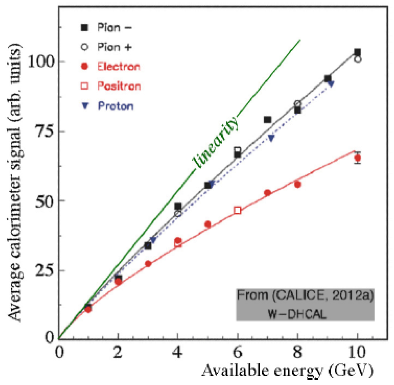
Figure 6.
Saturation effects in one of the towers of the SPACAL calorimeter (a). Shown are the average signal (b) and the energy resolution (c) as a function of energy, measured when a beam of electrons is sent into this tower.
Figure 6.
Saturation effects in one of the towers of the SPACAL calorimeter (a). Shown are the average signal (b) and the energy resolution (c) as a function of energy, measured when a beam of electrons is sent into this tower.

Figure 7.
The response to electrons and pions as a function of energy, for the CMS barrel calorimeter. The ratio of the total reconstructed energy in the CMS barrel calorimeter and the available beam energy for a variety of beam particles is shown as a function of energy. The different calorimeter sections were calibrated with electrons [19].
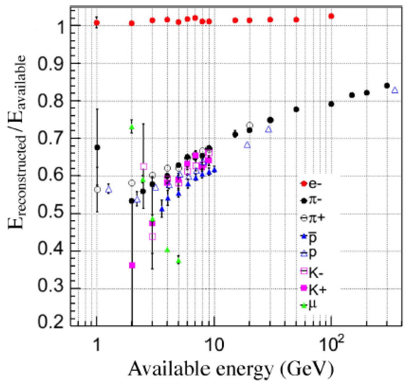
Figure 8.
Calibration procedures and resulting effects in the HELIOS calorimeter [20]. The calibration constants of the two longitudinal sections (a) of this calorimeter (A and B) were varied in order to minimize the total width of the electron signal distributions (b); The chosen value of the intercalibration constant leads to a signal non-linearity (c) for electrons. Even for the same energy (20 GeV), the average value of the signal depended on the number of s of which the showering electromagnetic object consists (d). See text for details.

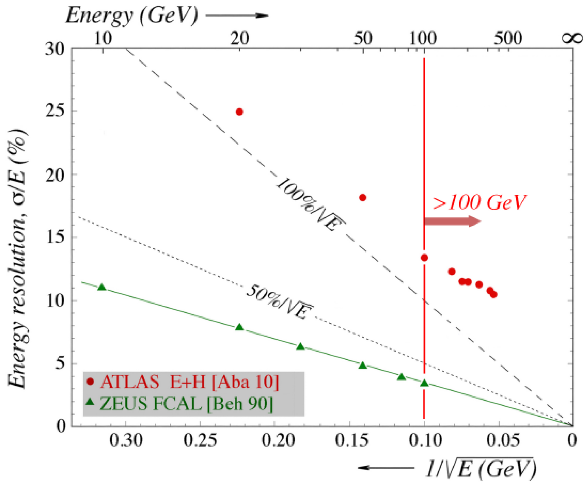
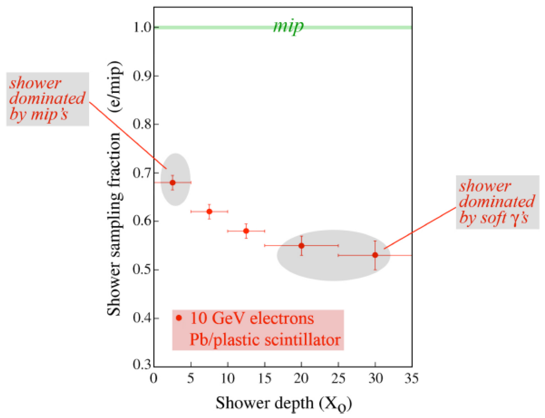
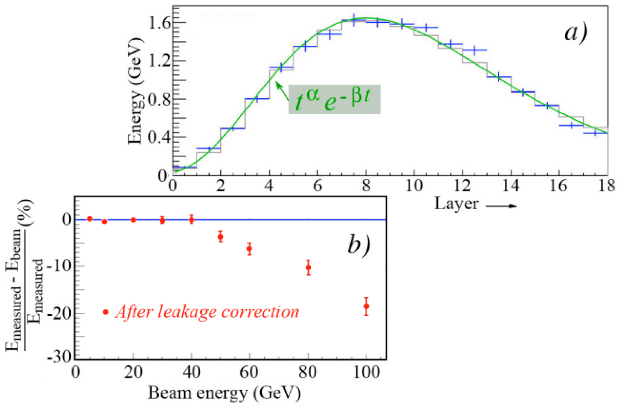
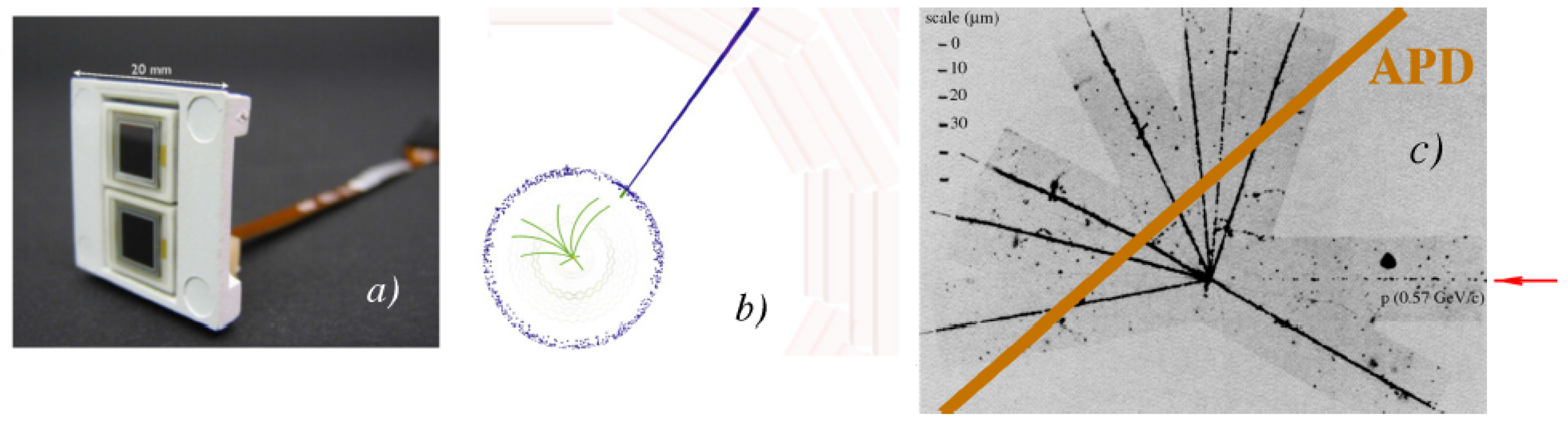
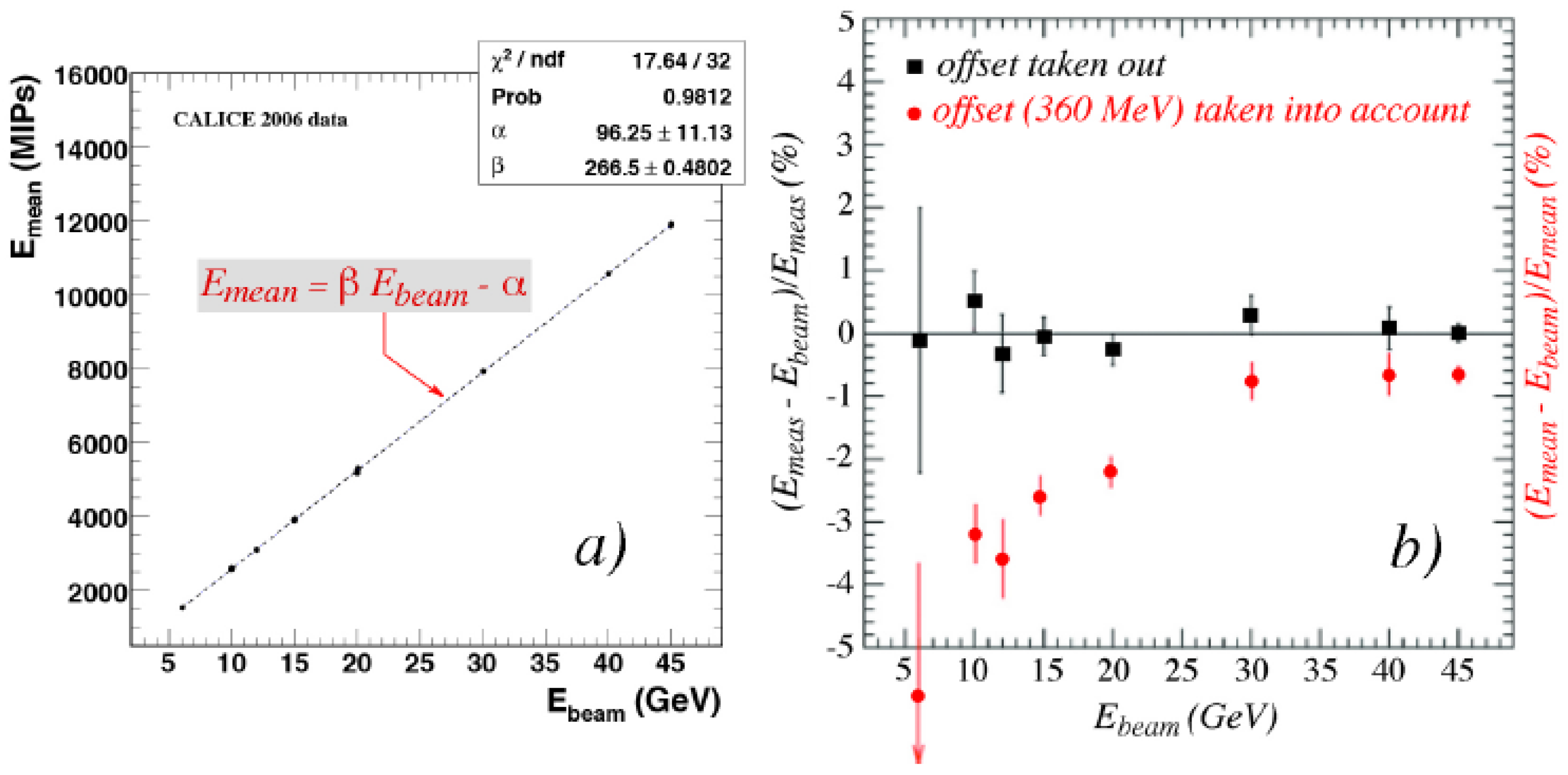
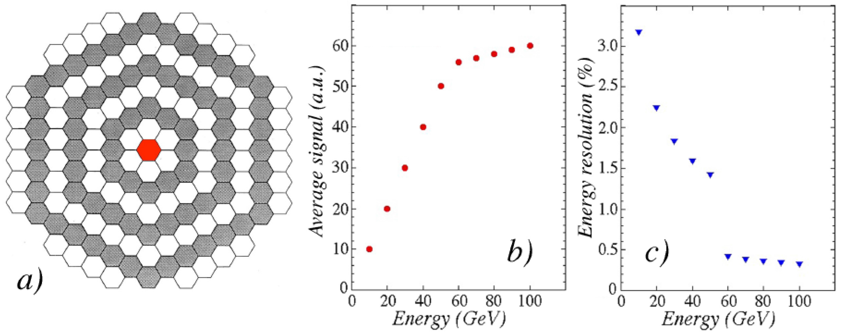
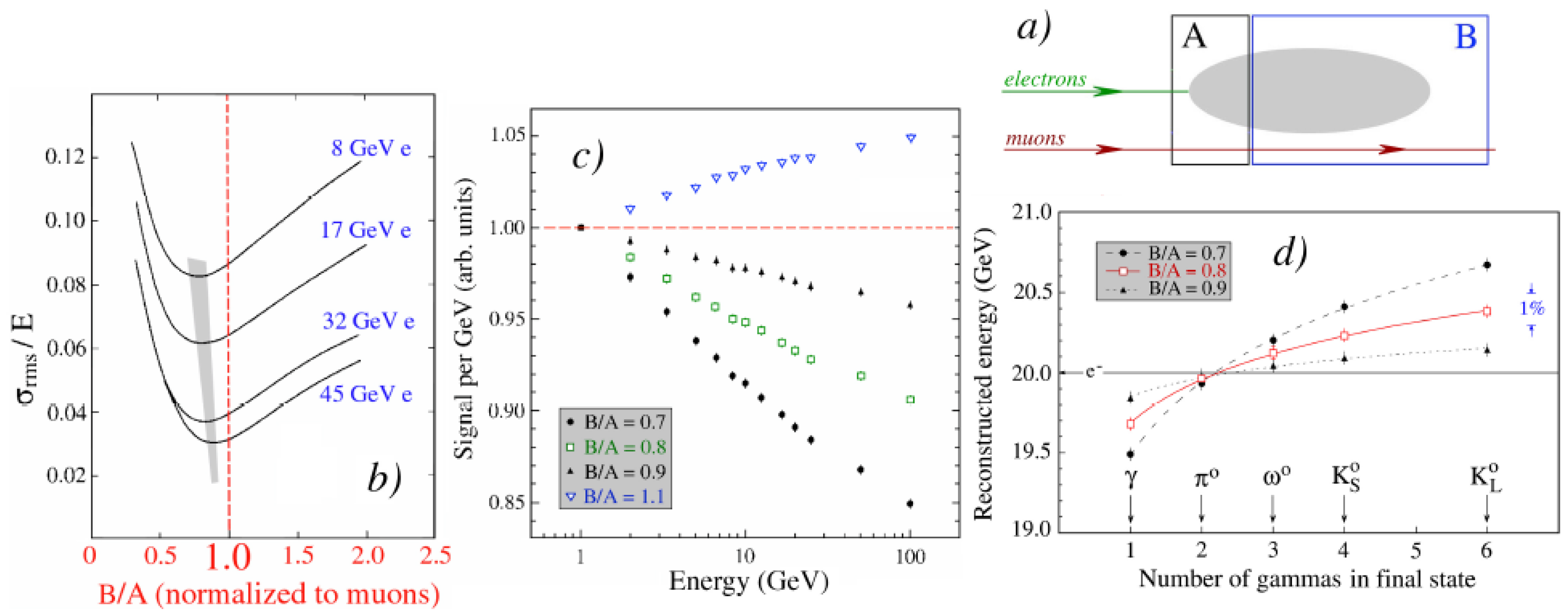
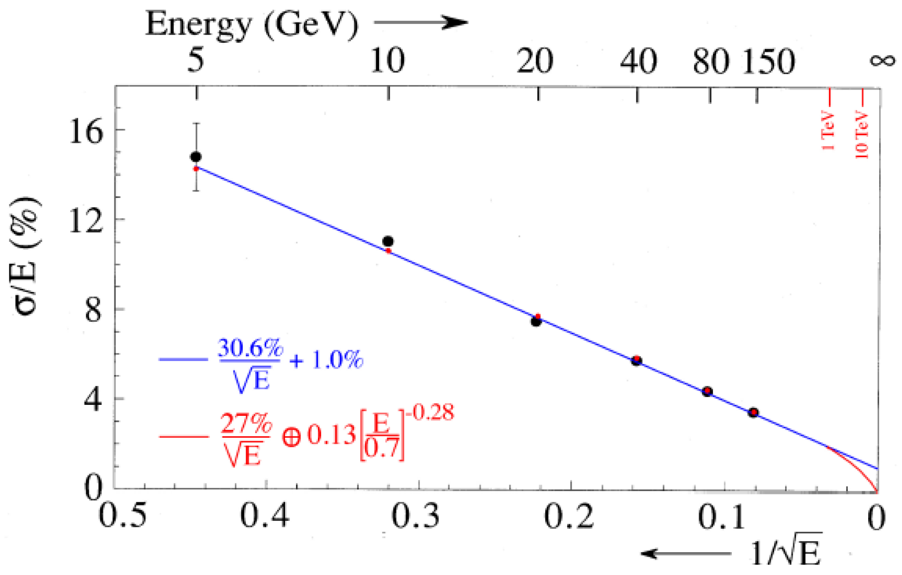
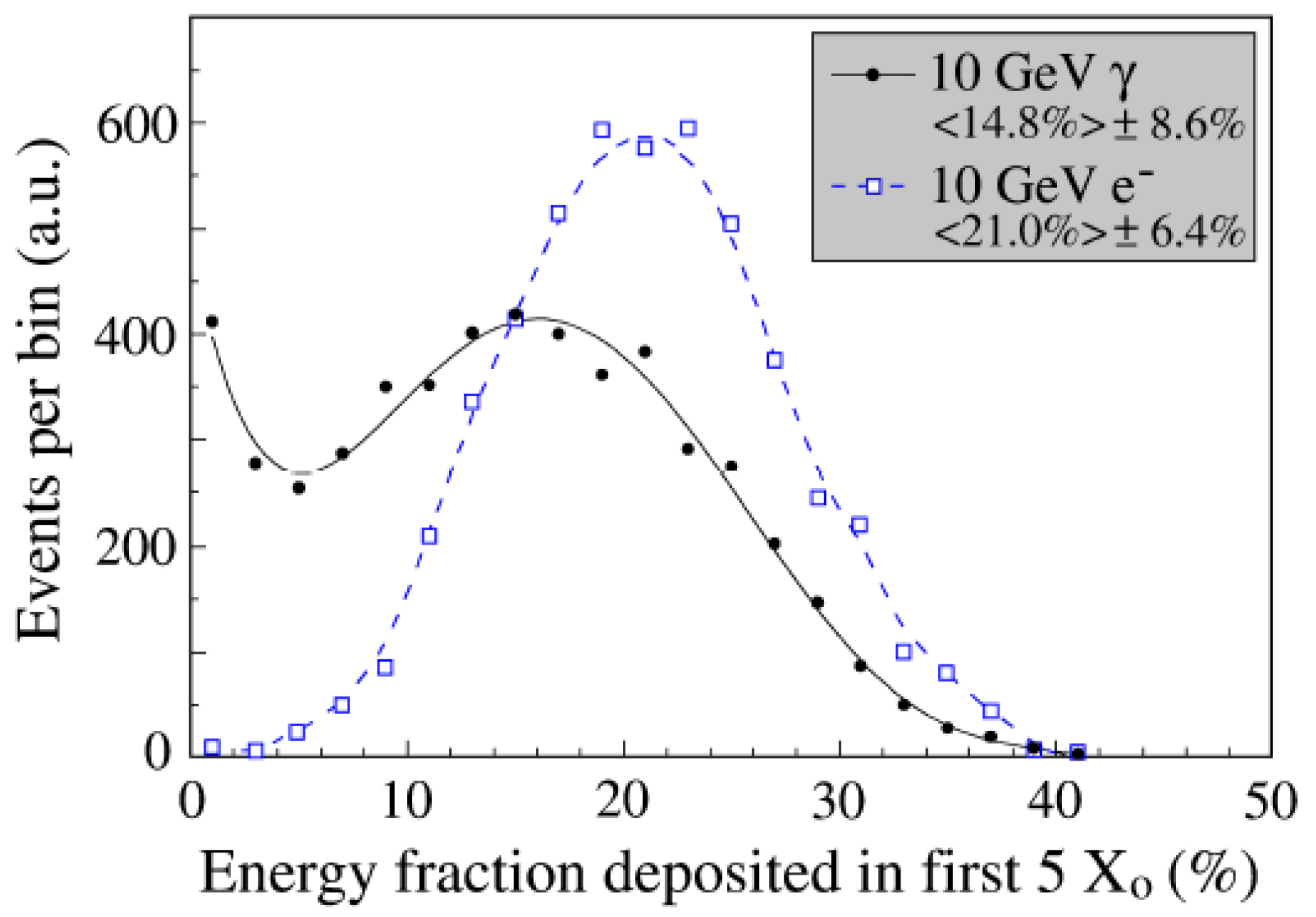
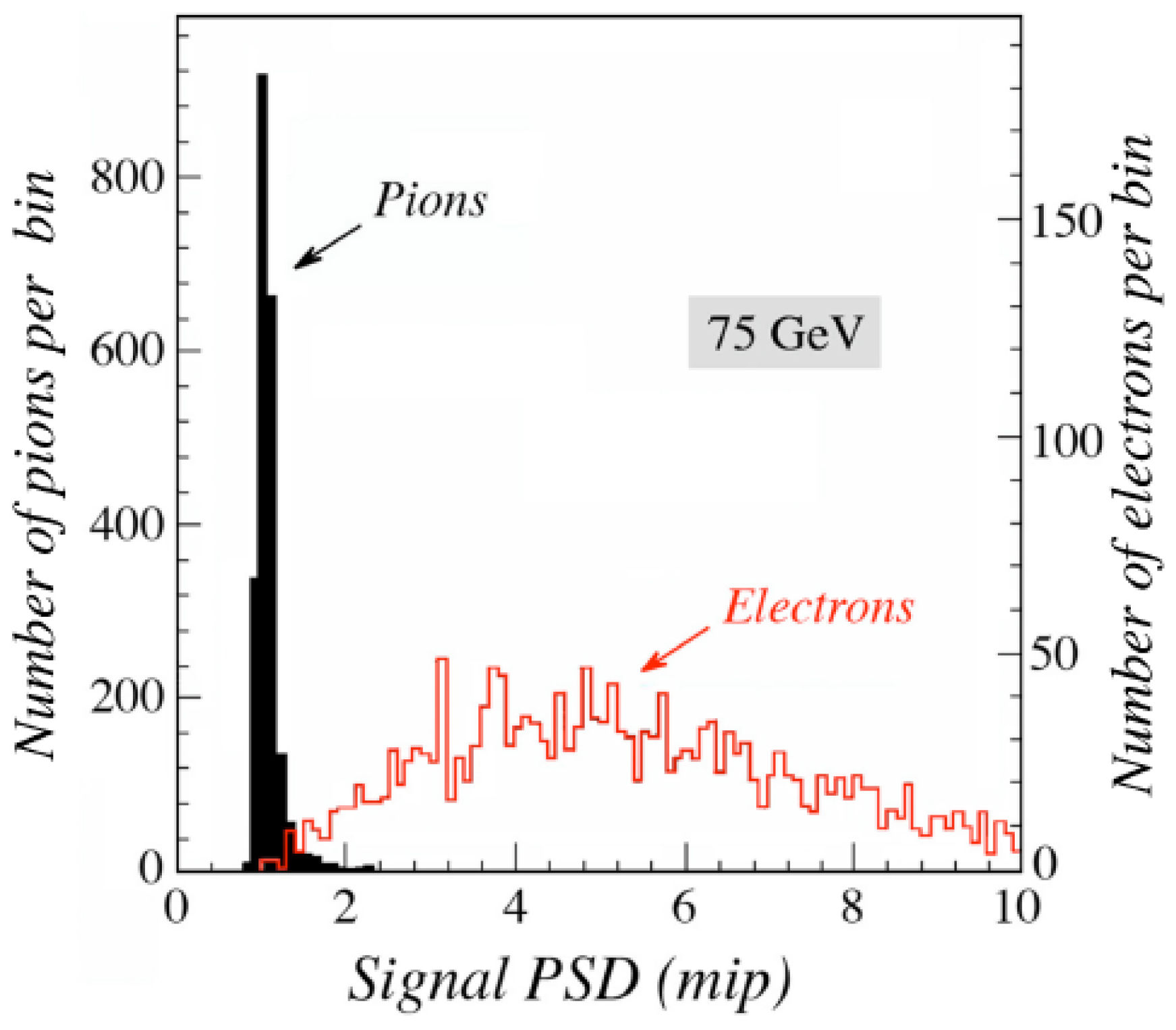
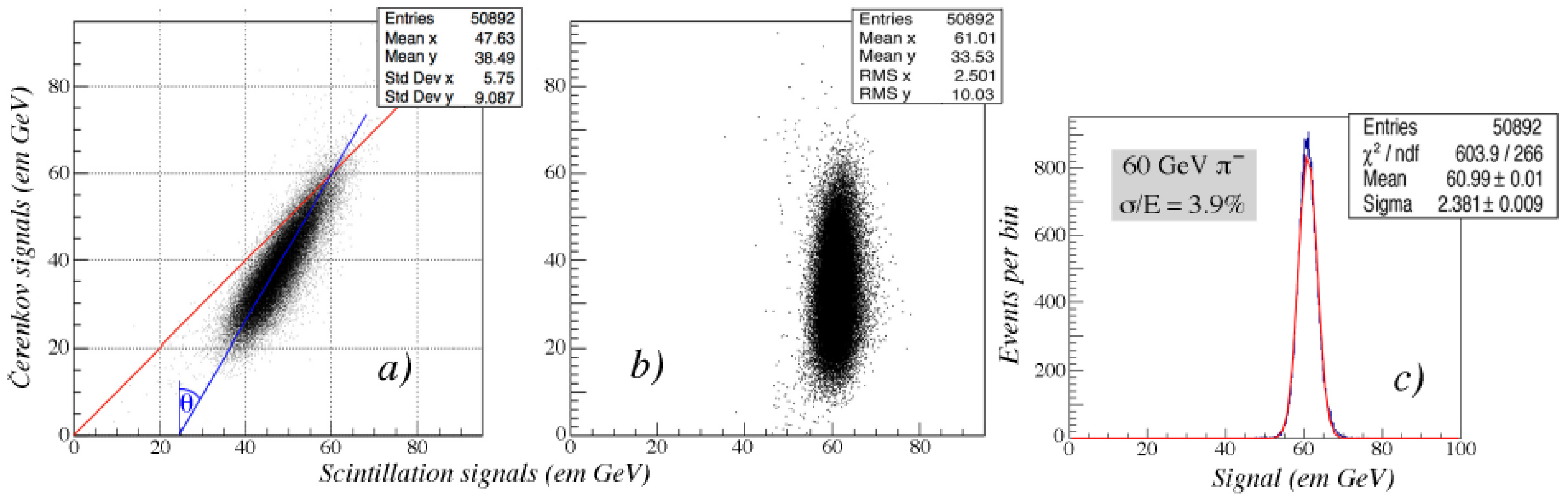
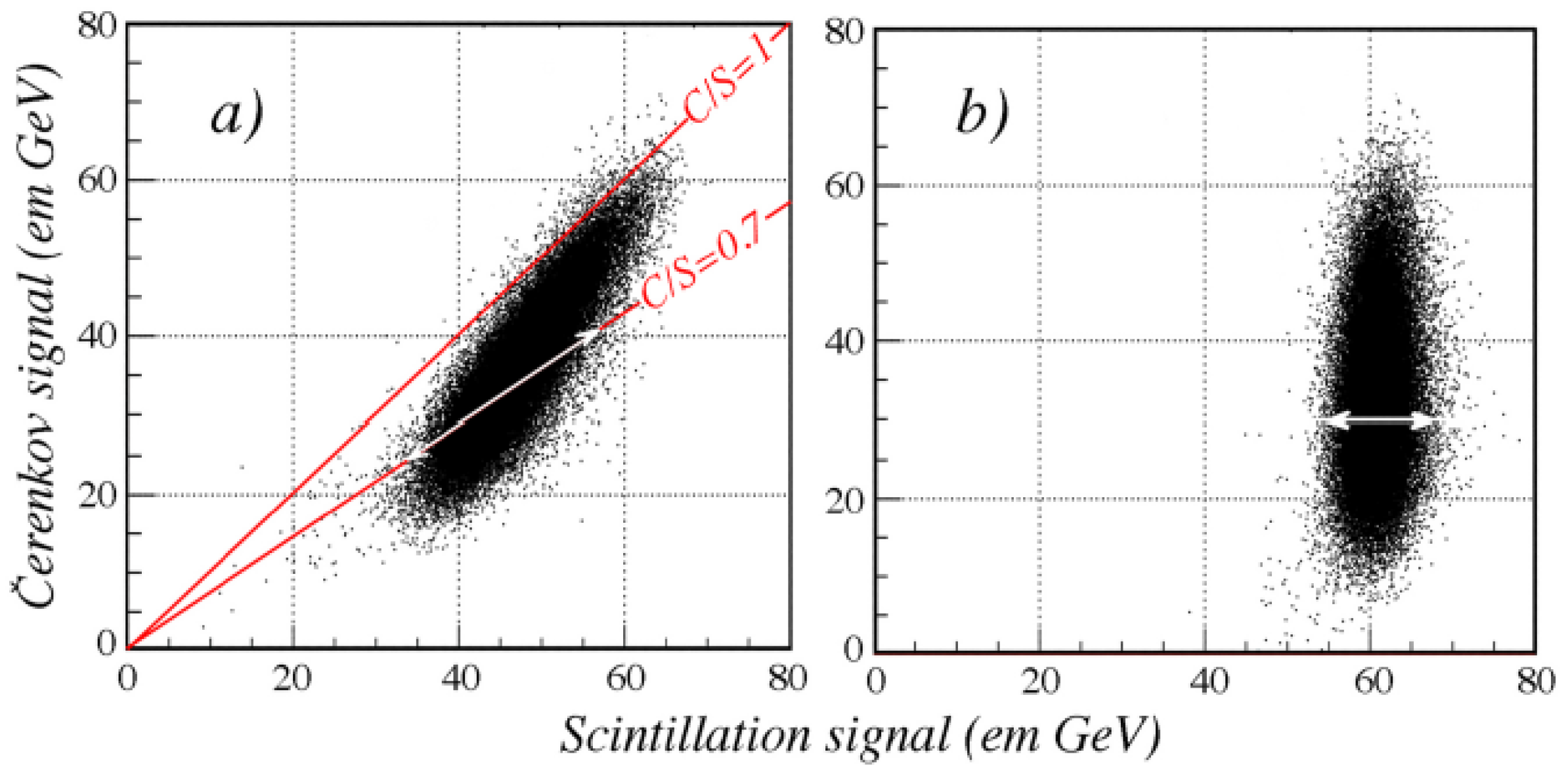
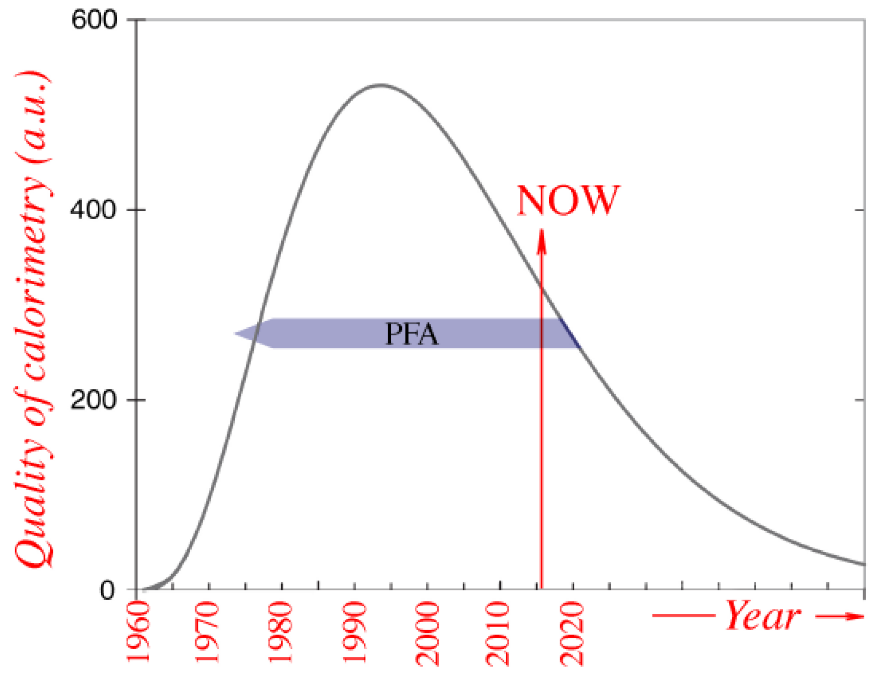
Figure 10.
Experimental data points for the hadronic energy resolution of the SPACAL lead/plastic-fiber calorimeter [4], together with two different fits of these data points. The differences between these two fits only become noticeable at very high energies, beyond the range where this instrument was tested.

Figure 11.
The distribution of the fraction of the energy of 150 GeV showers contained in the em shower core (a) [31] and the signal distribution for 300 GeV showers in a non-compensating calorimeter (b) [32].
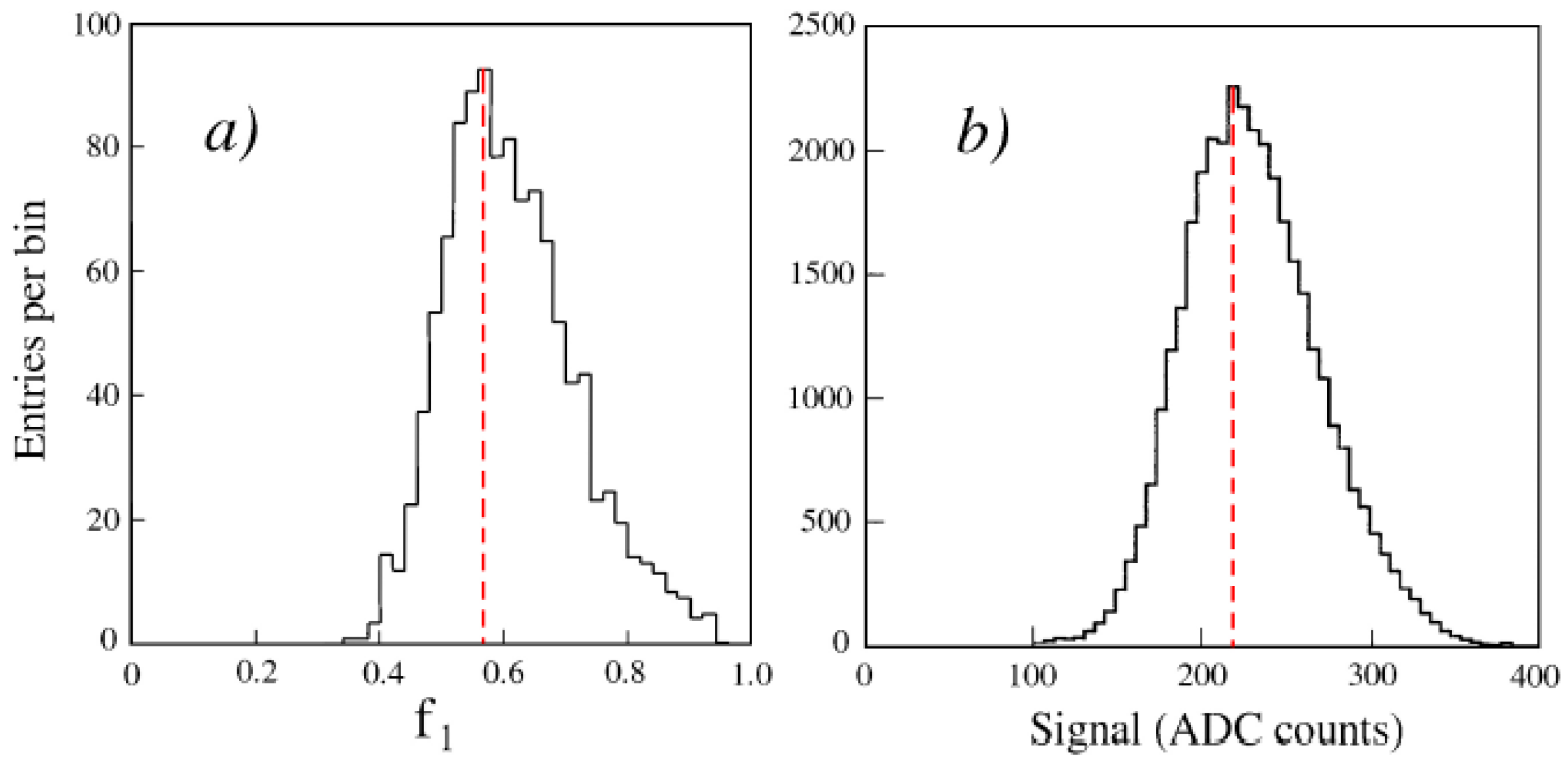
Figure 12.
Signal distributions for 300 GeV pions (a) and protons (b) in the CMS forward calorimeter. Average signals per GeV for protons and pions as well as the ratio of these response values in this detector, as a function of energy (c) [32].
Figure 12.
Signal distributions for 300 GeV pions (a) and protons (b) in the CMS forward calorimeter. Average signals per GeV for protons and pions as well as the ratio of these response values in this detector, as a function of energy (c) [32].
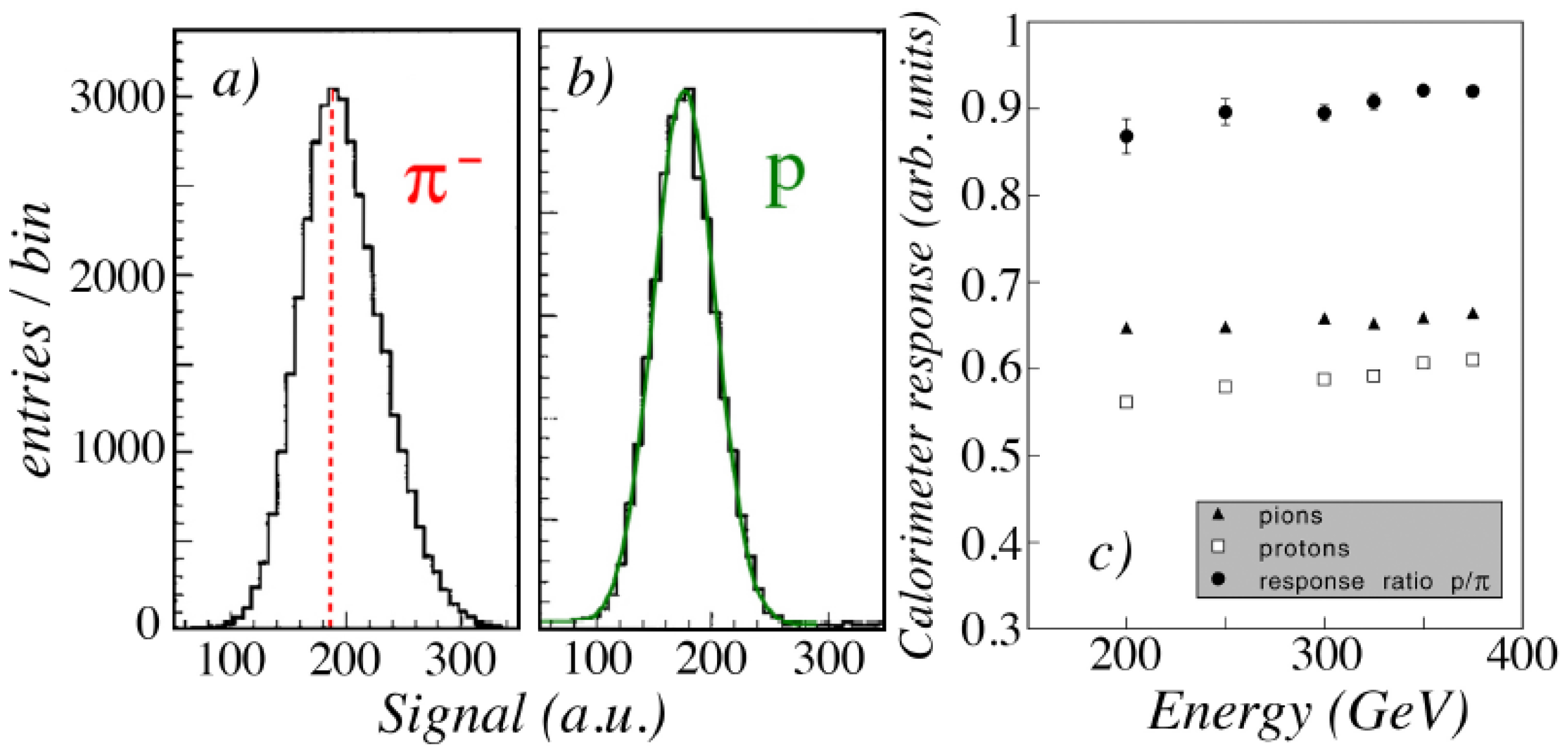
Figure 13.
Distribution of the energy fraction deposited in the first five radiation lengths by 10 GeV electrons and s showering in lead. Results of EGS4 simulations [21].
Figure 13.
Distribution of the energy fraction deposited in the first five radiation lengths by 10 GeV electrons and s showering in lead. Results of EGS4 simulations [21].

Figure 14.
The measured distribution of the starting time of the calorimeter’s scintillation signals produced by 60 GeV electrons (a) and 60 GeV pions (b); This time is measured with respect to the moment the beam particle traversed a trigger counter installed upstream of the calorimeter. These data were also used to determine the distribution of the average depth at which the light was produced in the hadron showers (c).
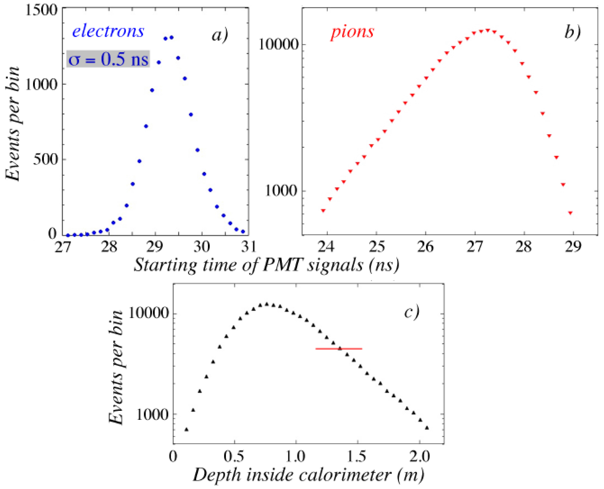
Figure 15.
Signal distributions for 75 GeV pions and electrons in a preshower detector used in beam tests of CDF calorimeters.
Figure 15.
Signal distributions for 75 GeV pions and electrons in a preshower detector used in beam tests of CDF calorimeters.

Figure 16.
Signal distributions of the RD52 Dual-Readout lead/fiber calorimeter for 60 GeV pions [36]. Scatter plot of the two types of signals as recorded for these particles (a) and rotated around the point where the two lines from diagram a intersect (b); Projection of the latter scatter plot on the x-axis (c).

Figure 17.
Scatter plots of the Čerenkov vs.the scintillation signals from showers induced by mono-energetic hadrons (a); The arrow indicates the precision with which the em shower fraction, and thus the energy, of an individual particle can be determined on the basis of the measured ratio of the Čerenkov and scintillation signals, 0.7 in this example. The rotation procedure for an ensemble of mono-energetic pions leads to the scatter plot shown in diagram (b). The precision of the measurement of the width of that distribution is indicated by a white arrow as well [36].

Figure 18.
The signal distribution for 60 GeV in the RD52 dual-readout lead/fiber calorimeter, for all events (a) and for events where the showers were contained in this detector (b). See text for details.
Figure 18.
The signal distribution for 60 GeV in the RD52 dual-readout lead/fiber calorimeter, for all events (a) and for events where the showers were contained in this detector (b). See text for details.
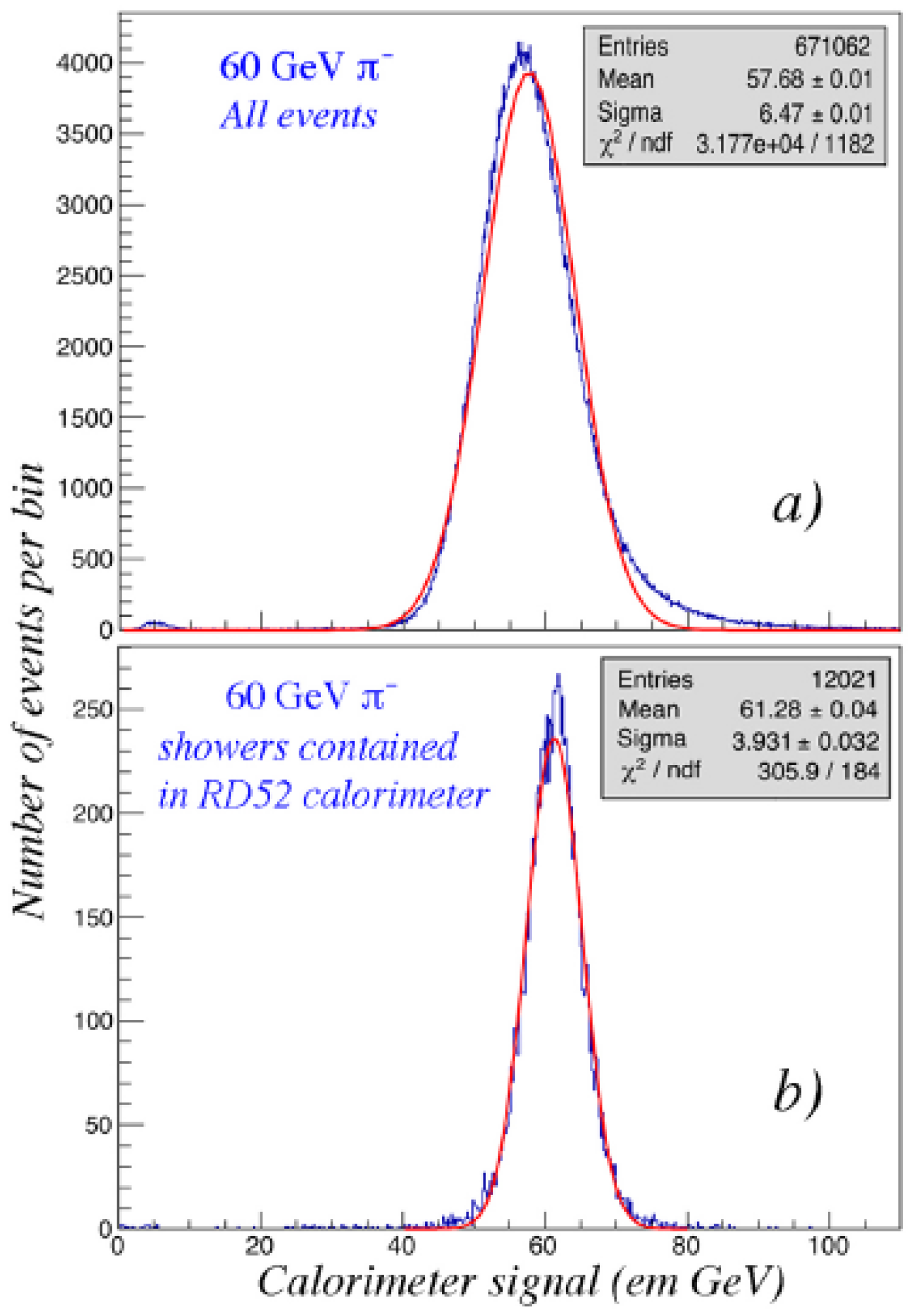
Figure 19.
The quality of calorimetry for particle physics experiments as a function of time. See text for details.
Figure 19.
The quality of calorimetry for particle physics experiments as a function of time. See text for details.

© 2017 by the authors. Licensee MDPI, Basel, Switzerland. This article is an open access article distributed under the terms and conditions of the Creative Commons Attribution (CC BY) license (http://creativecommons.org/licenses/by/4.0/).
Share and Cite
MDPI and ACS Style
Livan, M.; Wigmans, R. Misconceptions about Calorimetry. Instruments 2017, 1, 3. https://doi.org/10.3390/instruments1010003
AMA Style
Livan M, Wigmans R. Misconceptions about Calorimetry. Instruments. 2017; 1(1):3. https://doi.org/10.3390/instruments1010003
Chicago/Turabian StyleLivan, Michele, and Richard Wigmans. 2017. "Misconceptions about Calorimetry" Instruments 1, no. 1: 3. https://doi.org/10.3390/instruments1010003