Simplified Three-Microphone Acoustic Test Method


United States Department of Agriculture-Agricultural Research Services, Lubbock, TX 79403, USA
*
Author to whom correspondence should be addressed.
Instruments 2017, 1(1), 4; https://doi.org/10.3390/instruments1010004
Submission received: 22 February 2017
/
Revised: 22 June 2017
/
Accepted: 13 July 2017
/
Published: 28 July 2017
Abstract
:Accepted acoustic testing standards are available; however, they require specialized hardware and software that are typically out of reach economically to the occasional practitioner. What is needed is a simple and inexpensive screening method that can provide a quick comparison for rapid identification of the top candidates. This research reports on the development of an acoustical rapid-test method that achieves these objectives. The method is based upon a reformulation of the well-regarded three-microphone method. The new formulation reduces the number of required microphones to a single microphone and removes the need for simultaneous capture and extensive signal-processing analysis. The study compares the proposed simplified method to two standard methods and the three-microphone method. The results of the correlation analysis between the new method versus the original method produced a coefficient of determination of r2 = 0.994. A simulation study highlighted several unique accuracy advantages of this new proposed method in comparison to the existing standard methods. The proposed new method represents an easy-to-use technique that requires little in the way of equipment and can be set up with minimal training and expense.
1. Introduction
In acoustic testing, well-accepted standards are available for testing samples in reflection of samples backed by a hard reflector. These methods were first developed utilizing microphones inside a closed tube with the sample held against a rigid plate, with the other side providing the sound generation source. Seybert [1] pioneered the use of utilizing microphone measurements at two spots in the tube spaced away from the sample to calculate the reflection coefficient due to the sample’s interaction with the incoming sound pressure wave. By utilizing a broad-band white-noise source, the method dramatically reduced the testing time of one of the first standard methods, in comparison to the original single-frequency excitation first-principle method that directly measured the standing-wave ratios inside the tube, ISO-10534-1 [2]. Later Chung and Blaser [3,4] furthered the art by providing a calibration technique that allowed for the use of two microphones taking simultaneous measurements. The combination of these methods allowed for rapid testing of samples backed by a hard-reflector. This new methodology was later standardized into the now well-known “two-microphone” test-methods, ASTM E1050 and ISO-10534-2 [5,6]. It is of note that while these test methods are valid and a good predictor for acoustic absorbers when utilized in reflection-type applications that are backed by solid objects, such as brick walls, they do not provide an accurate means to predict how a sample will react when placed into a sound-shielding-type application, such as preventing sound from moving from one room to another. To clarify why the reflectance measurement cannot be used is found with a mirror analogy. In the standard’s reflectance tests [2,5,6], the measurement utilizes a near-perfect reflection plate to back the sample. Thus, the measurement is reliant upon the test sample to absorb the acoustic energy. Thus, any energy reflected off the front surface of the material is not readily separable from the energy reflected by the backing plate, as the only difference between the two is a phase shift between the two waves. Hence, this method is only able to measure the energy absorbed by the material. To see the error in this method, we note that a mirror would provide a near-perfect reflection, yet absorbs almost nothing. Thus, a test utilizing the strength of the reflected light would incorrectly report it as a poor acoustical absorber. However, if this same mirror was used for room-to-room acoustic shielding, it would perfectly reflect all the incoming sound, leaving the occupants in the next room to sit in perfect silence, even despite that the mirror did not absorb any sound energy. Thus, in essence, the mirror is the perfect sound shield, yet the standard reflectance test methods [2,5,6] would report it as a poor performer. From this analogy, it is clear that a different method is required for through-transmission applications, especially for materials that act more like mirrors than sound absorbers. Typically, this is the case as materials increase in density, as high-density materials make excellent sound reflectors. Thus, for through-transmission sound shielding, these materials work wonderfully, yet the standard reflectance test methods [2,5,6] cannot be utilized for this type of testing. What is required is a true through-transmission measurement that can measure the material’s propagation coefficients.
Acoustic testing for through-transmission applications is still an active area of research [7,8,9]. To date, only the ASTM E2611 [10] has accepted a proposed method for this, the four-microphone method, while the ISO body has not ratified this method due to concerns about accuracy. In summary, each of the methods proposed in the literature work well for certain test conditions and types of samples, but none work universally well. A recent review of the most promising methods was performed by Salissou and Panneton [8], who reported on testing several of the most promising through-transmission techniques and the accuracy and usability of each method. In their study, they performed testing of three candidates that were comprised of low-density fibrous-type materials. They were: 51 mm thick melamin foam (density of 9 kg·m−3), 42.5 mm thick glass wool (density of 40 kg·m−3), and 76 mm acoustical/thermal insulator wood (density of 38.5 kg·m−3). The techniques they reported on were:
- The two-microphone dual cavity-backed method [13].
- A modified variant of the Iwase method [14] that utilized microphones on both sides of a sample backed by a hard reflector, with no air space between the sample and the reflector. The modification was to utilize a two-microphone method up-stream, versus the original Iwase method that used a microphone directly on the surface of the sample. They noted that their proposed modification enhanced the speed and utility of the original Iwase method. Of note however, is that this modification was only designed to streamline the test method for speed. It was not designed to improve the accuracy of the method.
Doutres, Salissou and Panneton recently reported [7] on a comparison of several techniques, noting that the most accurate of the tested methods was the modified Iwase [14] method, which outperformed two different variants of the four-microphone method, where the improvement was most notable in the low frequencies—which we note is where the attenuation coefficient is the smallest. Given their reported results, the authors of this study examined and utilized both the original and the modified Iwase method for the through-transmission study. During test evaluations utilizing this method, the authors developed a simplified reformulation of the original Iwase equations that allowed for use of a simplified experimental apparatus utilizing only a single microphone to obtain the main metrics for sound shielding: the acoustic absorption coefficient, the reflection coefficient and the acoustic propagation attenuation constant, which are directly applicable for computing the propagation loss as the acoustic wave propagates through the material.
This report is organized by first developing the new proposed variant of the Iwase [14] formulation, thereby proving mathematical equivalence. This theoretical basis is then followed by a simulation study comparing the performance of the various methods when subjected to injected noise. Finally, the research will provide experimental results illustrating practical equivalence of the new methodology. The experimental phase was performed utilizing a comparison test contrasting the results for a wide range of materials with a wide span of densities, to achieve a wide range of reflectance values and material attenuation properties. Finally, critical application details for using the new proposed methodology are provided.
2. Materials and Methods
2.1. Theoretical Derivation
The acoustic testing apparatus for this research utilizes the impedance tube, otherwise known as Kundt's tube. The tube is a resonant structure whereby sound is inserted into one end and is reflected at the other end, yielding standing waves inside the tube that are then analyzed to extract the acoustic properties of the material under evaluation. This type of acoustic testing has a rich history for evaluating open-cell porous media for the prediction of performance properties of various materials used in noise-abatement applications [1,3,4,7,12,13].
Sound radiation inside an impedance tube can be modeled as an incident plane wave “Pi” traveling in one direction that is combined with a second reflected wave “Pr” traveling in the opposite direction [the “P” denotes the pressure of the wave] [9,12]. This simple model performs admirably in the prediction of the standing wave phenomena that occurs inside the impedance tube. Augmentation of the model allows for predicting the influence of an inserted material on the propagating waves. In the time domain, the two waves are typically modeled utilizing the following complex-valued equations (where complex vectors are constructed from phase and magnitude values of the pressure waves, known also as phasors):
where Pi(x,t) is the incident wave as a function of x and t, Pr(x,t) is the reflected wave as a function of x and t, |Pi| is the magnitude of the incident wave, |Pr| is the magnitude of the reflected wave, t is time (s), j is complex value where j = sqrt(−1), and x is position with respect to the sample surface (m). The propagation wave number of the acoustic wave in air (rad·m−1) is given by ko, and ω is the frequency of the sound wave (rad·s−1).
Pi(x,t) = |Pi| e(−jk°x + θi) e(jωt)
Pr(x,t) = |Pr|e(jk°x + θr) e(jωt)
Equations (1) and (2) are then translated to the frequency domain and combined into Equation (3):
where P(x) is the pressure at location x, k is the propagation wave number of the acoustic wave inside the material (rad·m−1).
P(x) = Pi(x) + Pr(x) = |Pi| e(−jkox) + |Pr| e(jkox)
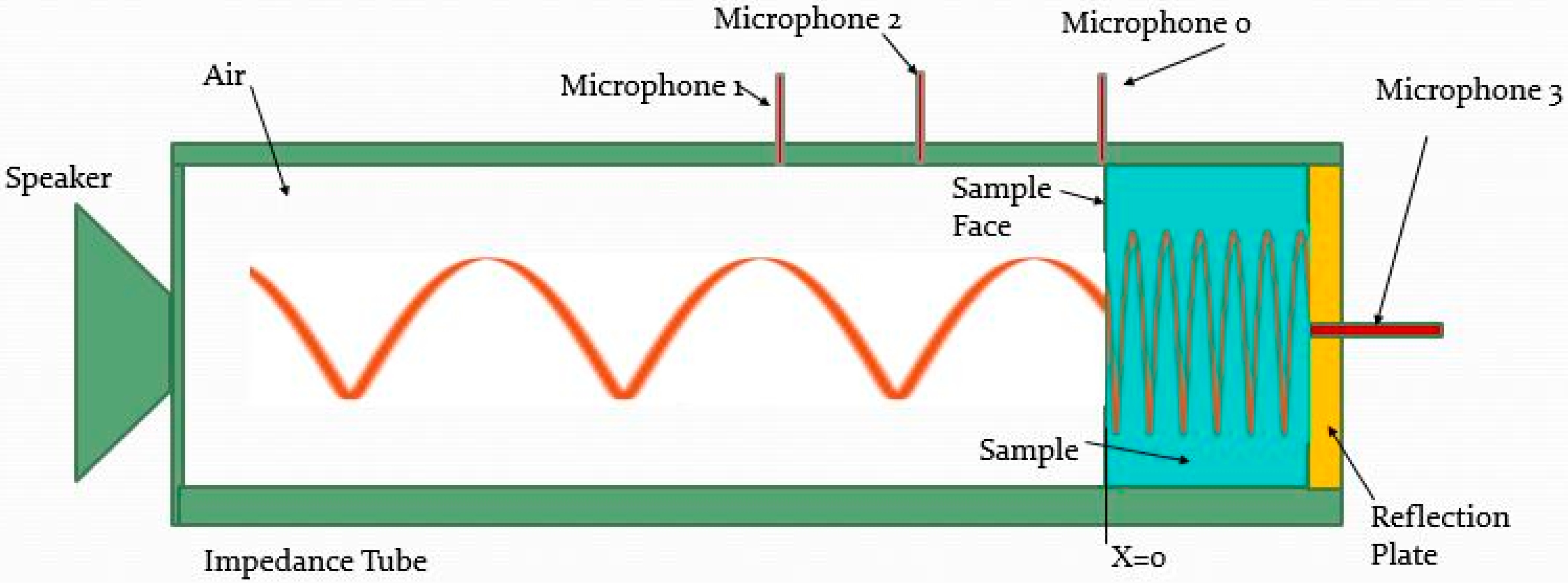
For use in the development of the model, Figure 1 shows the schematic outline, which also indicates key microphone locations along with the x-position definition.
Utilizing this map, Iwase et al. [14] provided the following derivation to develop the three-microphone method (using microphones 0, 2 and 3 positions as detailed in Figure 1). As the derivation of interest for this article will be taking this model in a different direction, we will reproduce the initial derivation here so that it becomes clear where we deviate and branch off to the new proposed alternative technique, hereafter known as the “simplified Iwase method” (SIM). Of note is that the modern variant of the three-microphone method omits microphone 3 and practices the two-microphone method to obtain the reflection coefficient utilizing microphones 1 and 2. Thus, in essence, this derivation also extends the standard two-microphone methods [5,6], whereby microphone positions 1 and 2 are located as in the standard methods. As such, it begins utilizing the same approach that was used in the two- and three-microphone methods’ development. Equation (4) details the pressure wave as measured by a microphone located at position 1, where the measured pressure is due to both the incident and reflected waves (Pi and Pr, respectively):
P1 = Pi e(jko|x1|) + Pr e(−jko|x1|)
Equation (5) details response for the microphone at position 2:
P2 = Pi e(jko|x2|) + Pr e(−j ko|x2|)
Iwase, in his report, added an additional microphone, at the face of the sample, labeled microphone 0 (Figure 1). The response for microphone 0, at x = 0, provides Equation (6):
where PM0 is the pressure at the location corresponding to microphone 0.
Pf = PM0 = Pi + Pr
From wave theory, a plane wave in a source-less region propagating along a one-dimensional path can be used to model the effect of the material on this wave by utilizing the complex propagation coefficient for the material: γ = α + jβ [6,12], where α is the material propagation attenuation constant and β is the material propagation phase-delay constant. Including the propagation constant for the material allows for characterizing Pr in terms of Pi, as modified by transport through the material twice (forward and back). Of importance to note here is that for many materials, reports have been provided for which α is not constant across the frequency spectrum and is, for some materials, a function of the frequency [15,16,17]. Prime examples of materials that exhibit this behavior are water, metals and other crystalline objects [18]. The literature reports, noted above, report success in utilizing a simple power-law model that describes how α changes with frequency, and is shown here for convenience in Equation (7):
where η is the exponential correction term, αo is a very low frequency value for the propagation attenuation constant α, and f is the frequency (Hz).
α = αo (2πf)η
The advantage of utilizing the propagation constant of the material is that it allows for modeling how the wave is modified as it propagates through the material under test, which can then be used to provide an estimate of absorption characteristics as the sample size changes. In the analysis, α is brought in via a transition from Equations (6) and (7) to provide Equation (8):
where R is the reflection coefficient (dimensionless).
Pr = Pi e(−2dγ) = Pi R
R = e(−2dγ) = e(−2d[α + jβ])
= e(−2dα) e(−2 jβd)
= e(−2dα) e(−2 jβd)
|R| = e(−2dα)
Combining Pi and Pr yields the pressure Pf at the sample surface (location of microphone 0), which is shown in Equation (9); noting Pr = Pi e(−2γd) provides
Pf = PM0 = Pi + Pr
Pf = Pi + Pi e(−2γd)
Pf = Pi + Pi e(−2γd)
Also of interest to the derivation is the pressure that occurs after the sound propagates through the material to arrive at the rear of the sample, at the location of microphone 3, which is written as Equation (10):
Pbi = Pi e(−γd)
The rear of the sample is backed by a near-perfect reflector; thus, in addition to the incoming wave Pbi, there is also the reflected pressure wave, Pbr, at the microphone 3 location and shown as Equation (11):
Pbr = Pi e(−γd)
As the incident and reflecting pressure waves are co-located at location 3, the microphone measures
PM3 = Pbi + Pbr = 2 Pi e(−γd)
The next step utilizes the ratio of measurements taken at the microphone face (location 0), with respect to the microphone on the backside of the sample, at the hard reflector (location 3). This yields the transfer function between locations 0 and 3. At this point we deviate slightly from the Iwase approach and simplify the ratio utilizing hyperbolic trigonometric identities:
H30 = PM0/PM3 = [Pi + Pi e(−2γd)]/(2 Pi e(−γd))
= ½ (e(γd) + e(−γd))
= ½ (e(γd) + e(−γd))
Then, utilizing a hyperbolic identity leads to
H30 = cosh(γd)
This can then be inverted to provide the acoustic propagation constant as shown in Equation (13), which provides the basis for our proposed two-microphone variant of the three-microphone method, hereafter termed the CSMM method, Complex-Single-Microphone-Method, which could also be performed with two microphones at locations 0 and 3; as opposed to the ASTM E1050 two-microphone method that utilizes two microphones at locations 1 and 2.
γ = acosh(H30)/d
For the computation of the reflection coefficient, we note that it is not necessary to utilize two internal microphones, as per the applied method in the normal application of the three-microphone method (Salisslou). In lieu of this, we note that R can be computed directly from the propagation coefficient γ per Equation (14), which is a re-statement of Equation (8):
R = e(−2γd)
Of importance to note here is that Equation (13) requires the use of the complex quantity H30; as such, the measurement must measure the phase as well as the magnitude.
For a simpler experimental variant of the CSMM method, we examine the potential for the removal of the phase measurement from H30. Starting with the definition of H30,
H30 = PM0/PM3 =[Pi + Pi e(−2γd)]/(2 Pi e(−γd))
= ½ (e(γd) + e(−γd))
= ½ [e(d[α + jβ]) + e(−d[α + jβ])]
= ½ (e(γd) + e(−γd))
= ½ [e(d[α + jβ]) + e(−d[α + jβ])]
We then break out the attenuation from the phase, yielding
H30 = ½ [e(dα) e( jβd) + e(−dα) e(−jβd)]
In the time-domain, this becomes
which unfortunately is not readily transformed to a simpler form that can utilize only the magnitude. It is instructive to note, however, that the results suggest that errors will result if phase information is ignored. Hence, this derivation will now pivot to an alternative approach.
H30 = ½ [e(dα) cos(ωt + βd) + e(−dα) cos(ωt − βd)]
H30 = ½ [e(dα) {cos(ωt)cos(βd) − sin(ωt)sin(βd)} + e(−dα) cos(ωt − βd)]
H30 = ½ [e(dα) {cos(ωt)cos(βd) − sin(ωt)sin(βd)} + e(−dα) cos(ωt − βd)]
From this point we extend beyond the Iwase solution to create an equivalent single-microphone method (SSMM, Simplified-Single-Microphone-Method) that provides the benefits of a near-equivalent measurement with the benefits of providing a lower cost and easier method to put into practice, with much flexibility in the final form of the apparatus.
In moving forward to the new proposed SSMM, we propose a formulation basis for a method that only requires a single microphone or sound meter installed into the end of the tube. Use of a sound-level meter is particularly advantageous, as then no other instrumentation will be required, and results can be easily calculated from a few readings on the sound-level meter. The drawback to the sound-level meter is that as it is integrating over the spectrum, two samples could provide the same reading, yet yield very different responses across the spectrum. Hence, we recommend this approach is only used for screening purposes, and for all others, it is better to collect the data with a microphone and oscilloscope or audio data-acquisition system. The different versions of this new SMM, {SSMM or CSMM} protocol will be discussed in detail in a later section. For this section, the theory showing the equivalence for using a single microphone to obtain equivalent readings will be detailed next.
The basis for the proposed new SMM formulation is to take two measurements at the microphone 3 location (at the back of the material against the hard reflection plate; Figure 1). The first measurement is performed with the material inserted into the sample holder, and the second measurement, an air reference, is performed without the material under test. The following derivation follows the two-microphone and Iwase theoretical derivations. The derivation for this approach looks to establish a simpler formation of a transfer function between the air reference reading, that is then taken with respect to the measurement with the material in place, yielding a new transfer function H33 as shown in Equation (15), using Equation (12) as the expression for PM3:
H33 = PM3/PM3air = [2 Pi e(−γd)]/[2 Pi e(−γaird)]
= e[−d (α + jβ)]/e[−d (αair + jβair)]
= e[−d (α + jβ)]/e[−d (αair + jβair)]
Given that over the short distance of d, αair = 0, then converting into the time domain leads to Equation (16):
H33 = [e(−αd) cos(ωt − βd)]/[cos(ωt − βaird)]
Then, a simplification of Equation 16 leads to Equation (17):
where θ = d(β − βair) is the relative phase between the sampled signal to the air reference reading.
H33 = e(−αd) cos(ωt − θ)
= e(−αd) cos(ωt − d(β−βair))
= e(−αd) cos(ωt − d(β−βair))
Of importance from this relation is that in the time domain, the cosine term of Equation (16) is only relevant to the phase of the signal, as the peak-to-peak signal is solely controlled by the attenuation term e(−αd). Hence the attenuation of the signal, as induced by the presence of the sample, is readily obtained by measuring the time-averaged signal strength with and again without a sample in the test cell, and then taking the ratio of the two measurements. In practice, the measurement of the sound pressure level utilizes a measurement of the root-mean-squared (rms) value of the signal, which in the discrete form of a time-averaged version of the magnitude of H33 is provided by Equation (18):
where |H33|RMS is the rms estimate of the magnitude of H33, and n is the number of readings to perform the sum of squares over.
|H33|RMS = [(1/n) (∑ (H33)2)]0.5
Noting further that the rms value of a sinusoid is equal to the amplitude of the signal divided by the square-root of two allows for further reduction, which leads to the result from the time-averaged reading of Equation (18) to be simplified to the form of Equation (19). This application can be performed by replacing the sinusoidal oscillator with a measurement of the peak-to-peak or rms voltage, as shown in Equations (17) and (18), for the sample and air reference readings, which in the ratio, drops the input signal out to yield the magnitude ratio |H33|RMS that provides Equation (19).
|H33|RMS = e(−αd)
|PM3|RMS = Vpp_signal e(−αd)/(2)0.5
|PM3 air|RMS = Vpp_signal/(2)0.5
From Equation (19), a simple inversion provides the acoustic material propagation attenuation constant α of Equation (20) that is the final form of the SSMM method.
α = ln(|H33|)/d
For the determination of the normal incident acoustic absorption coefficient ρ, this can be computed using the reflection coefficient, by using α as determined from Equation (20) to compute |R|, as detailed in Equation (8), to provide ρ, as shown in Equation (21).
where |R| = e(−2dα) (Equations (8) and (14) re-stated for clarity), and ρ is the acoustic attenuation constant (dimensionless; range of 0–1).
ρ = 1 − |R|2
In summary, the equivalence derivation shown above provides the basis for two variants to obtain the acoustic reflection coefficient and the material’s propagation absorption coefficient. The first method, CSMM, provides a mathematically equivalent (identity) method to that obtained by the two-microphone method of ASTM E1050. Of particular interest is that the CSMM method not only provides R, but also provides a true measurement of the through-transmission propagation coefficient γ = α + j β, which is not available from the two-microphone approach. CSMM does this by capturing the single-microphone relative amplitude and relative-phase information. As such, it provides the primary information that is currently only obtainable utilizing the three- or four-microphone methods; which results in considerable savings in equipment and complexity, as it only requires two microphones, pre-amplifiers and data-acquisition channels. The next variant this analysis provides is the SSMM method, which is a low-cost means for the determination of the primary material acoustic of the propagation attenuation coefficient α. Where the SSMM method only captures the single-microphone relative amplitude information. In addition, this can be achieved from a greatly simplified acoustic test apparatus that can be as simple as a single microphone or a sound meter mounted onto the end of the tube. As with any new proposed method, of primary interest is the expected accuracy.
2.2. Accuracy
In light of the fact that there are several different methods for obtaining the same results, of interest are the trade-offs in cost and accuracy between the various methods. As was shown in the previous section, for the computation of the reflection coefficient R, the full SMM method utilizing the complex measure of H30 is a mathematical identity to the other standard methods; as such, theoretically they should all provide exactly the same value. Hence, of primary interest is how the standard methods compare to:
- The simplified variant of the SMM method, SSMM (|H33|; pressure magnitudes only).
- The complex SMM variant the CSMM (H30; pressure and phase).
- The simplified variant of CSMM (|H30|; pressure magnitudes only).
Of note is that method 3, CSMM (|H30|), was not derived from first principles; as such, the simulation study did not include noise, but instead examined how large the error was when the full complex values with phase information were not captured in the measurements. Of potential interest for this variant is in the application for online systems, where it is inconvenient or impossible to obtain an air-reference, periodically throughout the day, that would preclude the use of the SSMM (|H33|) method, while still preserving the ease and simplicity of a magnitude-only version.
All of these issues will be explored utilizing the Monte-Carlo simulation that studied the performance of the afore-mentioned methods with respect to the standard methods [2,5,6]. As the three-microphone method, in practice, [7,8,9,14] utilizes the two-microphone method for the computation of R, only the two-microphone comparison is reported on herein, as this also implicitly includes how well the three-microphone method would perform in the prediction of the reflection coefficient R. Thus, the performance comparisons will be made for the following techniques, in the presence of noise: SWR, Standing-Wave-Ratio [2], and the two-microphone method [5,6].
2.2.1. Accuracy Comparison in the Presence of Noise
As both of the SMM methods provide mathematical identities to the two-microphone method, for the prediction of the reflection coefficient R, of primary interest is how the CSMM and SSMM methods compare to the standard SWR [2] and two-microphone methods (ASTM E1050 and ISO 10534-2) [5,6] when the measurements are subjected to experimental noise. Of note is that the three-microphone method utilizes the two-microphone method in the measurement of R. To explore each of the methods’ ability to extract the correct estimate of R in the presence of noise, an accuracy comparison was performed, utilizing a simulation study to examine the performance of the prediction equations in an idealized theoretical solution that allowed for a full exploration across all the variables of interest, with the two main variables of interest being the attenuation and phase-delay terms in the material propagation constants. As the prediction of R implicitly utilizes a measure of the material propagation constant α, this study effectively tested this performance metric as well. The analysis was performed utilizing a Monte-Carlo simulation to predict the pressures inside the impedance tube for any given sample thickness and material properties, with and without added Gaussian white noise, at a relative signal-to-noise level of 0.005, for a typical sample thickness of 19.05 mm at a temperature of 23 °C. The locations of microphones 1 and 2 were placed at 0.07 and 0.03 m, respectively.
2.2.2. Accuracy Comparison for the Online Pressure Only
For start-up companies, the expenditure of acoustic equipment can represent a substantial outlay and as such, is a significant impediment for considering the setting up of an acoustic laboratory. For these situations, of interest is a screening method that could be utilized to find the acoustic test specimens that are the high performers of a batch, which could be sent out to a testing laboratory for a more accurate estimate. In the previous section, we outlined a minimal equipment variant of the CSMM method (the SSMM method), in which measurements are taken of the pressure amplitudes at microphone location 3 only, with and without a sample (air-reference) to allow for computation of H33. This yields the lowest-cost approach that can be performed with a simple tube, a sample holder and an inexpensive sound meter. This raises the question as to the accuracy of such a simple and low-cost system. To examine this, a simulation comparison was performed, whereby the material properties of the sample were allowed to vary across the full range expected, for typical materials such as air, water, metals, wood, rubber cork and others, as reported in Beis and Hansen [19]. For most of these materials, the propagation velocity is higher than that of air, yielding a wave-number of β < 1; in the exception to these typical materials are a few unique materials such as cork and rubber, for which the maximum β is at most equal to 5. Of note is that the authors were unable to find materials in the literature for which the velocity was slower than one-fifth that of air (β > 5). Hence, the presented range should be representative of nearly all materials of interest, with the bulk of the materials of interest having β < 1 [19]. Also of note is that light, fibrous materials that are full of air can be expected to exhibit β’s near 1. Noting all these factors then provided the bounds for the simulation study, whereby the values of α were allowed to range from very small, α = 5, to large, α > 200. Across this two-parameter variational boundary, the error was tracked and is presented in the results section as the deviation for the measured α and its associated reflectance, R. Again, the study utilized a sample thickness of 19.05 mm at a temperature of 23 °C.
2.2.3. External Accuracy Factors
Of importance to note is that the derivation, provided in the previous section, does not make any approximations, with the exception of the magnitude only CSMM method. The derivation provides an analysis that is compatible with the methodology that provides the basis for all of the two-, three- and four-microphone methods listed in the literature, as were referenced in the earlier background section. Furthermore, as the equations are equivalent restatements or new reformulations of the other approaches, theoretically, each method should produce the same results, as they all follow the same methodology. For simulations comparing the three different methods, as noted earlier, all provided the same answers, as they were mathematical identities. As such, any inaccuracies should affect all three style measurement protocols in similar fashion, as well as the new CSMM proposed method described herein. As all of the standard methods have rich literature covering experimental sources of errors, these types of errors will not be covered again here; for more details, the interested reader is referred to [5,6] and Niresh et al. [20].
Other accuracy issues, such as the influence of measurement microphone linearity and phase error in microphones are detailed in the ASTM E105 and ISO 10534-2 standards, and relevant literature is discussed previously in the background section. Of unique importance however, is to note that when utilizing a single microphone, as proposed herein, the errors due to phase differences between microphones are irrelevant, as all measurements are performed with a single microphone. As such, the single microphone method proposed herein yields yet another advantage, as it is free from this between-microphone phase error that is typically only partially corrected with the calibration procedure provided in the ASTM E105 standard method.
2.3. Experimental Confirmation Testing
The experimental impedance tube utilized in this study was a custom-developed system constructed of 2.7 mm thick wall brass tubing with an internal diameter of 32.1 mm. The brass end-reflectors were constructed from a 9.5 mm brass plate. The sample holder was constructed of a 32.4 mm thick aluminum plate. Each microphone holder was also constructed of brass and provided a pressure-tight seal by fitting all sealing joints with rubber O-rings (Figure 2 and Figure 3).
The test equipment utilized in the impedance testing were:
- Hewlett Packard, Santa Clara, CA, USA, 33120A signal generator
- Agilent, Santa Clara, CA, USA, DSO1024 digital oscilloscope
- Peavey, Meridian, MS, USA, Power Amplifier IPR-1600 DSP
- Crowne Audio, Elkhart, IN, USA, 15 cm diameter speaker
- Behringer, Behringer City, China, two cascaded equalizers to provide a full range of attenuation of +/−24 dBu
- Earth instrument microphones
- Extech Instruments, Nashua, NH, USA, NIST Traceable Sound Level Meter 407,732
- Extech Instruments, Nashua, NH, USA, NIST Traceable Piston Sound Level Calibrator 407,722
- TC20 Earthworks measurement microphone (mounted in the end-reflection plate for through-transmission characterization)
- FMR Audio, Austin, TX, USA, RNP 8380, microphone pre-amplifier and phantom voltage source (two units, one for each microphone)
- PCB Piezotronics, Depew, NY, USA, 426B03 Pre-polarized Condenser Microphone (used on the traveling trolley, for inside the tube standing-wave ratio, for SWR measurements, and via the ISO 10534-1 standard method)
- PCB Piezotronics, Model 482C15 ICP sensor signal conditioner
Each sample was cut to a 31.75 mm diameter disc with a water-jet cutting machine and then placed into the sample holder utilizing petroleum jelly to provide an enhanced seal around the perimeter. For the denser samples, an additional step of hand-sanding was required to allow for sample insertion without undo force. It must be stressed that this step of properly sizing the samples to ensure a very tight fit was critical to ensuring repeatable results with the high dynamic range required by the higher density materials tested in this study.
For statistical analysis, it is helpful to have a single quality variable associated with each test candidate. In acoustics, it is common practice to form a single-valued comparison variable, where the spectral readings are reduced to a single value by computing an integral sum of A-weighted sound pressure levels (SPL; in dBA), where the units denote decibels with respect to an A-weighted metric [19]. Another benefit to designing the comparison around the A-weighting metric is that it allows for potential use of a low-cost commercial off-the-shelf sound meter. This option eliminates nearly all of the previously listed test equipment, thereby dramatically lowering the cost of entry to this type of testing.
2.4. Experimental Design
In order to provide experimental evidence of equivalence; the experiment was designed to cover a wide span of densities, using the same parent material. This was expected to allow for the best possible comparison between the well-accepted Iwase [14] three-microphone method and our proposed SIM method. To ensure like comparisons between samples of varying densities, the samples all utilized the same parent material. The variation in density was achieved by taking a low-density board, and then compressing it at various pressures, at a high temperature, to obtain a range of board densities for testing. The range of test specimens started off with a low-density mycelium board, with an uncompressed density of 0.042 g/cc and a thickness of 45 mm. To obtain higher densities, the boards were pressed to 1756, 2026, 2431 and 3106 N/sq-m to achieve five test density levels of 0.042 (uncompressed), 0.057, 0.086, 0.120 and 0.169 g/cc. Each test treatment was replicated three times. In addition to these samples, three reference materials were also added for comparison (all commercially available): cork under-layment (0.744 g/cc), acoustic ceiling tile (0.704 g/cc) and birch plywood (1.751 g/cc).
3. Results
3.1. Accuracy Comparison in the Presence of Noise
In examining the influence of noise on the standard SWR method [2], the analysis utilized a Monte-Carlo simulation to predict the pressures inside the impedance tube for any given sample thickness and material properties, with and without added Gaussian white noise. To gain insight into the issues, a plot was performed for R coefficients of R = 0.99 and R = 0.5, both with and without noise, as is shown in Figure 4.
The insight provided by the internal pressure standing waves, shown in Figure 2, was that as the signal strength decreased from a lower R, the noise became a much more dominant feature, leading to larger errors in the estimation of SWR, which in turn was utilized to estimate the value of R. As such, one would expect that at low values of R, the SWR technique could be expected to lose accuracy due to the increased influence of noise on the measurements. Continuing the pressure-in-tube analysis prediction method, utilized to create the charts of Figure 3 and Figure 4, the analysis was extended to include both the new SSMM method (which utilizes only the pressure magnitudes obtained at the microphone 3 location |H33|) and the CSMM method (which utilizes measurements of magnitude and phase at microphone locations 0 and 3 to obtain the complex transfer function H30) as a comparison to the standard methods: the SWR (ISO 10534-1)[2] and the two-microphone methods (ASTM E1050 and ISO 10534-2) [5,6]. The metric selected for the performance comparison, as impacted by noise, was the percent error of the estimate of the true value of the reflectance coefficient R, which was tracked as the reflection coefficient varied from near 0 to 0.99 with a Gaussian white noise level of 0.005. As the value for α is built into R, the only other variable to be accounted for was β. To examine the influence of β on the results, β was allowed to vary from 0.1 to 5.25, and the results are detailed in Figure 5, Figure 6 and Figure 7.
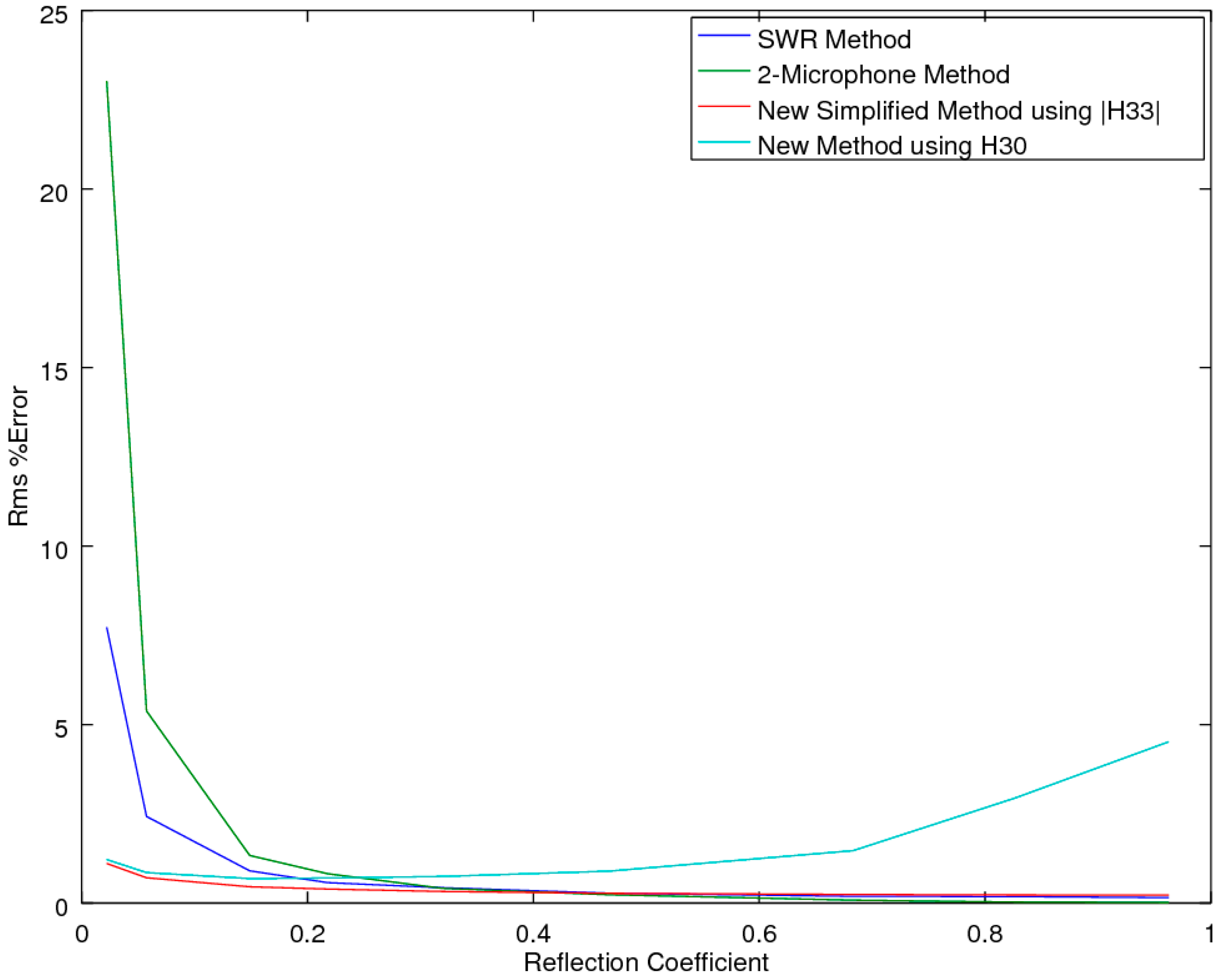
In examining the results, shown in Figure 5, Figure 6 and Figure 7, of interest is that both standard methods (SWR [2] and the two-microphone method [5,6]) exhibited excellent performance for highly reflective samples (R > 0.5). However, as the signal level dropped, due to the sample absorbing a lot of energy, the performance became increasingly poorer. Contrarily, the new proposed CSMM method, using H30, exhibited much better performance for highly reflective samples, but then faltered as the absorption decreased. It was especially poor for low values of β. Of particular interest, however, is the uniformly strong performance provided by the SSMM method that utilizes the |H33| transfer function by which to measure R. Out of all the methods, the SSMM technique proved to be the most robust estimator when presented with a real signal that included noise.
3.2. Accuracy Comparison for Online System
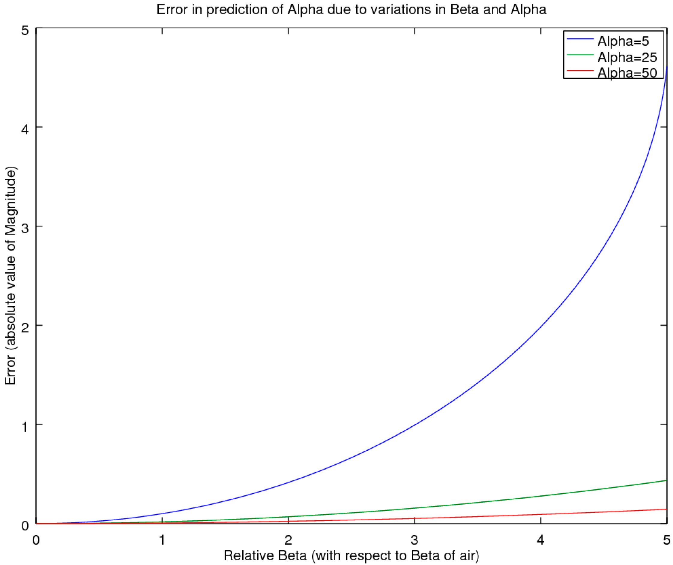
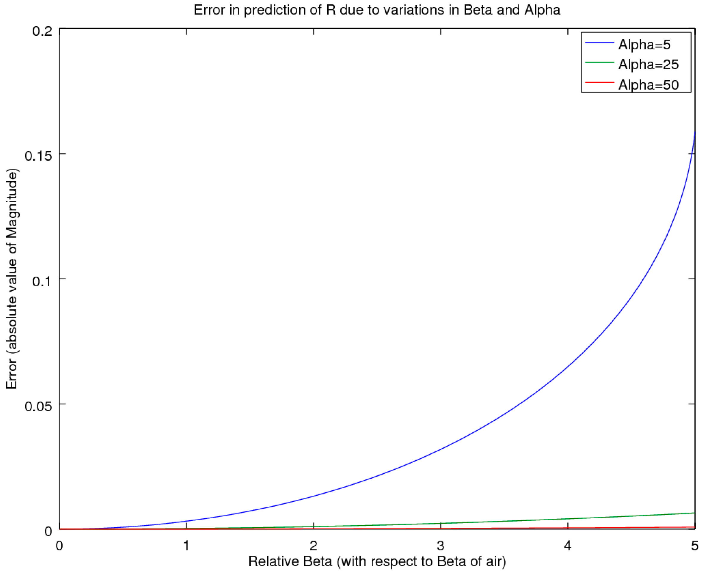
For devices that must operate online, the use of a periodic air-reference can be problematic. Further, as capturing phase information increases the complexity of the solution, hence a version that only utilizes pressure-magnitude measurements that can be self-calibrating and performed online is of interest. This section examines the potential use for utilizing the CSMM method with only pressure amplitudes (no phase), which would then utilize a magnitude |H30| transfer function. As this method was not derived from first principles, it was expected that errors would be present in comparison to the first-principle methods of the CSMM methodology. To examine the potential for this alternative simplified method, a simulation comparison was performed, whereby the material properties of the sample were allowed to vary across the full range expected from typical materials such as air, water, metals, wood, rubber cork and others, as reported in Beis and Hansen [19]. For most of these materials, the propagation velocity is higher than that of air, yielding a wave-number of β < 1, and in exception to these typical materials are a few unique materials such as cork and rubber, for which the maximum β is at most equal to 5. This then provided the bounds for the simulation study, whereby the values of α were allowed to range from very small, α = 5, to large, α > 200. Across this two-parameter variational boundary, the error was tracked and is presented in Figure 8 as the deviation for the measured α, and in Figure 9 as the deviation of measured R.
Looking at the magnitude of the error, shown in Figure 8 and Figure 9, across the range of β < 1 (which encompasses most materials for which the sonic velocity inside the material is greater than in air), we see that the error is inconsequential. For the more specialized case whereby sound velocity through the material was less than in air (1 < β < 5; which covers only a few specialized materials such as cork and rubber) we see that for most cases of α > 20, again the errors are reasonable. It is only for the case whereby the absorbance of the material was very low, α < 7, that the errors become significant. Pertinent to this very specialized situation is that this case would only apply to these materials if they were also low-performing acoustic materials; of the two such materials that the authors were aware of, cork and rubber, neither are poor absorbers and hence this criteria would not apply to them. Thus, as such, the authors are unaware of any materials that would fit into this category. Further, even for such a candidate, it is likely that this criterion would only be satisfied at low frequencies, as with increases in frequencies, a coincident increase in α is typical, which again would greatly alleviate the error to the point of inconsequence as the testing moved into the region for which the human auditory system is most sensitive. As such, these slow propagating-wave cases represent an unusual situation that will not be of concern to most practitioners. However, upon testing, should the users find themselves working with such an unusual material, the authors recommend setting up the instrumentation to also capture the phase to avoid these errors and fall back to the full CSMM method.
3.3. Experimental Confirmation
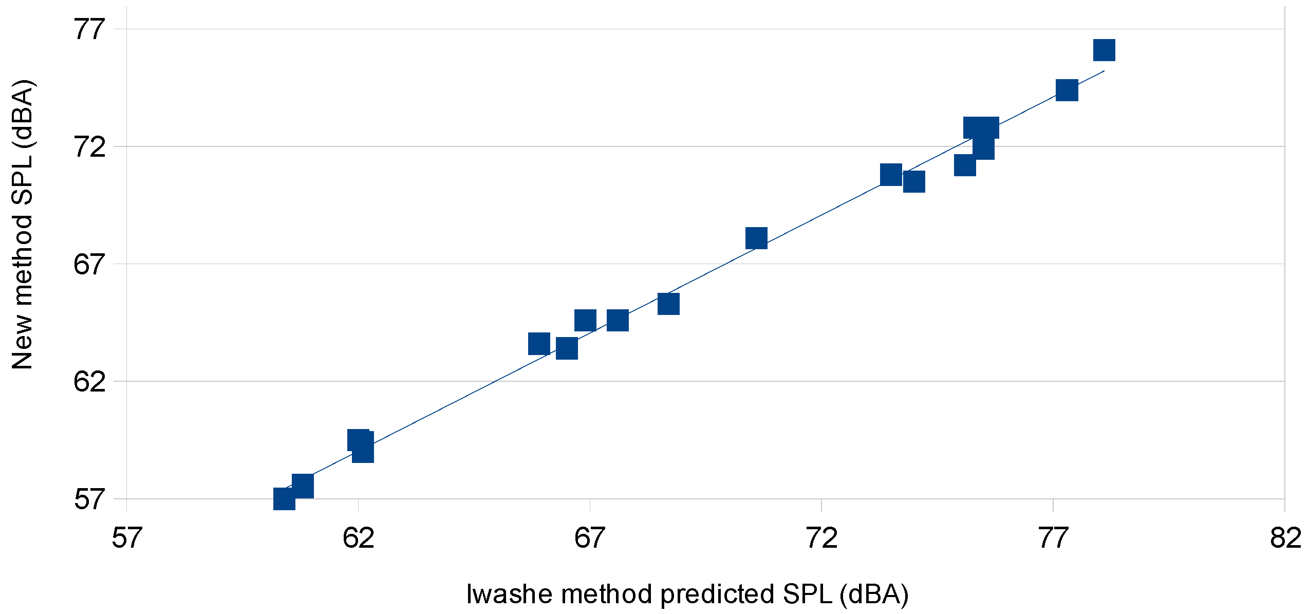
The experiments were analyzed and the spectral responses for each test specimen were reduced to a single value utilizing the A-weighted spectral reduction metric. The comparison of the A-weighted values between the new proposed SSMM |H33| method and the original Iwase method produced a very strong correlation, resulting in a coefficient of determination of r2 = 0.994. There was a minor small slope and offset bias. As such, in practice, for comparative studies utilizing only the new SSMM method, the near-perfect correlation provides strong supporting evidence for this methodology. Figure 10 details the regression analysis for how well the new formulation tracked the original Iwase [14] three-microphone method.
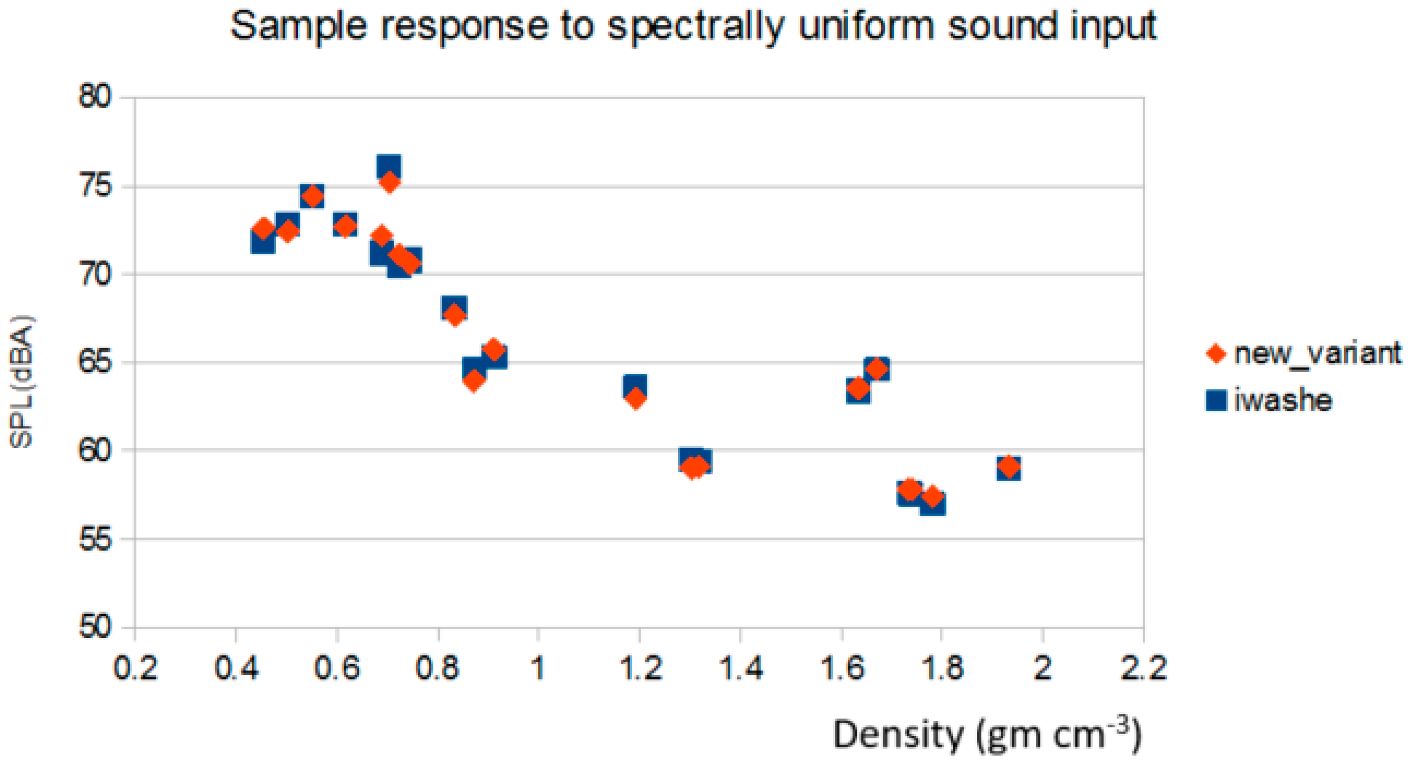
The next feature of interest is to ascertain how well the proposed SSMM method performs as the density varies. The comparison between the SSMM to the original Iwase [14] method was found to track well across the entire span of the wide range of densities tested. Figure 11 provides details in how the results compared between the two methods, as a function of density.
4. Discussion
In the theoretical section, the formulation for the SMM method was developed following the same approach as was utilized in the standard two-microphone method [5,6] and by Iwase et al. [14] in their derivation of the three-microphone method. The derivation of the SMM method predicted that if one is only interested in the through-transmission acoustic attenuation (loss), then the simplified SSMM method can be utilized, as it would require only a single microphone that is located on the far side of the sample at the reflection plate (no air gap). The performance of the experimental test section confirmed the predicted performance when utilized with an A-weighted metric response. The wide range of densities simulated and tested experimentally further confirms the SSMM technique can be utilized with confidence across a broad range of materials and applications.
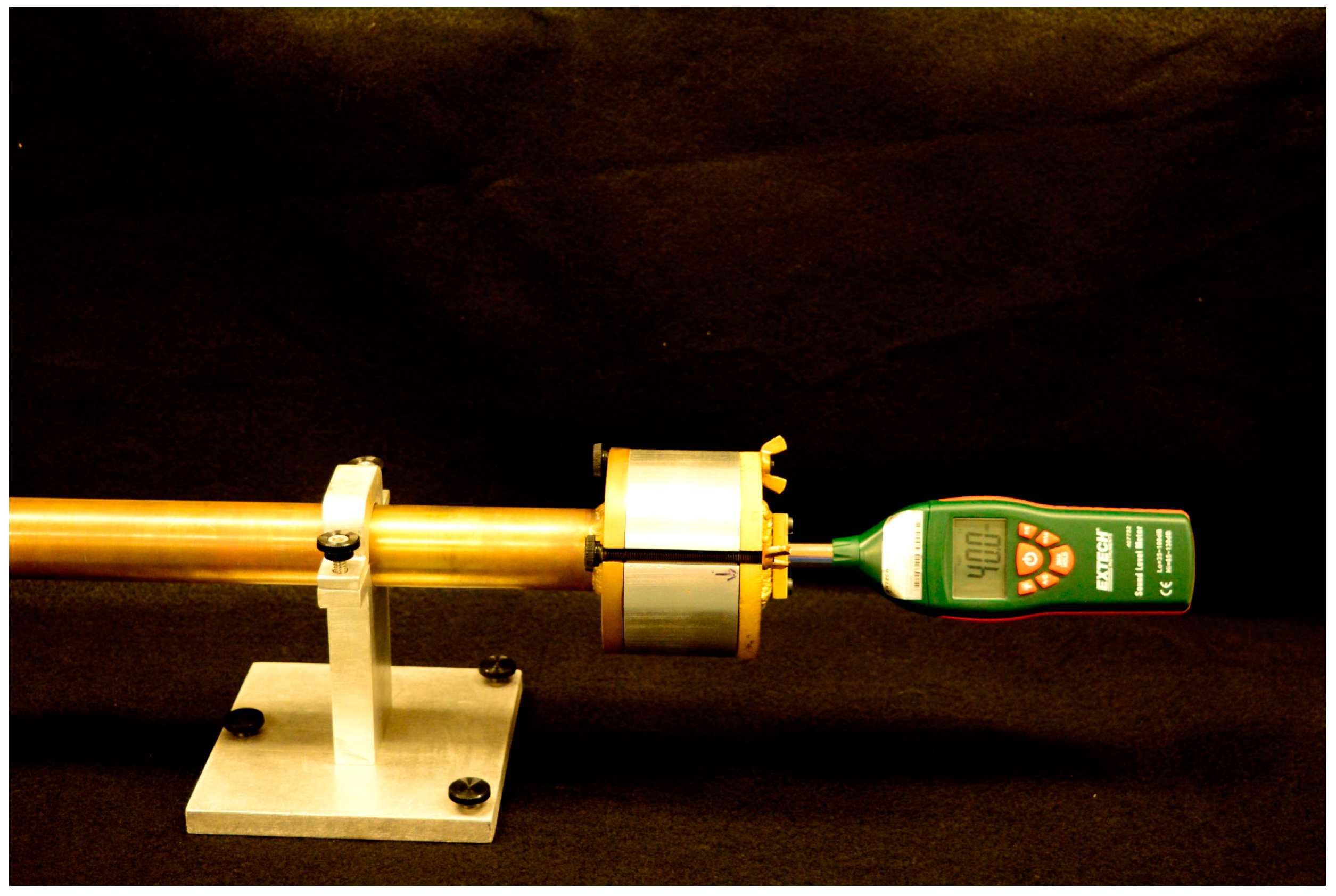
The SSMM method compares the results from an air test (no sample) measurement to the measurement that one obtains with the sample, and then utilizing Equations 12 and 14, allows for a prediction of the material propagation constant. Of note is that one of the primary benefits of obtaining the material propagation constant is that it is a measure of the material’s properties, and hence can be utilized to infer acoustic through-transmission attenuation for thinner or thicker samples, as desired. As such, one of the most notable features of the proposed SSMM method is that it does not require simultaneous measurements, and avoids the need for resolving the phase components of the complex propagation of the signals. Due to this fact, one can perform the SSMM method with greatly simplified instrumentation, requiring only a tube, a sample holder, sound-source, speaker/amplifier and a sound meter mounted in the reflection plate, which in this case, would significantly reduce the complexity, as it completely avoids the necessity for expensive microphones, microphone pre-amps, signal-capture instrumentation and complicated post-processing. Further, as the sound meter is already configured to an A-weighted acoustic response curve, all of the required processing is provided by the sound meter, thereby avoiding expensive and complicated software for the post-processing of the signals. For screening studies, the authors suggest the practitioner supplies a broadband white- or pink-noise amplified signal to the speaker. This reduction in complexity afforded by the new SSMM method is best illustrated by comparing the full system, shown in Figure 1, Figure 2 and Figure 3, to the simplified SSMM system that, when outfitted with a simple sound meter, reduces to just the tube, sound-level meter and sample holder, as shown in Figure 12.
In examining the accuracy exposed by the simulation studies, there are a few noteworthy details that have not received much coverage in the literature. As such, it is instructive to note that while any of the methods can be practiced using mono-tone sample interrogation, in which case comparable results should be obtained, with the deviations due to normal experimental error sources, such as sample sealing and tube resonance as the dominant error sources, the methods can also be practiced using multi-frequency approaches that utilize white or pink-noise sources. In the case of broad-band signal captures, it is recommended for high accuracy applications to utilize coherent noise-sources and to also capture the phase information. Of interest for phase capture is that the incoming audio signal can be utilized as a reference; thereby preserving the need for only a single microphone. Of importance to note is that the SMM methods proposed here have an additional advantage over the other methods when configured to utilize only a single microphone; hence there are no errors associated with comparing readings between two different microphones, which avoids the entire microphone gain-phase calibration process and its subsequent errors. Additionally, as the reference reading can be stored and does not drift greatly in standard temperature and pressure laboratories, the technique really is a single-measurement method, with a few reference readings required only at periodic intervals to ensure it has not drifted. In many respects, the SSMM, using the |H33| transfer function, is similar to running spectroscopy samples whereby a blank reference sample is periodically run. As such, it provides the accuracy of the one-microphone method utilized for the two- and four-microphone methods, where the microphone is physically moved between readings, while avoiding the burden of physically moving the microphone, which is tedious and time-consuming. Hence, if this method is automated utilizing the mono-frequency approach, it provides enhanced accuracies over the afore-mentioned methods, and can obtain a scan in a relatively short duration of 1–5 s, depending upon the integration times selected to reduce noise levels in the measurements.
For the highest accuracy measurements, the use of a mono-frequency generator is suggested. While it is possible to speed up data-acquisition using multiple frequencies and performing the analysis utilizing frequency separation and filtering afforded by techniques such as the discrete Fourier transform, in practice, the time savings are minimal, as the bulk of the time is not spent in the data-collection phase, but is predominantly comprised of the time required to carefully seal the edges of the sample, along with the insertion and re-assembly of the sample chamber into the sample tube. As noted in Figure 5, Figure 6 and Figure 7, the SSMM method, using the H33 transfer function, with relative-phase capture, is expected to outperform the standard methods for samples with low reflectance properties, and should be the method of choice for these materials, circumstances of the application permitting.
5. Conclusions
This research introduced several new simplified variants of the standard acoustic test methods: the two-microphone [5,6] and Iwase three-microphone methods [14]. The new simplified methods presented herein, the CSMM and the SSMM methods, were derived from first principles, so as such, they both provide mathematical identities to the two- and three-microphone methods. As such, it was expected that they would provide comparable results to the original methods. To test this hypothesis, a comparative study was conducted utilizing both experimental data and a simulation analysis utilizing a Monte-Carlo approach to examine the comparative performance of the CSMM and SSMM methods when placed into a noisy environment. The results of the study revealed that the SSMM method was shown to provide distinct advantages (Figure 7) versus the standard two- and three-microphone methods [5,6,14] when operating in a noisy environment. As such, this is the author’s recommended method for high-accuracy work, as it provides distinct advantages, especially when dealing with highly absorptive samples.
The experimental studies examined the performance of the SSMM method in comparison to the results produced by the original Iwase three-microphone technique [14]. The testing was conducted across a wide variety of samples, thereby providing a large span in sample density and material absorptive properties. A correlation analysis between the two methods was conducted, utilizing the A-weighted spectral reduction metric as the analysis variable for the regression study. The coefficient of determination between the two methods produced r2 = 0.994 (Figure 10 and Figure 11).
The combination of the theoretical derivation coupled with the simulation study and experimentally obtained strong correlation across such a wide range in densities provided convincing evidence that the SSMM method should be a candidate for any new test facility looking to add acoustic test capabilities to their laboratory’s curriculum. Noting that the proposed method only requires measurement of the amplitude signal at the end of the impedance tube, the experimental requirements can be reduced to only the tube, a speaker and a single sound meter (Figure 12), which eliminates the requirement for numerous expensive instrument microphones, their associated microphone pre-amplifiers, high-speed simultaneous sampling data-acquisition systems and elaborate computational software. This simplification, provided by the new proposed SSMM test method, results in significant reductions in equipment costs and expertise that is required to run acoustical test studies.
Acknowledgments
Special thanks to the team at Ecovative Designs for the materials and services provided.
Author Contributions
Mathew G. Pelletier, John D. Wanjura and Greg A. Holt conceived and designed the experiments, analyzed the data and wrote the paper.
Conflicts of Interest
The authors declare no conflict of interest.
Disclaimer
Mention of product or trade name does not constitute any endorsement by the USDA-ARS over other comparable products. Products and companies are listed for reference only. USDA is an equal opportunity provider and employer.
References
- Seybert, A.F.; Ross, D.F. Experimental determination of acoustic properties using a two-microphone technology random-excitation. J. Acoust. Soc. Am. 1977, 61, 1362–1370. [Google Scholar] [CrossRef]
- International Organization for Standardization (ISO) 10534-1. Acoustics–Determination of Sound Absorption Coefficient and Impedance in Impedance Tubes–Part 1: Method Using Standing Wave Ratio, International Organization for Standardization: Geneva, Switzerland, 1996.
- Chung, J.Y.; Blaser, D.A. Transfer function method of measuring in-duct acoustic properties. I. Theory. J. Acoust. Soc. Am. 1980, 68, 907–913. [Google Scholar] [CrossRef]
- Chung, J.Y.; Blaser, D.A. Transfer function method of measuring in-duct acoustic properties. II. Experiment. J. Acoust. Soc. Am. 1980, 68, 914–931. [Google Scholar] [CrossRef]
- American Society of Testing Materials (ASTM) E1050. Standard Test Method for Impedance and Absorption of Acoustical Materials Using a Tube, Two Microphone and a Digital Frequency Analysis System, ASTM International: West Conshohocken, PA, USA, 2010.
- International Organization for Standardization (ISO) 10534-2. Acoustics–Determination of Sound Absorption Coefficient and Impedance in Impedance Tubes–Part 2: Transfer Function Method, International Organization for Standardization: Geneva, Switzerland, 1998.
- Doutres, O.; Salissou, Y.; Atalla, N.; Panneton, R. Evaluation of the acoustic and non-acoustic properties of sound absorbing materials using a three-microphone impedance tube. Appl. Acoust. 2010, 71, 506–509. [Google Scholar] [CrossRef]
- Salissou, Y.; Panneton, R. Wideband characterization of the complex wave number and characteristic impedance of sound absorbers. J. Acoust. Soc. Am. 2010, 128, 2868–2876. [Google Scholar] [CrossRef] [PubMed]
- Wolkesson, M. Evaluation of Impedance Tube Methods–A Two Microphone In-Situ Method for Road Surfaces and the Three Microphone Transfer Function Method for Porous Materials. Master’s Thesis, Chalmer’s University of Technology, Goteborg, Sweden, 2013. [Google Scholar]
- American Society of Testing Materials (ASTM) E2611. Standard Test Method for Measurement of Normal Incidence Sound Transmission of Acoustical Materials Based on the Transfer Matrix Method, ASTM International: West Conshohocken, PA, USA, 2009.
- Bolton, J.S.; Hou, K. Calibration methods for four-microphone standing wave tubes. In Proceedings of the 23rd National Conference on Noise Control Engineering, NOISE-CON, Dearborn, MI, USA, 28–31 July 2008; pp. 1112–1120. [Google Scholar]
- Cox, T.J.; D’Antonio, P. Acoustic Absorbers and Diffusers: Theory, Design and Application, 2nd ed.; Taylor & Francis: New York, NY, USA, 2009; pp. 17–21, 100–101. [Google Scholar]
- Song, B.H.; Bolton, J.S. A transfer-matrix approach for estimating the characteristic impedance and wave numbers of limp and rigid porous materials. J. Acoust. Soc. Am. 2000, 107, 1131–1152. [Google Scholar] [CrossRef] [PubMed]
- Iwase, T.; Izumi, Y.; Kawabata, R. A new measuring method for sound propagation constant by using sound tube without an air spaces back of a test material. In Proceedings of the 1998 International Congress on Noise Control Engineering, Christchurch, New Zealand, 16–18 November 1998; New Zealand Acoustical Society: Christchurch, New Zealand, 1998. [Google Scholar]
- D’astrous, F.T.; Foster, F.S. Frequency dependence of ultrasound attenuation and backscatter in breast tissue. Ultrasound Med. Biol. 1986, 12, 795–808. [Google Scholar]
- Szabo, T.L. Time domain wave equations for lossy media obeying a frequency power law. J. Acoust. Soc. Am. 1994, 96, 491–500. [Google Scholar] [CrossRef]
- Chen, W.; Holm, S. Modified Szabo’s wave equation models for lossy media obeying frequency power law. J. Acoust. Soc. Am. 2003, 114, 2570–2574. [Google Scholar] [CrossRef] [PubMed]
- Pritz, T. Frequency power law of material damping. Appl. Acoust. 2004, 65, 1027–1036. [Google Scholar] [CrossRef]
- Beis, D.A.; Hansen, C.H. Engineering Noise Control, 4th ed.; Taylor and Francis Group: New York, NY, USA, 2009; pp. 318–321. [Google Scholar]
- Niresh, J.; Neelakrishnam, S.; Subha Rani, S. Investigation and correction of error in impedance tube using intelligent techniques. J. Appl. Res. Technol. 2016, 14, 405–414. [Google Scholar] [CrossRef]
Figure 1.
Schematic diagram of the experimental apparatus detailing the testing configuration for performing the standard two-microphone method, the 1998 three-microphone method of Iwase et al., to obtain complex material propagation coefficients.
Figure 1.
Schematic diagram of the experimental apparatus detailing the testing configuration for performing the standard two-microphone method, the 1998 three-microphone method of Iwase et al., to obtain complex material propagation coefficients.

Figure 2.
Picture showing the test apparatus utilized in the study. The apparatus has multiple upstream microphones for performing ISO 10534-2 as well as an insertion traveling microphone, attached to the cable seen entering the tube just to the right of the speaker on the far left of the tube. Seen on the far right of the tube is the silver aluminum sample holder that has a microphone embedded into the side wall to perform the sample surface pressure measurement: Iwase [12] microphone 0. At the far right is Iwase [12] transmission microphone 3 that is embedded in the end reflection-plate.
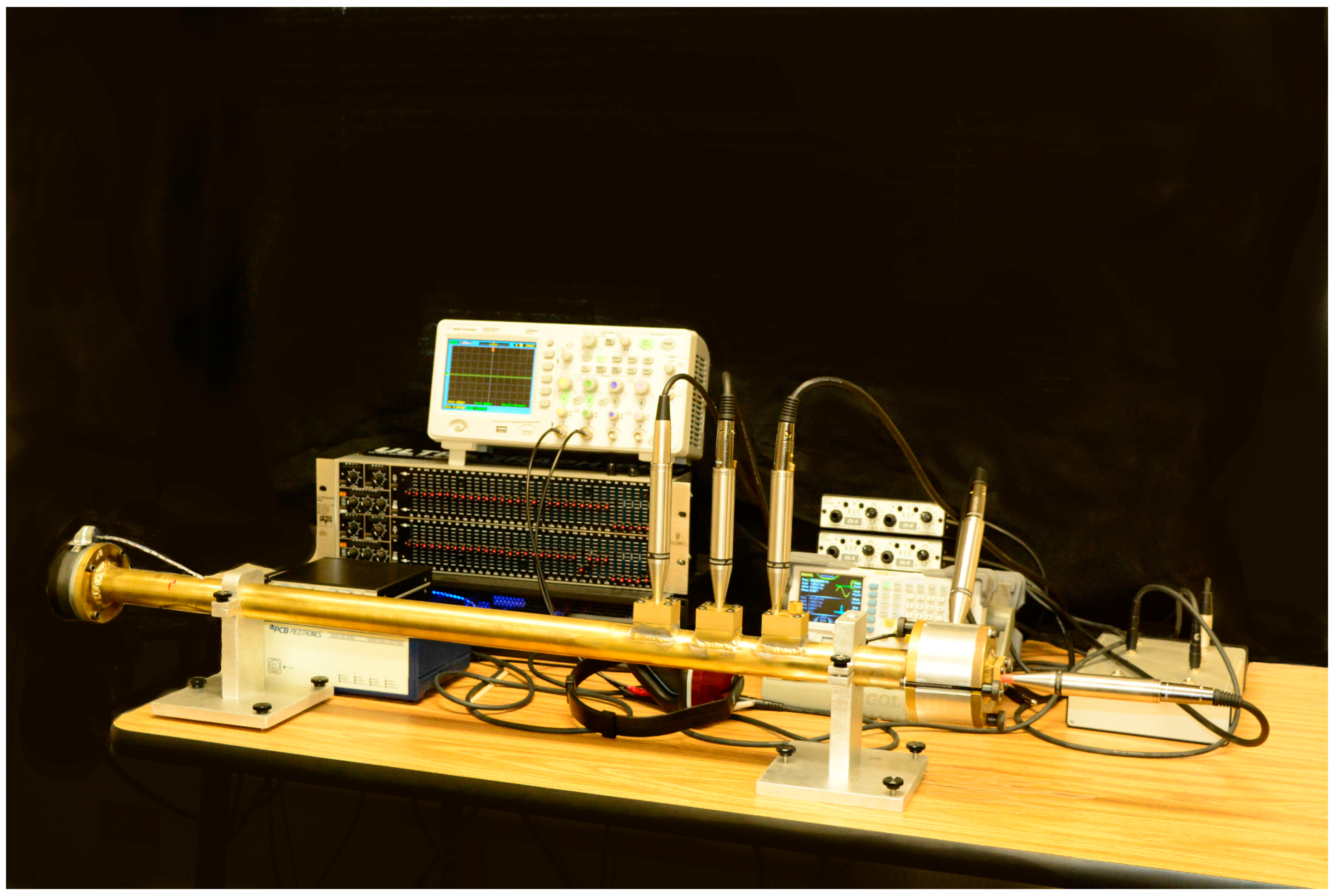
Figure 3.
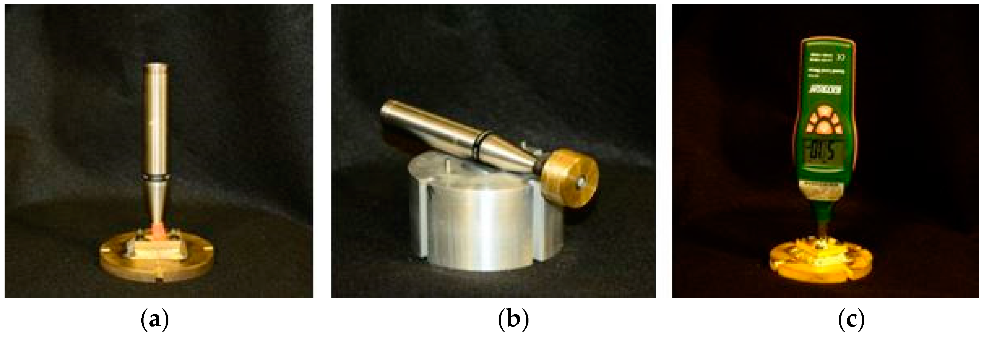
Picture showing the various instrumented end plates for the experimental test apparatus utilized in the study. Each of these end plates provided a different means to obtain the Iwase [12] microphone 3 measurements. The image (a) on the left shows a microphone embedded into the end reflection plate. In the middle image (b) is the sample holder as well as an instrumented movable piston-style reflection plate. The piston configuration allowed for easy adjustment of the reflection plate location. Seen on the far right in image (c) is a reflection plate with an NIST traceable A-weighted sound meter mounted in a pressure-tight sealed reflection plate. Option (c) provided the easiest method of the three, and provided the lowest-cost entry into acoustic testing.
Figure 3.
Picture showing the various instrumented end plates for the experimental test apparatus utilized in the study. Each of these end plates provided a different means to obtain the Iwase [12] microphone 3 measurements. The image (a) on the left shows a microphone embedded into the end reflection plate. In the middle image (b) is the sample holder as well as an instrumented movable piston-style reflection plate. The piston configuration allowed for easy adjustment of the reflection plate location. Seen on the far right in image (c) is a reflection plate with an NIST traceable A-weighted sound meter mounted in a pressure-tight sealed reflection plate. Option (c) provided the easiest method of the three, and provided the lowest-cost entry into acoustic testing.

Figure 4.
Comparison chart depicting pressure inside the tube with and without noise for two different reflection coefficients R. The large amplitude signal is the response when the sample’s R was 0.99. The low-amplitude signal is the response for a sample with a much lower R of 0.05. The frequency for this test case was 1000 Hz with a material-relative phase delay of β = 1.20.
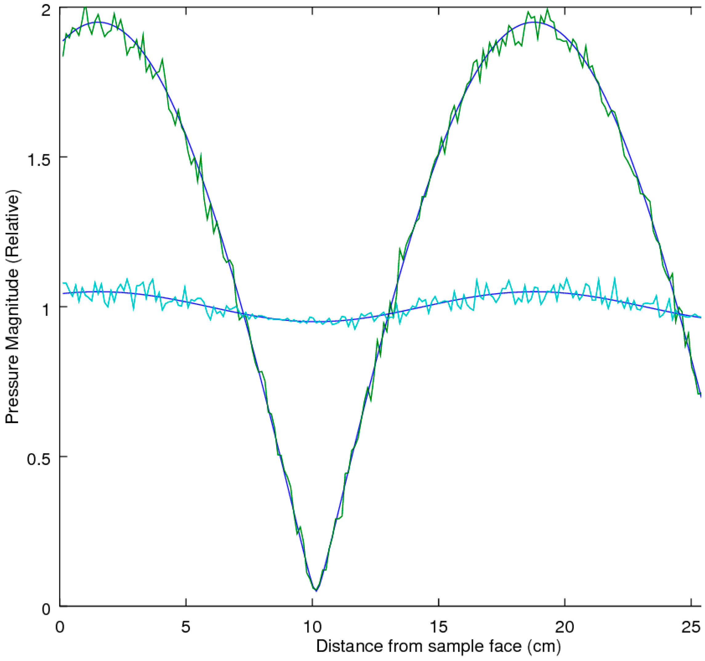
Figure 5.
Comparison of accuracy from the computation of R, with a normalized noise level of 0.005 and a β value of 0.1. Comparison is between the two standard methods, SWR [2] and the two-microphone method [5,6], and the technique utilized in the three-microphone method [14], versus the new proposed methods utilizing the simplified |H33| method (amplitude only measurements) and the technique that uses a measurement of H30 (complex measurements that include phase relationships).

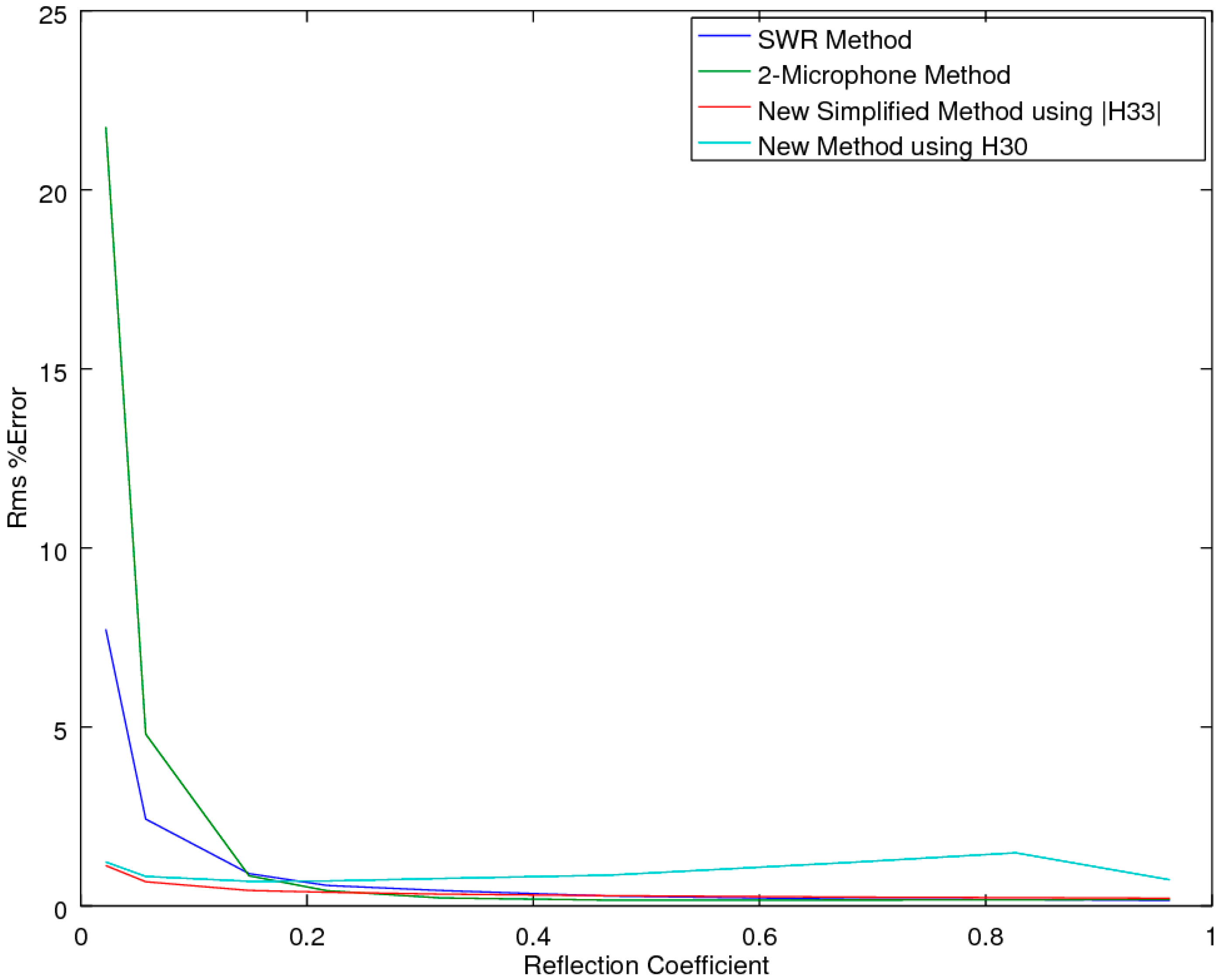
Figure 6.
Comparison of accuracy from the computation of R, with a normalized noise level of 0.005 and a β value of 2.0. Comparison is between the two standard methods, SWR [2] and the two-microphone method [5,6], and the technique utilized in the three-microphone method [14], versus the new proposed methods utilizing the simplified |H33| method (amplitude only measurements) and the technique that uses a measurement of H30 (complex measurements that include phase relationships).
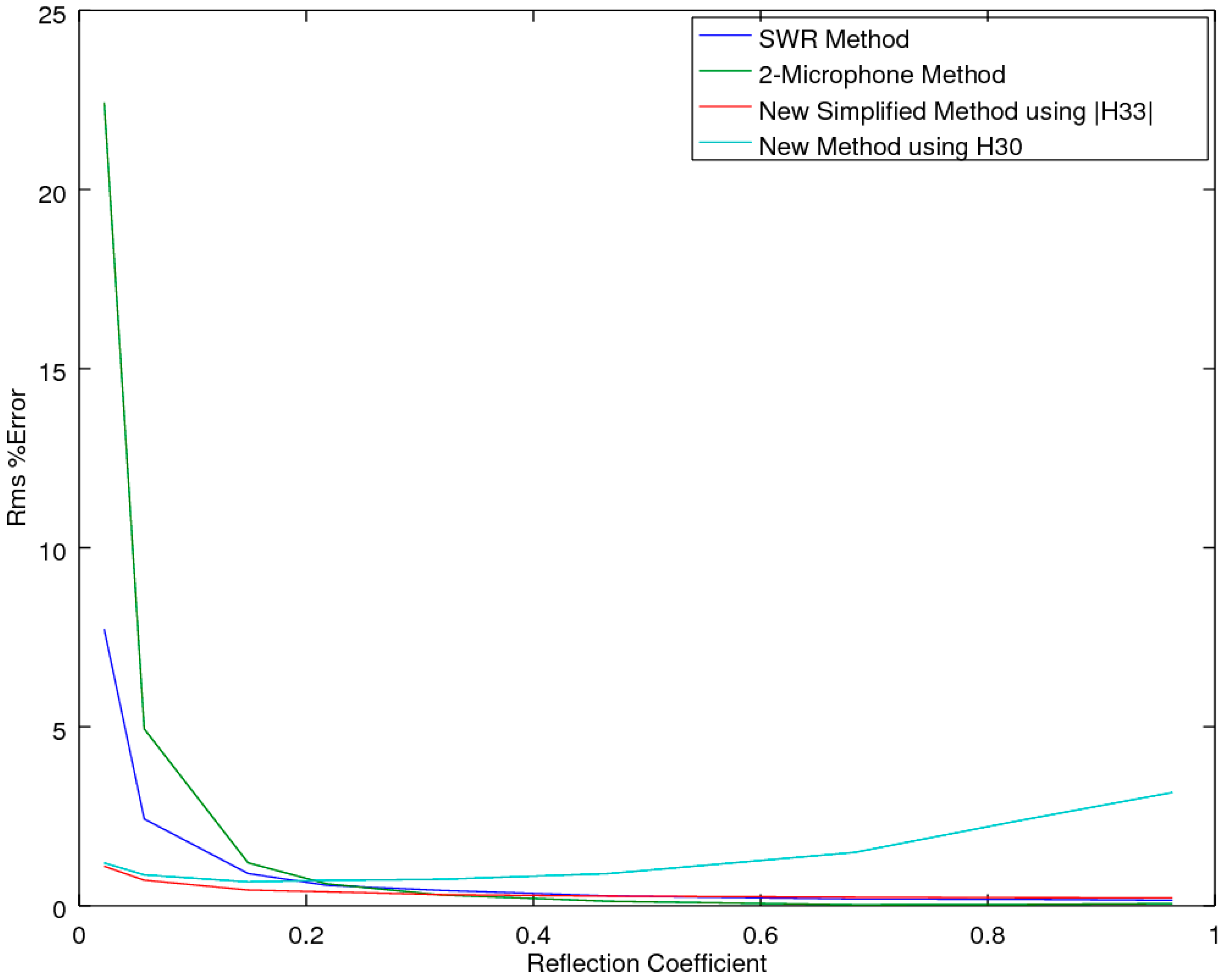
Figure 7.
Comparison of accuracy from the computation of R, with a normalized noise level of 0.005 and a β value of 5.25. Comparison is between the two standard methods, SWR [2] and the two-microphone method [5,6], and the technique utilized in the three-microphone method [14], versus the new proposed methods utilizing the simplified |H33| method (amplitude only measurements) and the technique that uses a measurement of H30 (complex measurements that include phase relationships).

Figure 8.
Error comparison for the CSMM simplified new method utilizing only pressure-magnitude readings |H30|. Error is reported as the magnitude of the absolute value of the error of the predicted value of α. Error magnitude was computed as material propagation changes occurred for both α and β (typical materials have a propagation delay with relative β < 1).

Figure 9.
Error comparison for the CSMM simplified new method utilizing only pressure-magnitude readings |H30|. Error is reported as magnitude of the absolute value of the reflection coefficient R.
Figure 9.
Error comparison for the CSMM simplified new method utilizing only pressure-magnitude readings |H30|. Error is reported as magnitude of the absolute value of the reflection coefficient R.

Figure 10.
Correlation analysis for attenuation between A-weighted response, as measured utilizing the Iwase [12] three-microphone method, versus the new proposed SIM method.
Figure 10.
Correlation analysis for attenuation between A-weighted response, as measured utilizing the Iwase [12] three-microphone method, versus the new proposed SIM method.

Figure 11.
Shown above is a comparison graph for the Iwase [14] method versus the new proposed simplified SSMM method (after correction for bias and slope offset). The comparison utilizes the A-weighted spectral reduction metric to provide a single-valued comparison, from multi-frequency spectral data.

Figure 12.
Simplified acoustic testing equipment setup that is enabled through the use of the SIM method.
Figure 12.
Simplified acoustic testing equipment setup that is enabled through the use of the SIM method.

© 2017 by the authors. Licensee MDPI, Basel, Switzerland. This article is an open access article distributed under the terms and conditions of the Creative Commons Attribution (CC BY) license (http://creativecommons.org/licenses/by/4.0/).
Share and Cite
MDPI and ACS Style
Pelletier, M.G.; Holt, G.A.; Wanjura, J.D. Simplified Three-Microphone Acoustic Test Method. Instruments 2017, 1, 4. https://doi.org/10.3390/instruments1010004
AMA Style
Pelletier MG, Holt GA, Wanjura JD. Simplified Three-Microphone Acoustic Test Method. Instruments. 2017; 1(1):4. https://doi.org/10.3390/instruments1010004
Chicago/Turabian StylePelletier, Mathew G., Greg A. Holt, and John D. Wanjura. 2017. "Simplified Three-Microphone Acoustic Test Method" Instruments 1, no. 1: 4. https://doi.org/10.3390/instruments1010004