Universal Signal Conditioning Technique for Fiber Bragg Grating Sensors in PLC and SCADA Applications


1
School of Biomedical Sciences, The University of Western Australia, Perth, WA 6009, Australia
2
School of Engineering, RMIT University, Melbourne, VIC 3053, Australia
3
School of Science, Edith Cowan University, Perth, WA 6027, Australia
4
Centre for Communications and Electronics Research (CCER), School of Engineering, Edith Cowan University, Perth, WA 6027, Australia
*
Author to whom correspondence should be addressed.
Instruments 2017, 1(1), 7; https://doi.org/10.3390/instruments1010007
Submission received: 2 October 2017
/
Revised: 20 November 2017
/
Accepted: 4 December 2017
/
Published: 7 December 2017
Abstract
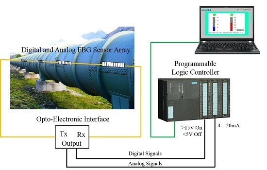
:Optical fibre sensors, such as Fibre Bragg Gratings (FBGs), are growing in their utilisation, although very niche in their applications. To enable a more diverse range of end users, expensive application-specific optical fibre interrogation hardware needs to be made compatible with and, ideally, easily incorporated into existing instrumentation and measurement hardware. The Programmable Logic Controller (PLC) is an ideal example of hardware used for data acquisition in many industries. As such, a module that can be connected into an existing PLC slot to collect data from electrically-neutral, EMI-immune and versatile FBG sensors is of significant advantage to the growing optical fibre sensing market. In this work, we show that both digital and analogue signals can be collected from FBG sensors and integrated seamlessly into the PLC-based control system using a transmit-reflect detection system. This technique enables fibre optic sensors to be compatible with standard industrial automation controllers in a relatively low cost and plug and play manner.
1. Introduction
Programmable Logic Controllers (PLCs) are the standard intelligence for instrumentation and control systems utilised in process control and are used in a wide variety of industries from car manufacturing to building management systems, as well as controlling machinery in large mine sites [1]. PLCs often form the basis of many automated industrial processes and are essentially the heart of a Supervisory Control And Data Acquisition (SCADA) system. A PLC is an electro-mechanical computer specifically designed to take in information from a multitude of sensors in real-world industrial processes and react to those sensing inputs by controlling actuators in such a way as defined by the control logic [2]. For example, a PLC may receive data corresponding to the pressure of a fluid in a pipeline and then react to that signal by sending a command to the field to open a valve, stop a pump, sound an alarm, or any other action, depending on what is required. Currently, there is a number of different communication protocols and sensing standards for automated processes, such as Profibus [3] and Foundation Fieldbus [4], as well as an array of smaller proprietary protocols. The particular standards used in any one process depend on a number of factors, from the size of the plant to the scale of automation required and the PLC manufacturer. One of the traditional analogue input sensing standards is 4–20 mA [5]. The physical signal from an analogue sensor to the PLC is between 4 mA and 20 mA, where 4 mA corresponds to 0% and 20 mA corresponds to 100% of the measurand. The main advantage of using this technique is that a faulty connection can be detected easily, as it will result in the PLC receiving 0 mA.
As with PLCs, optical fibre sensors are now used in a large variety of diverse applications and are capable of measuring many different types of signals, both static and dynamic, including temperature, pressure, level and flow, as well as chemical and biological measurands [6,7,8]. It is well recognized that optical fibre sensors have many desirable attributes, which are advantageous with respect to other sensing methodologies, which include greater sensitivity, reduced size and weight and immunity to electromagnetic interference. However, in general, optical fibre sensors are underutilised in process control applications. There are a number of reasons for this lack of penetration into mainstream industrial processes. These include the cost and complexity of optical fibre-based sensing systems, as well as the fact that simpler traditional sensing techniques based on well-established industrial standards are, to date, usually preferred. The use of optical fibre systems is increasing in some industrial applications, for both information transmission and sensing, since these systems are immune to electromagnetic interference and offer faster data transmission rates [9]. It has been proposed that signals from optical fibre sensors used in real-time industrial applications could be monitored with PLCs [10]. However, whilst most major PLC manufacturers now offer an optical fibre interface for communications, they do not enable optical fibre sensors to be connected directly to PLC I/O cards.
Where fibre optic sensors are used in process control applications, the sensors are usually on the end of an optical fibre, where the fibre is simply used as the data transmission medium. This method completely underutilizes many of the advantages of the fibre itself. A signal conditioning system was demonstrated however for optically identical Fabry-Perot sensors, capable of detecting different measurands in industrial applications [11]. Fibre Bragg Grating (FBG) sensors are also optical fibre-based sensors that have the advantage of being able to be multiplexed and hence can form a distributed sensing network, rather than a single sensor on the end of a line. Some of the multiplexing architectures are described in [12]. FBG sensors were first reported by Morey, Meltz and Glenn in 1989 [13], but they became widely accessible, after they demonstrated their transverse holographic fabrication method for FBGs [14]. Initially, FBGs were used as spectral transduction elements, whereby the sensing information corresponded directly to the wavelength shift of the FBG. As such, they can be implemented in Wavelength Division Multiplexing (WDM) or Time Division Multiplexing (TDM) systems [15]. Unfortunately, these systems require spectral decoding of the sensor signals, which can be costly and processor intensive.
A more efficient alternative is to use FBGs in an intensity-based detection system where the relative spectral shift in the FBG filter results in an optical power change, which in turn correlates with a change in the measurand [16]. This relatively simple interrogation technique can be used to convert the change in the measurand from the optical domain to the electrical domain, meaning they can easily be integrated into existing control system architectures without the need for expensive stand-alone optical interrogators. The disadvantage of intensity-based detection systems is that input optical power fluctuations are introduced. However, the simplicity of the interrogation of the signal and the reduced cost greatly outweigh the corresponding disadvantages in certain low frequency applications, such as in the process control industry.
Here, we show that the output from both digital and analogue optical fibre sensors can be interfaced with a PLC I/O rack. The output from an FBG-based optical switch can be interfaced with a digital input card on a PLC, and the output from a FBG temperature sensor can be interfaced to a standard 4–20 mA analogue input card on a PLC. This technique enables optical fibre sensors to be directly compatible with current industry standards for PLC systems.
2. Theory
2.1. Fibre Bragg Grating Fundamentals
FBGs [17,18] are discrete spectrally-reflective components that are written into the core of an optical fibre using a high intensity light source and a phase mask to create alternating regions of different refractive indices. The difference in refractive indices results in Fresnel reflection at each interface, and the regular period of the grating, , results in constructive interference in the reflection at a specific wavelength, called the Bragg wavelength, , which is given by,
where is the effective refractive index of the grating for the guided mode and is the grating period.
Any external environmental disturbance that causes a change in the refractive index or period of the grating results in a change in the Bragg wavelength and as such can be detected by an FBG. The change in Bragg wavelength as a function of induced strain, , is given by [19]:
where and are the strain-optic coefficients, is Poisson’s ratio and is the thermo- expansion coefficient.
2.2. Edge Filter and Power Detection
There are many different interrogation techniques [20] used to detect the change in Bragg wavelength shift due to an external measurand and convert it from the optical domain into the electrical domain. One of the simplest ways to detect a change in the Bragg wavelength is to transpose the shift into the optical power. In other words, rather than trying to measure a shift in the wavelength directly, convert the shift into a power change, which can easily be detected using a photoreceiver or optical power meter. Edge filter detection [21] is one of the simplest techniques and hence one of the most cost effective. In edge filter detection methods, the shift in the FBG spectrum is detected by use of a spectrally-dependent filter, which results in a change in intensity at the detector. The FBG is illuminated by a broadband source, such as a Superluminescent Diode (SLD). As the Bragg wavelength spectrum of the FBG shifts across the filter, it causes the transmitted intensity to vary as the filter’s transmittance varies as a function of wavelength.
In power detection methods [16], the shift in the FBG wavelength is detected by using a spectrally-dependent source, which results in a change of intensity at the detector. There are two power detection methods, linear edge source and the narrow bandwidth source. In narrow bandwidth source-based power detection [16], the laser source is centred about the 3-dB point of an FBG that is then intensity modulated by the strain-induced wavelength shift. That is, the reflected optical power is varied as the linear edge of the FBG is shifted in the spectrum. Either the reflected component or the transmitted component from the FBG can be used.
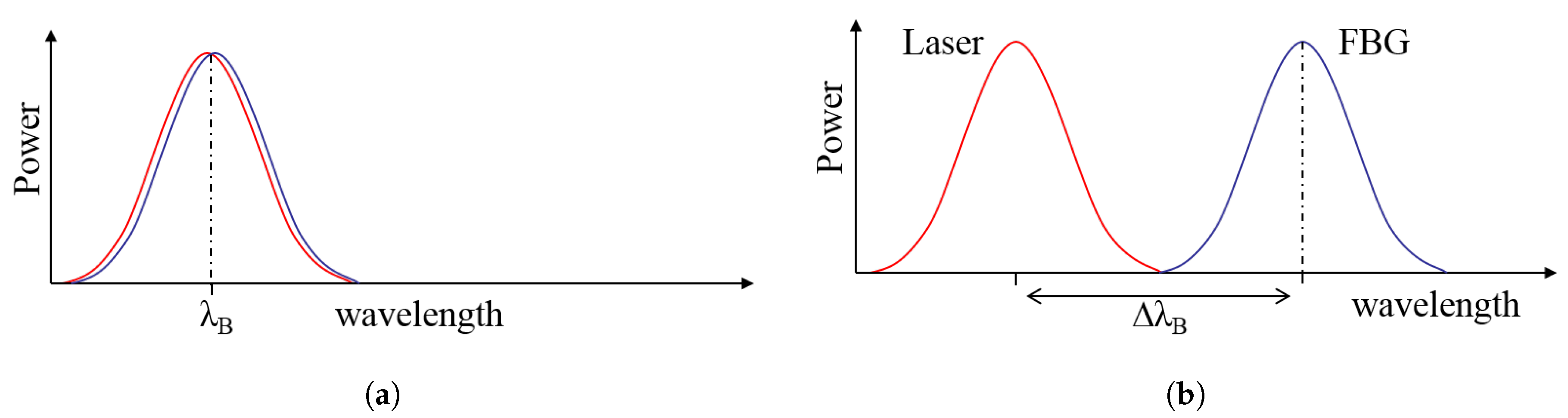
Power detection can be used to create an optical switch by optically mismatching an FBG with the laser source. When the Bragg wavelength and the laser wavelength are mismatched, the output is off. An external influence can be used to shift the Bragg wavelength so that the signals overlap, resulting in an on signal. Figure 1 shows the principle of operation of this type of optical switch.
2.3. Transmit Reflect Detection
In transmit-reflect detection methods, both the transmitted and reflected components occur simultaneously. As the Bragg wavelength of the FBG shifts due to an external measurand, the FBGs’ 3-dB point is also shifted. For a light source tuned to the 3-dB point, the amount of optical power reflected from (and transmitted through) the FBG will therefore change, either positive or negative, depending on which edge of the FBG was used, as the measurand varies. Since the transmitted and reflected components vary in opposite directions, they can be differentially amplified to increase the overall signal. It has been previously demonstrated that there are advantages associated with the use of both ends, specifically redundancy [22]. This is essential in practical industry settings where cables may be cut. By using both ends, all sensors would still be accessible. Furthermore, by using both ends in a differential mechanism, there are SNR gains that can be freely achieved [23]. Figure 2 shows the principle of operation of transmit-reflect detection. A review of FBG sensors and interrogation techniques is given in [6].
3. PLC Fibre Optic Sensor Digital Input Interface
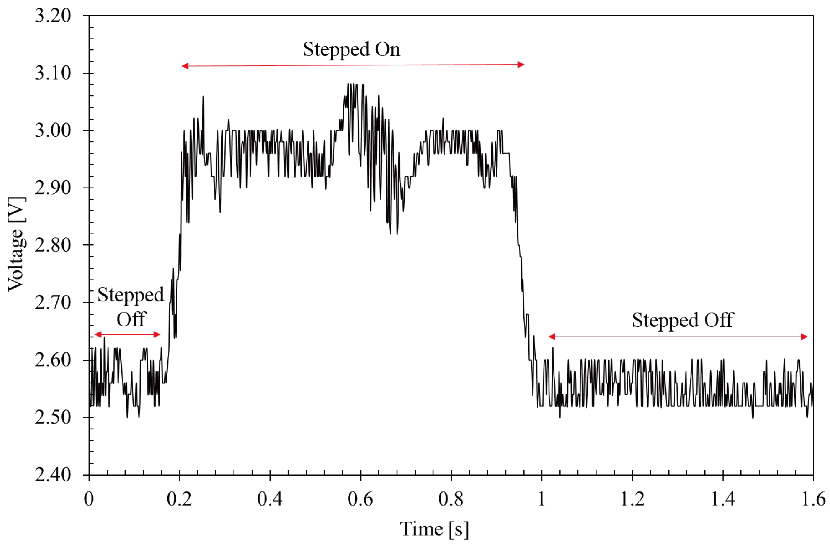
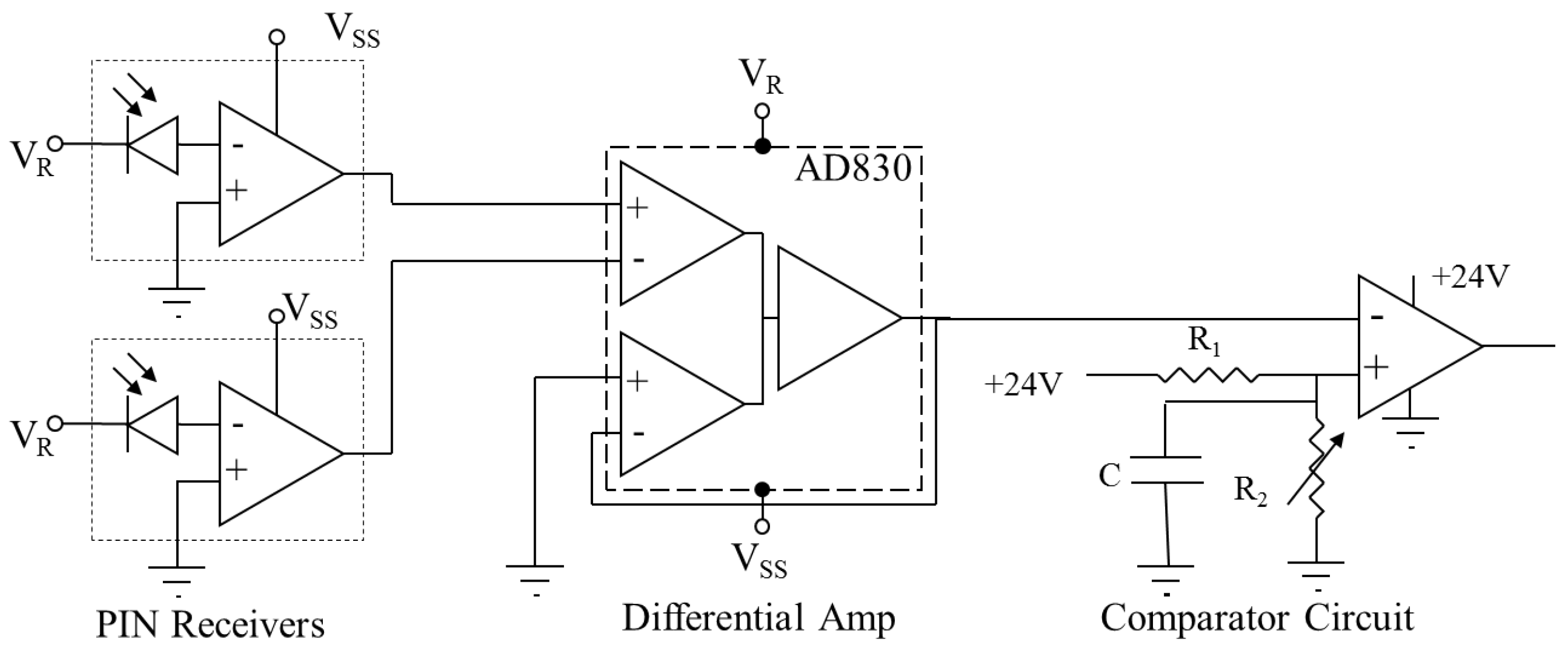
Here, a PLC Fibre Optic Sensor (FOS) digital input interface is demonstrated. An in-ground FBG pressure switch, previously reported in [24], whereby a 60-kg person stepped on a floorboard with the FBG bonded beneath it creating a voltage swing of approximately 0.5 V, was used as an arbitrary digital input signal for a PLC (Siemens S7-300, Munich, Germany). The Bragg wavelength of the FBG and the central wavelength of the laser were initially matched. As pressure was applied to the FBG, the Bragg wavelength shifted away from the laser’s position, producing an increase in transmitted optical power and a decrease in the reflected power, before returning back to its original position when it was stepped off.The PLC can be programmed to ensure the switch is latched on, so that the output alarm from the PLC would stay on until it is reset. As a PLC’s scan time is of the order of milliseconds, it would capture an increase in signal even if it then decreased.A bench-top tunable laser (Anritsu MG9637A, Kanagawa, Japan) was connected to the FBG (Micron Optics OS1100, Atlanta, GA, USA) via an optical circulator (FDK YC-1100-155, Tokyo, Japan). The reflected signal was directed down to the first photoreceiver (Fujitsu FRM3Z231KT, Tokyo, Japan) via the optical circulator, and the signal was transmitted through the FBG and was directed to the second receiver (Fujitsu FRM3Z231KT, Tokyo, Japan). The output of the two receivers was differentially amplified using a high speed differential amplifier (AD830ANZ, Norwood, MA, USA). The result is shown in Figure 3.
A simple comparator circuit was then used to ensure the differentially-amplified output voltage would be correctly interpreted by the PLC. The output from the comparator was then connected to a two-channel, 24-V digital input module on the I/O rack (Siemens ET200S, Munich, Germany). The digital input card detects a one when the input voltage is above 15 V, and it detects a zero when the input voltage is below 5 V. Hence, the 0.5-V swing, which occurred when the switch was stepped on was converted to a change of more than 10 V to ensure the value read by the PLC changed from a zero to a one. The transimpedance amplifier supply and the PIN bias for the two receivers was provided by a ±5-V DC power supply. The 24 V for the comparator circuit would be supplied by the PLC. The PLC FOS digital input interface circuit diagram is shown in Figure 4.
The in-ground pressure switch provided the digital signal for the PLC FOS digital input interface, which was connected to the digital input channel on the Siemens S7-300 PLC I/O rack. The experimental setup is shown in Figure 5.
4. PLC FOS Analogue Input Interface
Here, a PLC FOS analogue input interface is demonstrated. The experimental setup was similar to the previous setup, except a bench-top tunable laser module (Ando AQ 8201-13B, Tokyo, Japan) was used instead of the Anritsu MG9637A tunable laser. Again, the output of the two receivers was differentially amplified using a high speed differential amplifier (AD830ANZ, Norwood, MA, USA). An additional 3-V DC offset was supplied to the second summing input of the difference amplifier via a voltage divider from the +5 V. The DC offset was used due to the requirements of the transconductance amplifier. The transconductance amplifier converts a voltage range of 1 V–5 V into 4 mA–20 mA, as required by the PLC. This requires a bias resistance of 250 , giving 4 mA at 1 V and 20 mA at 5 V and, therefore, a midpoint of 3 V. The transimpedance amplifier (current-to-voltage converter) supply, PIN bias for the two receivers and the supply for the transconductance amplifier (voltage-to-current converter) was provided by a ±5 V DC power supply. Figure 7 shows the circuit diagram of the PLC FOS analogue input interface.
Initially, the spectral characteristics of the FBG needed to be measured, and the tunable laser needed to be set to the correct wavelength, in order to determine the operating point for the FBG sensor. The laser was initially tuned to the minimum reflectivity above the Bragg wavelength to ensure that all the optical power was transmitted through the FBG.
Prior to utilizing the optical input with the two transimpedance amplifiers, two function generators (Agilent 33250A, Santa Clara, CA, USA) were used, each set to give a negative voltage, similar to those expected from the transimpedance amplifiers. Initial tests showed the voltage of each receiver varied from −1 V–−2 V, for zero to maximum optical power (8 mW) of the tunable laser. The output of the difference amplifier was then between −1 V and 1 V, and with the 3-V offset, it then gave an expected 2 V–4 V output voltage to the transconductance amplifier, which corresponded to an expected output current of 8 mA–16 mA. To test the entire range of the system, the function generator output voltages were varied between −2.5 V and 0.5 V, to give an output current of 4 mA–20 mA, measured using a Digital Multimeter (DMM) (Goldstar DM-331, Seoul, Korea).
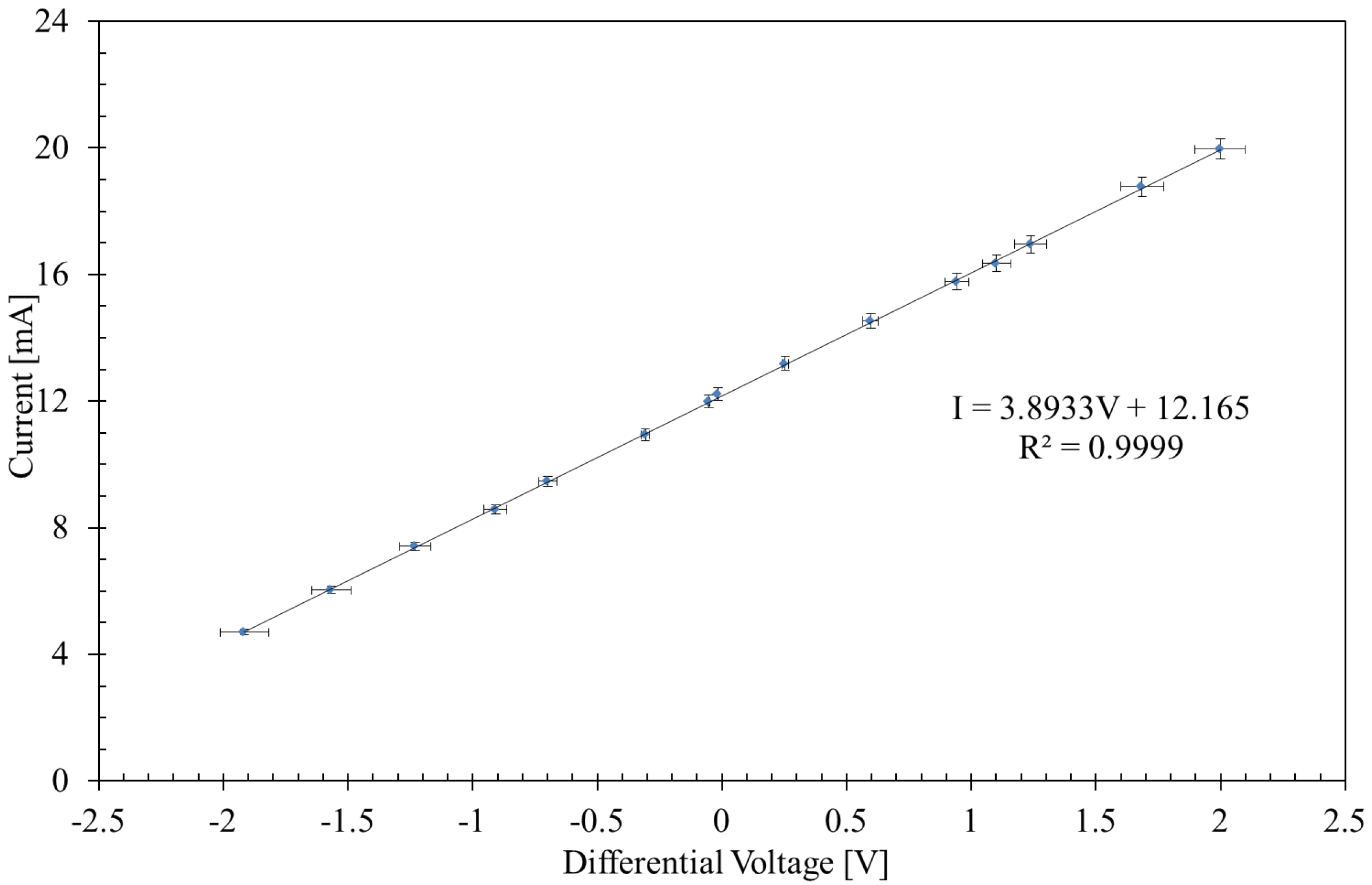
Figure 8 shows the transfer function of the transconductance amplifier. As shown, the transfer function is extremely linear, where the gradient is mA/V and the intercept is mA. There is a small discrepancy in the equation coefficient and offset, as we would expect the values for the gradient and intercept to be exactly 4 mA/V and 12 mA, respectively. The reason for this small inconsistency is most likely due to uncertainties in the voltage offset value, V, and the feedback resistance, , used in the transconductance amplifier circuit. Moreover, there is a small uncertainty in the precision of the DMM, mA and V, when measuring the current and voltage, respectively.
For the test experiment to monitor temperature, the FBG and a thermometer (Brannan 44/430/0, Cleator Moor, UK) were placed in a large beaker of water. The FBG was then connected to the optical circuit as before, and the water was then slowly heated using a hotplate (Industrial Equipment and Control PTY CH2093). The transmitted and reflected signals were connected to the optoelectronic PLC interface, and the output current was monitored on a DMM (Escort EDM168A, Santa Rosa, CA, USA) as a function of the temperature, before being connected to an analogue input channel on the Siemens S7-300 PLC I/O rack. The setup for the temperature measurement is show in Figure 9.
Figure 10 shows the output current from the complete circuit (Figure 7) as a function of the applied temperature to the FBG sensor. The curve is a sigmoid, or half a Gaussian, as we would expect. This is because both the laser and FBG are Gaussian in shape, and when multiplied together, the result is a Gaussian. The amplitude of this Gaussian increases from minimum to maximum. The optical power of the laser was such that the value of the voltage varied from minus 1.2 V to positive 0.2 V, corresponding to a change in current of approximately 6 mA, from 6.97 mA–12.81 mA. The asymmetry was due to the use of a temporary bare-fibre-connector, instead of a standard pigtail connector, adding more loss in the reflected path compared to the transmitted path. With the use of connectorised components, this would no longer be an issue. The straight line between 8.02 mA and 12.01 mA, where the gradient is mA/V and the intercept is mA, shows the region where the output current is linear with respect to temperature. Hence, in practice, this particular setup could be used as a temperature sensor with a range from approximately 22–30 C with higher precision than the thermometer used here, which had an uncertainty of ±0.5 C. A change of 0.1 mA detected by the PLC would be a result of a change in temperature of approximately 0.2 C.
The PLC was again programmed in ladder logic and a graphical representation of the input current to the PLC and the output temperature was created using WinCC Flexible software [25]. The direct readout from the analogue input module was converted into 4–20 mA, which was then converted into the actual temperature range, in the PLC logic. To achieve the conversion from current to temperature, the data from Figure 10 in the linear region were plotted with temperature as a function of current. The transfer function, , then became,
where I is the current in mA and T is the temperature in C. However, because the PLC can be programmed to perform complex operations, all of the data could be converted from current to temperature. Hence, the transfer function was estimated from a multiple regression fit, by selecting a third order polynomial ,
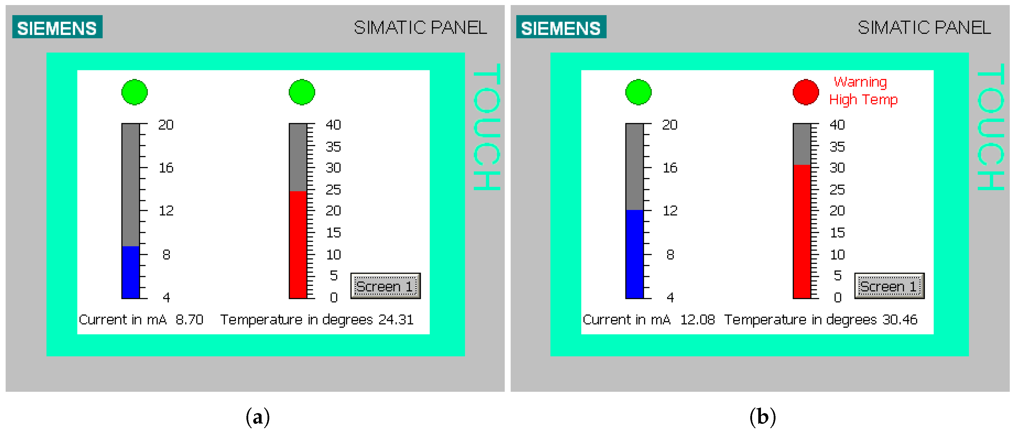
This was then used in the PLC software (Sematic Step7, Munich, Germany) to compute the temperature across a larger dynamic range. Although this may not be possible across the full range from 14–36 C due to the error bars, the dynamic range can be increased in this way as the PLC is capable of referring to a lookup table and interpolating results, so a linear response is not necessary. Both the current and the temperature were displayed in real time on bar graphs on the HMI, shown in Figure 11. Figure 11a shows an image of the HMI with the temperature in the normal operating range. Additionally, an alarm was programmed to be displayed when the temperature exceeded 30 degrees Celsius. This event is shown in Figure 11b.
5. General Discussion
5.1. Findings
This technique demonstrates that both digital and analogue signals from electrically-passive FOSs, with the aid of simple electronic circuitry, can be easily connected to corresponding digital and analogue input cards, on a standard industrial controller. In a commercial system, all of the electronics and electrical components could be embedded in a small optoelectronic box. Moreover, to take advantage of the benefits of FOSs, and to reduce the cost of the system, many digital and analogue sensors could be multiplexed together utilising a single optoelectronic unit.
The circuitry required to make an FBG compatible with a PLC system proved to be simple and easy to implement. The final circuit designs (Figure 4 and Figure 7), which made use of six operational amplifiers each, could be easily implemented in a single system-on-a-chip.
The usefulness of FBG sensors can be customized for a given application. Here, an arbitrary pressure switch and a temperature sensor were used as a simple proof of concept, although the method and results would be consistent with many other measurands. Moreover, by matching the laser to an FBG with different spectral characteristics [26], different response curves could be realized (Figure 10). The response could be made steeper to give a more defined switching signal, using an FBG with a square-like reflection spectrum. Alternatively, a more linear transfer function could be obtained for sensing purposes, by utilizing a broadband FBG with a linear edge, meaning the output current could be linear from 4 mA–20 mA and the temperature could span a much greater range, from 0 C–100 C, for example. The off-the-shelf bare FBG used in this example was used to demonstrate a proof of principle. For maximum dynamic range, long period gratings have a greater FWHM, although there is a trade-off between dynamic range and sensitivity as discussed in [27]. Moreover, the responsivity of standard FBGs to temperature can be customised to be as low as 7.49 pm C, increasing the dynamic range of their response as shown in [28]. Alternatively, FBGs encapsulated in different materials with different thermal properties could improve the range of the sensor as shown in [29]. Another consideration is the thermal stability of the FBG, as high temperatures can degrade the gratings [30].
The characteristics of the laser source can also play a significant part in the response of the sensors in this type of configuration. This has been explored in [31]. In general, the narrower the line width compared to the FWHM of the FBG, the higher the precision in the measurement, although there is usually a trade-off between the improved properties of the laser source and the cost of the laser.
Figure 6 and Figure 11 demonstrate an example of the kind of information that can be provided by the PLC and displayed using an HMI. Obviously, the complexity of the PLC program and the HMI will depend directly on the real application in which a system similar to this could be used; although by focusing only on the linear region of the output, no additional programming would be required to convert the current signal into the appropriate measurand.
This work is the first step in creating a PLC FOS interface by developing a digital input interface and a standard 4–20 mA analogue input interface. Put simply, we have replaced a traditional electrical/electronic instrument with an optical fibre equivalent, using industry standards. To the author’s knowledge, this has not been reported previously.
5.2. Significance
The main advantage of the approach detailed in this report is that the FOSs effectively become “plug and play” instruments with regard to current industrial controllers. All FBG interrogators on the market at present are expensive stand-alone systems that require knowledge of optical engineering. There has been some attempt to develop simpler, more compact FBG interrogators utilising smart controllers, such as field programmable gate arrays [32]. However, their penetration into mainstream industries has been extremely limited. By interfacing directly with standard industrial controllers, from an operational point of view, the control system is identical, with no need for additional training or programming.
6. Conclusions
In this work, we have demonstrated that both digital and analogue signals from FBG sensors can be integrated seamlessly into PLC-based control systems using a transmit-reflect detection system. The output from an in-ground FBG pressure switch was connected to existing PLC digital input using a simple conditioning circuit. The optoelectronic circuit took in the signals from two PIN photoreceivers, differentially amplified them and then used a comparator circuit to determine if the voltage resulted in a one or a zero at the digital input card, which was then used to trigger an alarm that was displayed on an HMI. This demonstrates that conventional “wired” switches can easily be replaced with optical switches without replacing the expensive PLC hardware. In addition, an arbitrary FBG sensor has been interfaced with a PLC using the 4–20-mA industry standard. The change in temperature, recorded by the FBG sensor, was displayed on the PLC’s HMI as a result of an optoelectronic conversion. The optoelectronic circuit again took in the signals from two PIN photoreceivers, differentially amplified them, added a DC offset and then converted the 1–5 V signal to the required 4–20 mA, using a transconductance amplifier. These relatively simple methods enable FOS to be utilised in established process control environments, combining state-of-the-art sensing with rugged industrial controllers. In addition, we have also outlined the development of an intelligent FOS network, utilizing standard PLCs for advanced industrial automation systems in the future, based on this work.
Author Contributions
All author’s contributed equally to the content of this article.
Conflicts of Interest
The authors declare no conflict of interest.
References
- Kouthon, T.; Decotignie, J.D. Improving time performances of distributed PLC applications. In Proceedings of the IEEE Emerging Technologies and Factory Automation, Kauai, HI, USA, 18–21 November 1996; Volume 2, pp. 656–662. [Google Scholar]
- Bolton, W. Programmable Logic Controllers, 5th ed.; Newnes: New South Wales, Australia, 2009. [Google Scholar]
- Belai, I.; Drahoš, P. The industrial communication systems Profibus and PROFInet. Appl. Nat. Sci. 2009, 329–336. Available online: http://citeseerx.ist.psu.edu/viewdoc/download?doi=10.1.1.468.7320&rep=rep1&type=pdf (accessed on 7 December 2017).
- Mitschke, S. Fieldbus Diagnostics: Latest Advancements Optimize Plant Asset Management; Technical Report; Fieldbus Foundation: Austin, TX, USA, 2007. [Google Scholar]
- Ozkul, T. Data Acquisition and Process Control Using Personal Computers; Marcel Dekker Inc.: New York, NY, USA, 1996. [Google Scholar]
- Chen, J.; Liu, B.; Zhang, H. Review of fibre Bragg grating sensor technology. Front. Optoelectron. China 2011, 4, 204–212. [Google Scholar] [CrossRef]
- Bunganaen, Y.; Lamb, D. An optical fibre technique for measuring optical absorption by chromophores in the presence of scattering particles. J. Phys. Conf. Ser. 2005, 15, 67. [Google Scholar] [CrossRef]
- Poeggel, S.; Tosi, D.; Duraibabu, D.; Leen, G.; McGrath, D.; Lewis, E. Optical fibre pressure sensors in medical applications. Sensors 2015, 15, 17115–17148. [Google Scholar] [CrossRef] [PubMed]
- Giallorenzi, T.G.; Bucaro, J.A.; Dandridge, A.; Sigel, G.H.; Cole, J.H.; Rashleigh, S.C.; Priest, R.G. Optical fibre sensor technology. IEEE J. Quantum Electron. 1982, 18, 626–655. [Google Scholar] [CrossRef]
- Zhong, D.; Tong, X. Application research on hydraulic coke cutting monitoring system based on optical fibre sensing technology. Photonic Sens. 2014, 4, 147. [Google Scholar] [CrossRef]
- Berthold, J.W.; Needham, D.B. Practical Application of Industrial Fiber Optic Sensing Systems; Instrument Society of America: Pittsburgh, PA, USA, 2006; Volume 61, p. 100. Available online: http://davidson-instruments.com/White_Papers_and_Standards/TAMU0106.pdf (accessed on 7 December 2017).
- Wild, G.; Hinckley, S. Distributed optical fibre smart sensors for structural health monitoring: A smart transducer interface module. In Proceedings of the 2009 5th IEEE International Conference on Intelligent Sensors, Sensor Networks and Information (ISSNIP), Melbourne, Australia, 7–10 December 2009; pp. 373–378. [Google Scholar]
- Morey, W.W.; Meltz, G.; Glenn, W.H. Fibre optic Bragg grating sensors. Proc. SPIE 1989, 1169, 98–107. [Google Scholar]
- Meltz, G.; Morey, W.W.; Glenn, W.H. Formation of Bragg gratings in optical fibres by a transverse holographic method. Opt. Lett. 1989, 14, 823–825. [Google Scholar] [CrossRef] [PubMed]
- Kersey, A. Multiplexed Bragg grating fibre sensors. In Proceedings of the IEEE Lasers and Electro-Optics Society Annual Meeting, Boston, MA, USA, 31 October–3 November 1994; Volume 2, pp. 153–154. [Google Scholar]
- Lee, B.; Jeong, Y. Interrogation Techniques for Fibre Grating Sensors and the Theory of Fibre Gratings. In Fiber Optic Sensors; Marcel Dekker: New York, NY, USA, 2002. [Google Scholar]
- Othonos, A.; Kalli, K. Fiber Bragg Grating Fundamentals and Applications in Telecommunications and Sensing; Artech House: Boston, MA, USA, 1999. [Google Scholar]
- Kashyap, R. Fiber Bragg Gratings; Academic Press: San Diego, CA, USA, 1999. [Google Scholar]
- Kersey, A.D.; Davis, M.A.; Patrick, H.J.; LeBlanc, M.; Koo, K.; Askins, C.; Putnam, M.; Friebele, E.J. Fiber grating sensors. J. Lightwave Technol. 1997, 15, 1442–1463. [Google Scholar] [CrossRef]
- Lopez-Amo, M.; Lopez-Higuera, J.M. Multiplexing Techniques for FBG Sensors in Fiber Bragg Grating Sensors: Research Advancements, Industrial Applications and Market Exploitation; A Cusano and A Cutolo; Bentham Science: Sharjah, UAE, 2014; pp. 99–115. [Google Scholar]
- Rao, Y.J. In-fibre Bragg grating sensors. Meas. Sci. Technol. 1997, 8, 355–375. [Google Scholar] [CrossRef]
- Nosenzo, G.; Whelan, B.; Brunton, M.; Kay, D.; Buys, H. Continuous monitoring of mining induced strain in a road pavement using fibre Bragg grating sensors. Photonic Sens. 2013, 3, 144–158. [Google Scholar] [CrossRef]
- Wild, G.; Hinckley, S.; Jansz, P. A transmit reflect detection system for fibre Bragg grating photonic sensors. Proc. SPIE 2008, 6801. [Google Scholar] [CrossRef]
- Allwood, G.; Wild, G.; Hinckley, S. Programmable Logic Controller Based Fibre Bragg Grating in-Ground Intrusion Detection System; Security Research Centre, Edith Cowan University: Perth, Australia, 2011; pp. 1–8. [Google Scholar]
- Bejan, C.; Iacob, M.; Andreescu, G. SCADA automation system laboratory, elements and applications. In Proceedings of the 7th IEEE International Symposium on Intelligent Systems and Informatics, Subotica, Serbia, 25–26 September 2009; pp. 181–186. [Google Scholar]
- Wen, K.; Yan, L.; Pan, W.; Luo, B. Design of fibre Bragg gratings with arbitrary reflective spectrum. Opt. Eng. 2011, 50, 54003. [Google Scholar] [CrossRef]
- James, S.W.; Tatam, R.P. Optical fibre long-period grating sensors: Characteristics and application. Meas. Sci. Technol. 2003, 14, R49. [Google Scholar] [CrossRef]
- Gwandu, B.A.L.; Zhang, W. Tailoring the temperature responsivity of fibre Bragg gratings [temperature/strain sensors]. In Proceedings of the IEEE Sensors 2004: 3rd IEEE International Conference on Sensors, Vienna, Austria, 24–27 October 2004; pp. 1430–1433. [Google Scholar]
- Mamidi, V.R.; Kamineni, S.; Ravinuthala, L.S.P.; Thumu, V.; Pachava, V.R. Characterization of encapsulating materials for fibre Bragg grating-based temperature sensors. Fiber Integr. Opt. 2014, 33, 325–335. [Google Scholar] [CrossRef]
- Zhang, B.; Kahrizi, M. High-temperature resistance fibre Bragg grating temperature sensor fabrication. IEEE Sens. J. 2007, 7, 586–591. [Google Scholar] [CrossRef]
- Wild, G.; Richardson, S. Analytical modeling of power detection-based interrogation methods for fibre Bragg grating sensors for system optimization. Opt. Eng. 2015, 54, 97109. [Google Scholar] [CrossRef]
- Kunzler, W.; Zhu, Z.; Selfridge, R.; Schultz, S.; Wirthlin, M. Integrating fibre Bragg grating sensors with sensor networks. In Proceedings of the IEEE 2008 AUTOTEST Conference: System Readiness Technology Conference, Salt Lake City, UT, USA, 8–11 September 2008; pp. 354–359. [Google Scholar]
Figure 1.
Principle of operation of an FBG optical switch. (a) The FBG and laser spectra are matched, resulting in maximum reflected intensity, and hence, the switch is in the off state; (b) The FBG and laser spectra are separated, resulting in minimum reflected intensity, and hence, the switch is in the on state.

Figure 2.
Principle of operation of transmit-reflect detection; (a) the reflected () and transmitted () intensities are approximately equal; (b) as the Bragg wavelength of the FBG increases, most of the intensity of the laser is transmitted, and a small portion is reflected; (c) as the Bragg wavelength of the FBG decreases, most of the intensity of the laser is reflected, and a small portion is transmitted.
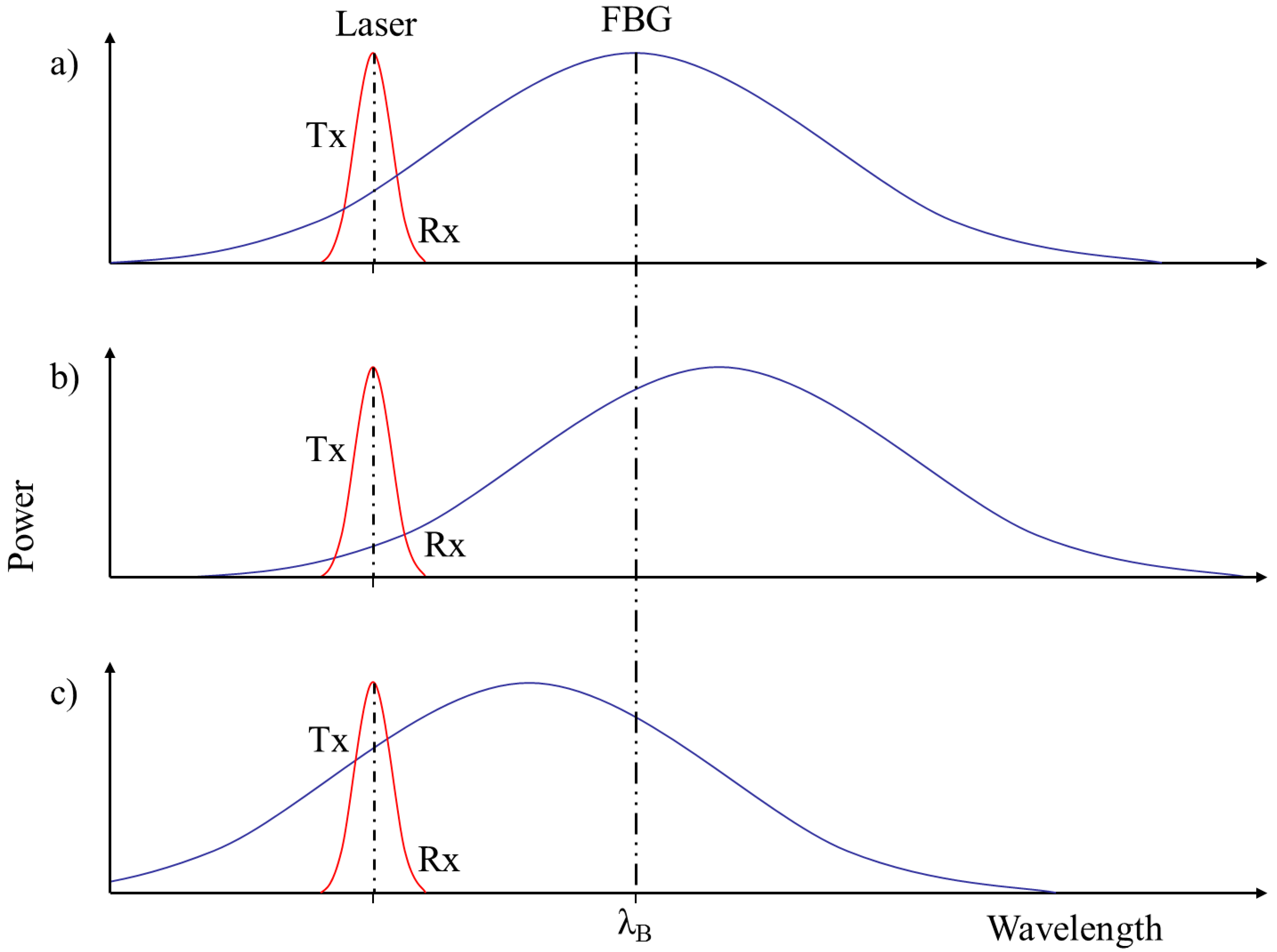
Figure 3.
Output from an optical fibre in-ground pressure switch showing an increase of approximately 0.5 V when stepped on.
Figure 3.
Output from an optical fibre in-ground pressure switch showing an increase of approximately 0.5 V when stepped on.

Figure 4.
Schematic of the PLC FOS digital input interface, including the receivers, differential amplifier and comparator circuit.
Figure 4.
Schematic of the PLC FOS digital input interface, including the receivers, differential amplifier and comparator circuit.

Figure 5.
Experimental setup for the digital input interface connected to the PLC I/O rack.
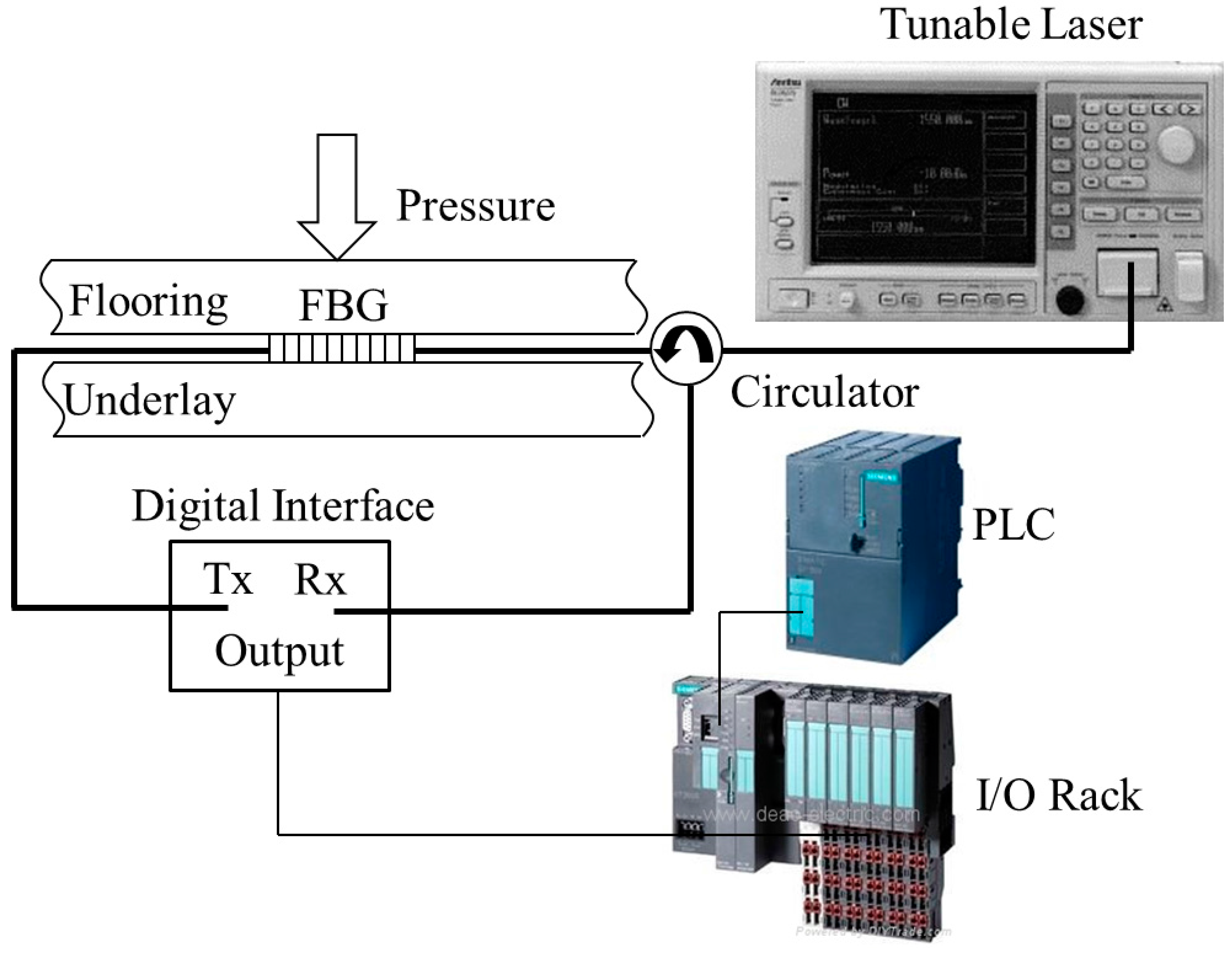
Figure 6.
A simple HMI display for (a) a secure perimeter and (b) a security breach.
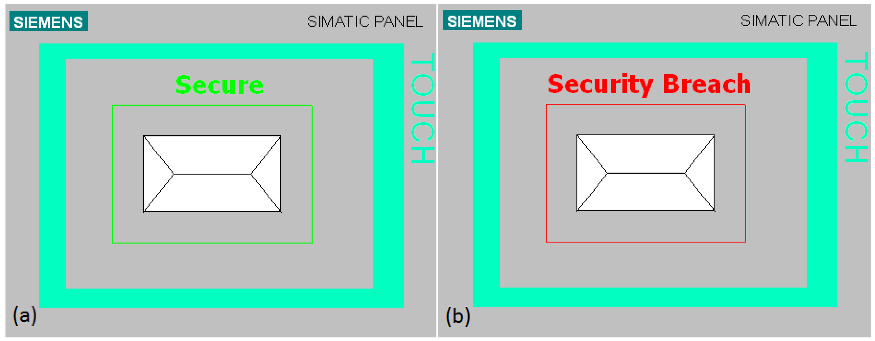
Figure 7.
Schematic of the PLC Fibre Optic Sensor (FOS) analogue input interface, including the receivers, differential amplifier and transconductance amplifier.
Figure 7.
Schematic of the PLC Fibre Optic Sensor (FOS) analogue input interface, including the receivers, differential amplifier and transconductance amplifier.
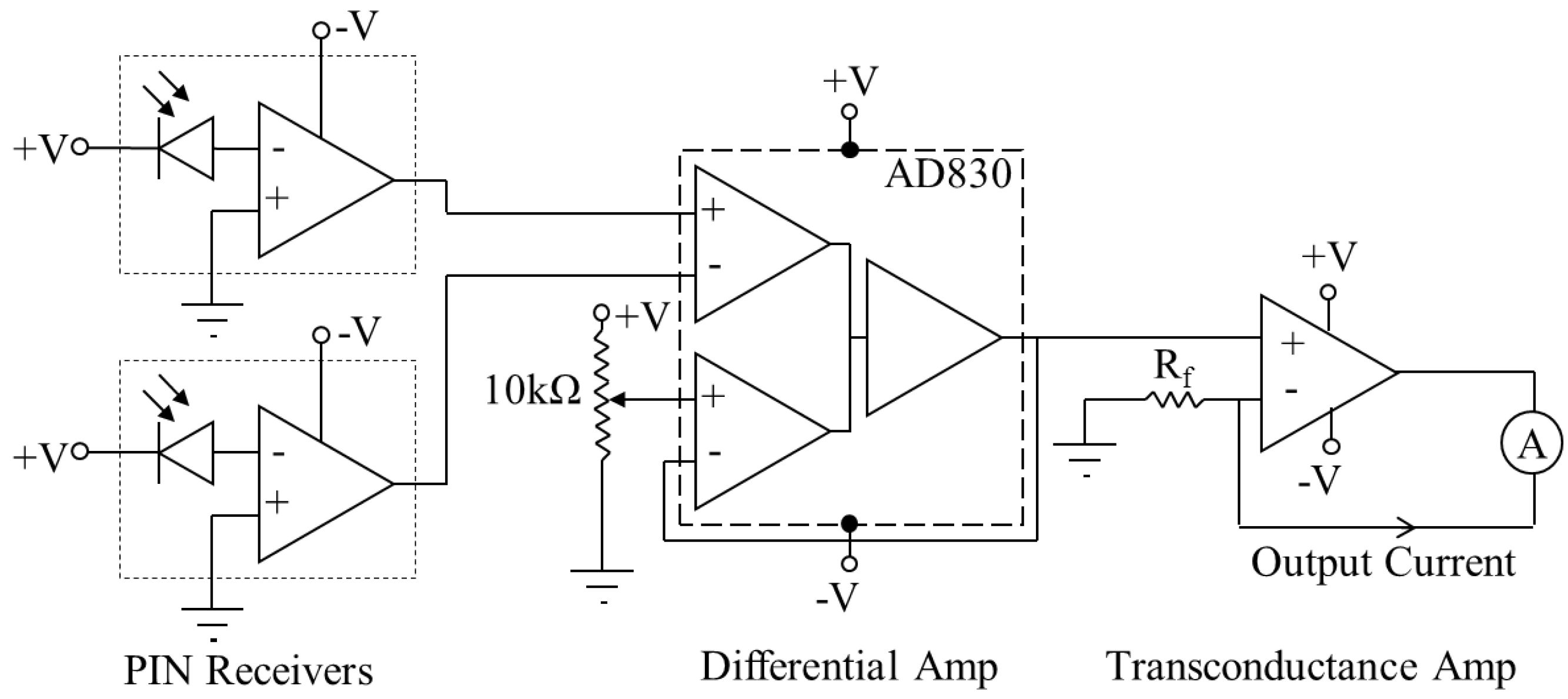
Figure 8.
The transfer function of the transconductance amplifier, showing the output current as a function of the measured input voltage difference.
Figure 8.
The transfer function of the transconductance amplifier, showing the output current as a function of the measured input voltage difference.

Figure 9.
Setup for the temperature characterisation experiment.
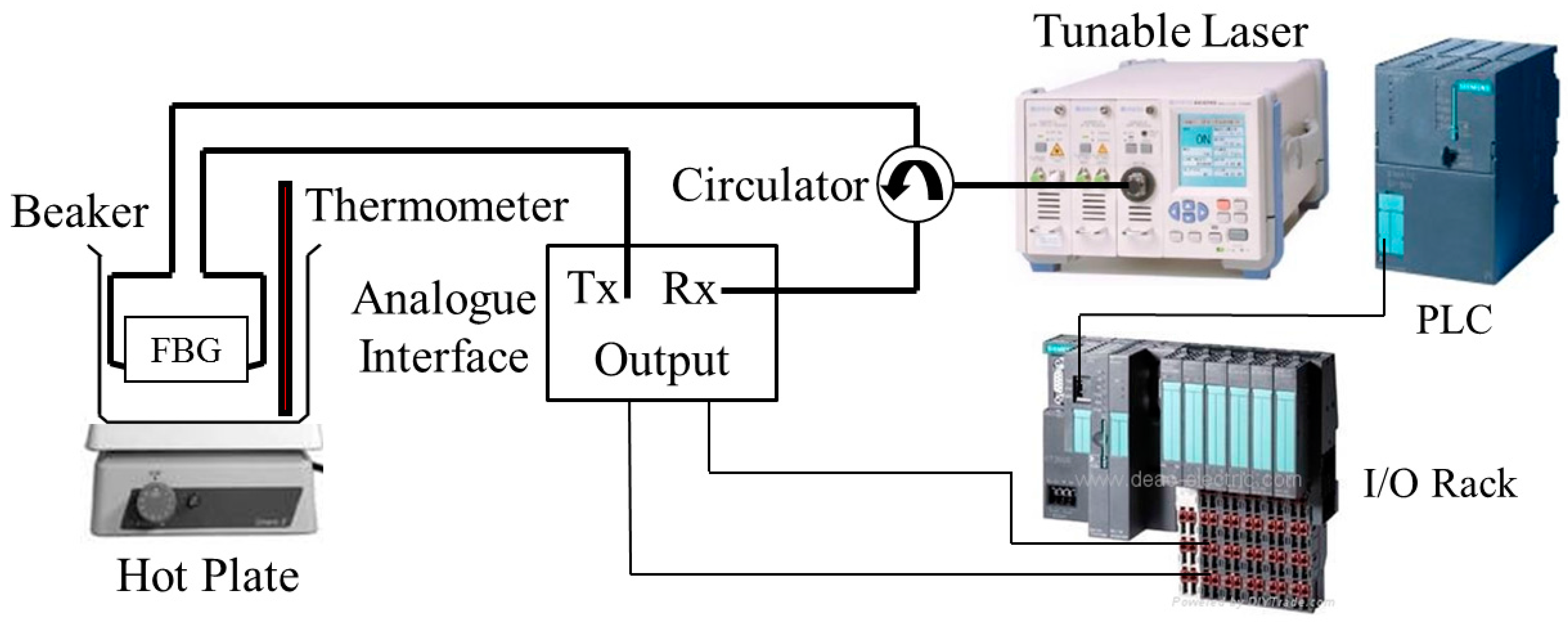
Figure 10.
Output current as a function of temperature.
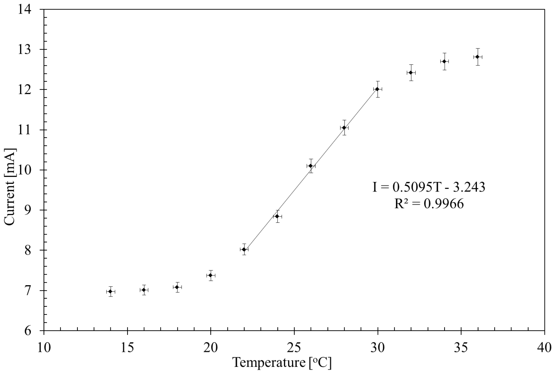
Figure 11.
Image of HMI panel created in WinCC Flexible. (a) Temperature below 30 degrees Celsius; (b) Temperature above 30 degrees Celsius with the high temperature alarm active.
Figure 11.
Image of HMI panel created in WinCC Flexible. (a) Temperature below 30 degrees Celsius; (b) Temperature above 30 degrees Celsius with the high temperature alarm active.

© 2017 by the authors. Licensee MDPI, Basel, Switzerland. This article is an open access article distributed under the terms and conditions of the Creative Commons Attribution (CC BY) license (http://creativecommons.org/licenses/by/4.0/).
Share and Cite
MDPI and ACS Style
Allwood, G.; Wild, G.; Hinckley, S. Universal Signal Conditioning Technique for Fiber Bragg Grating Sensors in PLC and SCADA Applications. Instruments 2017, 1, 7. https://doi.org/10.3390/instruments1010007
AMA Style
Allwood G, Wild G, Hinckley S. Universal Signal Conditioning Technique for Fiber Bragg Grating Sensors in PLC and SCADA Applications. Instruments. 2017; 1(1):7. https://doi.org/10.3390/instruments1010007
Chicago/Turabian StyleAllwood, Gary, Graham Wild, and Steven Hinckley. 2017. "Universal Signal Conditioning Technique for Fiber Bragg Grating Sensors in PLC and SCADA Applications" Instruments 1, no. 1: 7. https://doi.org/10.3390/instruments1010007