
Lane Detection via Object Positioning Systems Based on CCD Array Geometry

Institute of Vehicle Engineering, National Changhua University of Education, Changhua 500, Taiwan
Inventions 2016, 1(3), 16; https://doi.org/10.3390/inventions1030016
Submission received: 28 July 2016
/
Accepted: 18 August 2016
/
Published: 26 August 2016
(This article belongs to the Special Issue New Inventions in Vehicular Guidance and Control)
Abstract
:This paper presents an approach to lane detection for a vehicle. The positions of the lane marks can be evaluated by visual information of the image captured from a single charge-coupled device (CCD) camera. This proposed approach originally utilizes the properties of the CCD array in a camera to achieve the aim of objects positioning, since one pixel information produces two equations and increases one unknown variable. After camera calibration, this approach can therefore evaluate the intrinsic parameters of a camera from more pixel information. The configuration of the CCD chip cells is the key factor in this approach. The pixels of a resulting image directly reflect the geometry of the CCD cell, or the CCD array, in the camera. According to the attitude of the camera, this paper constructs the coordinate transformation that can resolve the geometrical relations between the film coordinate (the CCD array) and a fixed coordinate. This paper also provides associated techniques to facilitate the proposed approach, including image geometry analysis, distribution analysis of the CCD array, least mean square error (LMS) algorithm, etc. A down scaled experiment for lane detection is used to verify the feasibility of the proposed approach. The results show that the proposed approach is able to achieve object positioning.

1. Introduction
Over the past decades, considerable effort has been put towards the study of object position evaluation by computer visual information. Various approaches and techniques have been developed throughout manifold applications, including both applications and theories. Some used more than one camera so as to establish the position information of an object [1,2,3,4]. Rankin et al. addressed a stereo vision-based terrain mapping method for the off-road autonomous navigation of an unmanned ground vehicle (UGV) [1]. Chiang et al. developed a stereo vision 3D position measurement system for a three-axial pneumatic parallel mechanism robot arm [2]. Richa et al. presented an efficient approach for heart surgery by using stereo images from a calibrated stereo endoscope in medical application [3]. Luna et al. have studied a sensor system to measure the 2-D position of an object that intercepts a plane in space [5]. However, it may be laden to equip with two or more cameras in some applications. For instance, Zhou presented an approach to geo-locate the ground-based object from video stream by a single camera equipped in an unmanned aerial vehicle (UAV) [6]. The measuring system from the vision information may not be one of the main functions in some applications, but the system can provide more advantageous functions for those applications without implementing any extra hardware or device.
Camera calibration of is one of the crucial issues in computer vision. Camera parameters which require calibration include intrinsic and extrinsic ones [7]. The internal camera geometric and optical characteristics are intrinsic, while the 3D position and orientation of the camera frame relative to a certain world coordinate system are extrinsic. The intrinsic parameters of a camera are sometimes fixed, such as mounted orientation and position, distortion, CCD chip position, chip cell distance, etc. Although not all the techniques need any calibration object, the calibration of a camera is indispensable for some techniques of computer vision applications [8,9,10,11].
A sensor system which evaluates the positions of objects by visual information with a single CCD camera is presented. Some techniques of this proposed approach were adopted from the invention patented in Taiwan [12]. It utilizes the properties of the CCD array in a camera in order to measure the positions of objects that are on regular geometric lines, curves, or surfaces. This paper not only adopts the approach to solve the lane detection problems, but provides the evaluation procedure and discusses its errors. The technique in this study may not have to utilize any calibration object and can be regarded as self-calibration, or the so-called 0D approach [13]. The intrinsic parameters of the camera need to be obtained. This will result in a mathematical problem if all intrinsic parameters are evaluated by an image taken from the camera, although no calibration objects are necessary. An overview of this area can be found in [14] and the references therein. For example, the distortion calibration must be considered for most cameras. The distortion parameters—which are the intrinsic parameters of a camera—are constant for all pixels in an image taken by this camera [9]. This paper takes into account the radial distortion, since the radial distortion contributes the major errors to the distortions of the camera in this study. This paper details the mathematical model of the camera system in regard to the coordinate transformation between a fixed coordinate and a CCD chip coordinate. It also constructs the computational procedure for the object positioning system.
The notations in this paper are as follows: [.] denotes a matrix; denotes the position vector of point P, while denotes the origin position vector of A-coordinate; denotes the x, y, and z components of a position vector in A coordinate, that is,
where the unit vectors , , and are the orthogonal bases of A coordinate in x, y, and z axes, respectively. Hereafter in this paper, the position vector is in the fixed coordinate as the symbol A is omitted. It is intuitive that a vector can be represented both in A coordinate and B coordinate. That is,
or
2. Coordinate Transformation
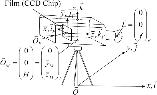
A spatial object can map on the corresponding chip cell of the CCD array, or the pixel in an image taken by a camera. From the pinhole phenomenon, the object—the mapped pixel on the CCD array—and the lens center should be collinear after calibration for the camera distortion. The mapped pixel on the CCD array and the lens center can formulate the line equation in algebra intuitively, and the other one can satisfy the line equation as long as their position vectors are represented in the same coordinate system. In general, we can use the fixed coordinate to represent these position vectors. Therefore, the coordinate transformation from the CCD array coordinate (or the film chip coordinate) to the fixed coordinate is significant by this approach. Figure 1 shows the relations between the fixed coordinate and the film chip coordinate, where and are the origins of the fixed coordinate and the film chip (CCD array) coordinate, respectively. For convenience, as shown in Figure 1, we can assign the orientations of the -axis and the -axis in the film chip coordinate to conform to the pixel orientations of the x-axis and y-axis in an image. Let and denote any position represented in the fixed coordinate and in the film chip coordinate, respectively; i.e.,
According to the definitions,
and
then,
In general, and . That is, the positions of objects can refer to the position of the camera. can also be represented in fixed coordinate; i.e., . In Figure 1, the mounted position for the camera, , where and can be obtained from the specifications of the camera. can be assigned just above the origin of the fixed coordinate with zero x-axis and zero y-axis components. has only the z component in the fixed coordinate, or , where H is the height of and H can be measured directly. According to (7),
The origin of the film chip coordinate represented in the fixed coordinate can be
where
and , , and denote the Euler angles of the camera for the yaw, pitch, and roll angles, respectively. Consequently, the coordinate transformation from the film chip coordinate to the fixed coordinate defined in (4) can become
In Figure 1, let be the lens center position where
Substituting (13) into (12), the lens center position in the fixed coordinate becomes
The CCD array, or the film chip of a camera, consists of the CCD cells which sense the light energy to make an image collected by the corresponding pixels. Figure 2 sketches the configuration of the CCD array, where U is the width of the CCD array, V is the height of the CCD array, is the width of the CCD cell, is the height of the CCD cell, and and are the numbers of the CCD cells on the film chip in the width and height directions, respectively. Let in which and denote the index of the CCD cells on the chip. is indeed the same as the pixel index of the image. Let stand for the position vector at the center of the chip cell for a pixel indexed by and in the image. Then, the chip cell center position can be as follows.
Substituting (15) into (12), the position at the center of the chip cell in the fixed coordinate in terms of the pixel index of the image becomes
This section has derived the positions of some significant points represented in the fixed coordinate from the film chip coordinate by the appropriate coordinate transformation in (12). According to (16), it can be intuitive to obtain the chip cell center position indexed by , which is also the pixel index of the image. Based on the pinhole model of a camera, an object from the scene mapped onto the CCD array, or the image, can be formulated as a line equation that makes two equations in three-dimensional (3D) space. In addition, the object in the scene, the lens center, and the center position vector of the corresponding chip cell mapped from the object must be collinear. If there are n objects, there should be n lines, or 2n equations. In the case that a set of the evaluated objects is on a regular curve (e.g., a line, a circle, etc.), n objects will increase n + 2 unknowns, including two regular curve parameters. Theoretically, the position evaluations for the objects are feasible since the equations increased are more than the unknowns increased. The Euler angles of the camera are not intrinsic parameters. They are sometimes fixed for images taken by the same camera in applications. However, the Euler angles will make the position evaluations inaccurate for a slight misalignment of the attitude for a camera.
3. The Evaluations of Camera Parameters and Object Positions
To exemplify the proposed approach, this paper assumes a case wherein the evaluated objects in the scene are collinear on the ground. According to the pinhole phenomenon, a point of the objects which are collinear with the equation on the ground (z = 0) maps on the CCD chip cell at a pixel indexed by . Therefore, points collinear on satisfy the line equation as follows.
or
where , , , , , and are defined in (14) and (15). If a set of points in a fixed coordinate maps onto a set of pixels in the image, or the CCD array, where , there will be 2n equations according to (18) and (19). In this evaluation approach, , , , and H are the fixed variables for an image, while the line parameters m and are also fixed, but only is a variable. One pixel information in an image produces two equations and one variable. Therefore, as for the objects on a regular curve, there should be at least pixel information in an image to solve the additional variables and fixed variables theoretically. In Figure 1, , , and the CCD geometry are known. If there is more than pixel information, the evaluations of camera parameters and positions of objects can apply the least square approach from the quadratic performance index. That is, if there are () pixel information on the j-th line (i.e., and are both constants for any j = 1, 2, ..., , where denotes the number of regular lines), the least square approach can be defined as , where J is the quadratic performance index and
The optimal evaluated values of the unknown variables, including fixed and additional ones, can be obtained if J is minimized. The solution of minimization in (20) might not converge to a unique one by numerical methods or mathematical algorithms. The solution highly depends on the initial guess values of the variables. There are two ways to improve the solution accuracy of (20) in calculations. One is to increase the number of objects on the same line. The other is to choose more accurate initial guess values of the variables.
Figure 3 shows an evaluation system with a DH-HV2003UC camera, while this paper uses the 3DM-GX1 gyro mounted on the camera in order to measure the exact attitude, or the Euler angles, of the camera. Regarding the verification purpose of this proposed approach, this paper compares the exact attitudes with the evaluated ones. It additionally utilizes a laser distance meter to measure the height more precisely from the ground (platform) to the mounted position of the camera on its stand. According to the specifications of this camera, the CCD chip parameters are as follows. , , , , , , , and . These parameters are crucial to the evaluation of the positions of objects by the proposed approach, since they play the key role in the accuracy of the position evaluation approach. As for the camera distortion calibrations, this paper only takes into account the radial distortion of the camera, rather than other types of distortions in this application, such as the decentering distortion, the thin prism distortion, etc. Based on the images taken by the camera, the radial distortion of this camera is of the barrel type, with a negative distortion constant equal to −8.3042 × 10⁻⁷ in pixels.
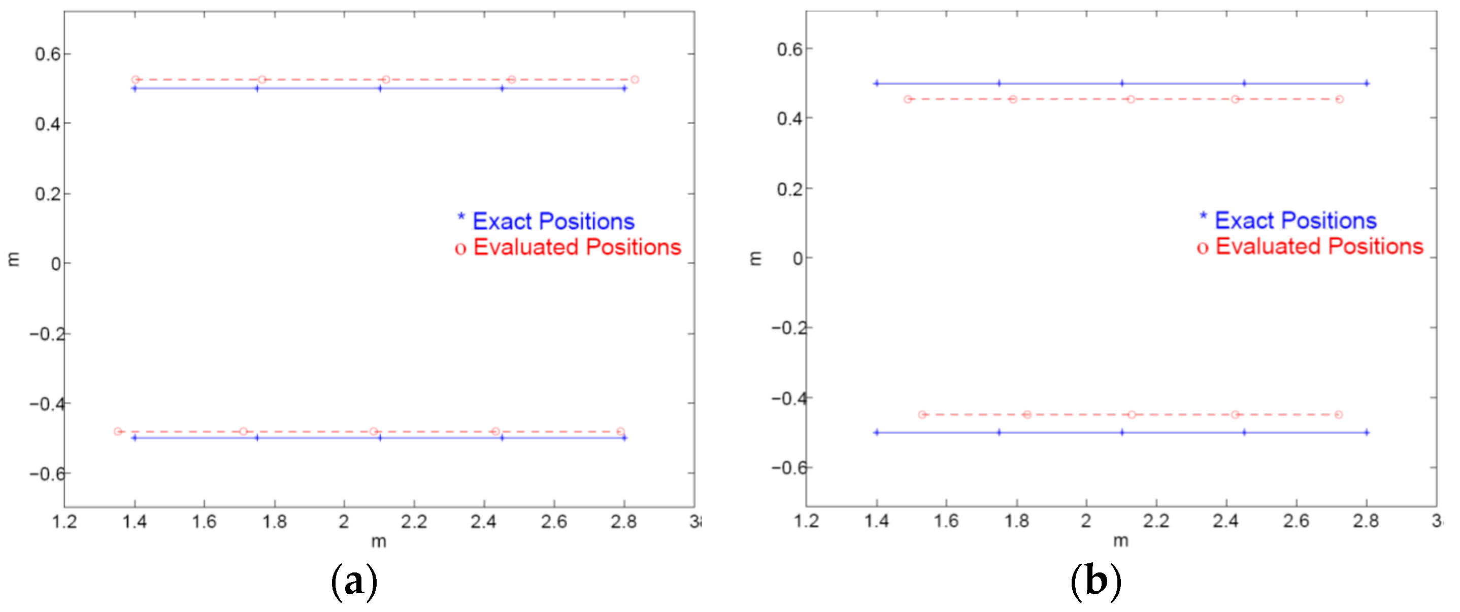
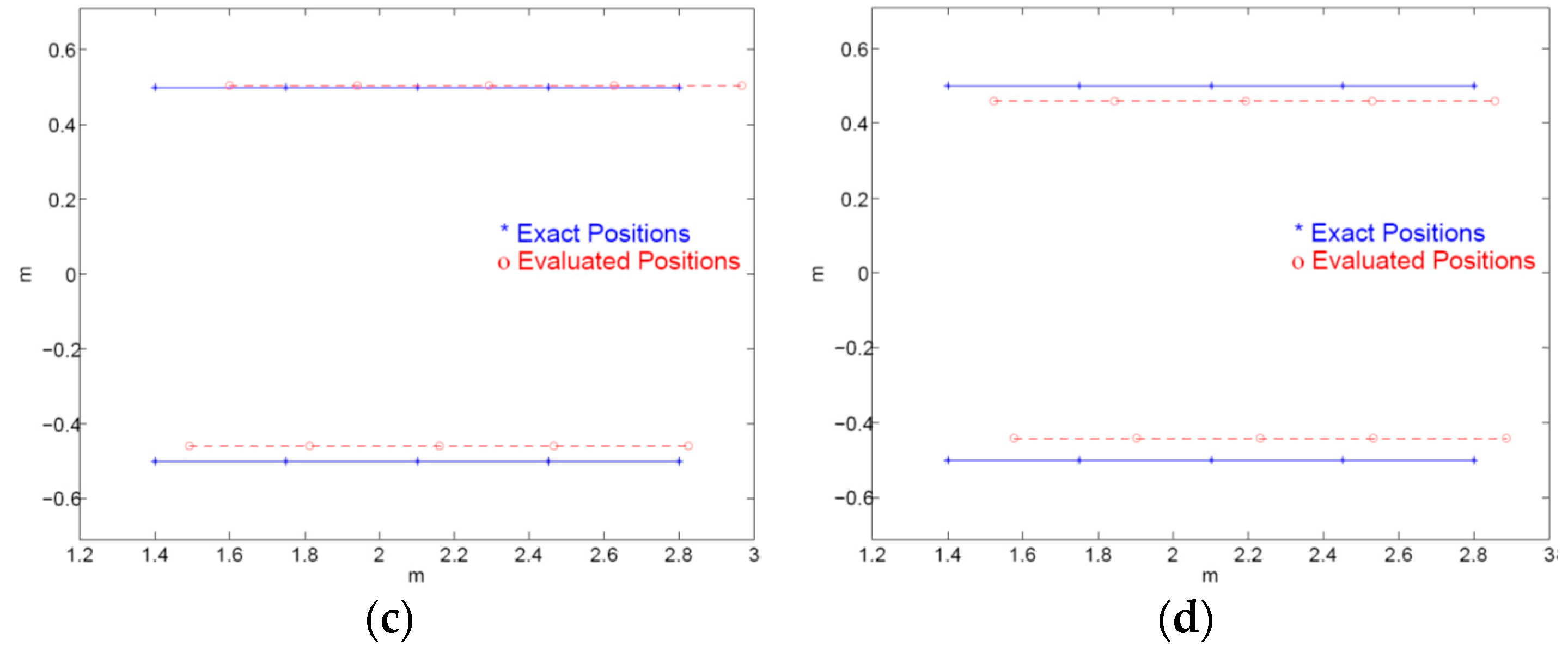
The position evaluation of the lane marks is a practical example, for instance, of the lane departure warning system of vehicles [15,16,17]. Figure 4 shows the downscaled simulation scenario for the position evaluation of the lane marks, while the geometry of the platform is also illustrated in Figure 4b. In this example, . There are four cases used to verify the feasibility of the proposed approach. They are the conditions as follows: (a) , , ; (b) , , ; (c) , , ; (d) , , , respectively. The nonzero Euler angles simulate the situations in which the position evaluations of the landmarks are on the road if there are misalignments for the attitudes of the camera equipped in a vehicle. Figure 5 shows the pictures taken by the camera for these four different cases. We can pick out the specified points as in Figure 4b with their corresponding pixel indices in the pictures after some adequate image processes. Table 1 lists the values of the corresponding pixel index, or and values, of the assigned lane marks in these four different pictures. The axes defined in the pixel coordinate conform to those defined in images. For instance, the definitions of y-axes in these different coordinates coincide with each other but in opposite directions in real space, because of the pinhole effect. Therefore, the directions of the x-axis and y-axis are, respectively, rightward and downward in pictures conventionally, but rightward and upward in film coordinate with front view. Figure 6 sketches the position evaluation results of the simulations in the case studies. The solid lines and the dashed lines stand for the exact positions and the evaluated positions of the assigned lane marks, respectively. The evaluated positions of those marks are all in the arithmetic progressions, and can be solved by numerical methods recursively. These results show that the proposed approach can evaluate the positions of specified collinear objects, even though there is a slight misalignment of the attitude for the camera. However, there are still errors between the exact positions and the evaluated ones. The errors may come from the accuracy of the camera geometry, the aspherical lens of camera, the accuracy of the pixel indexes chosen in the result pictures, etc.
The accuracy of the position evaluations depends on the mapped-on positions of the pixels of objects. The vehicle vibrations from rough roads, and the external image disturbances from ill environment such as rain, light, shadow, etc., are indeed the key factors which affect the recognition accuracy. In practice, the effects of vehicle vibrations are relatively small because of the shock absorbers on the vehicle. A camera stabilizer could be equipped for the sake of capturing a high quality image if the vehicle vibrations are tremendous. The effects of the image disturbances from the environment are one of the most significant issues. Some image process may overcome the image noise and disturbance problems such as medium filter, vector median filter, vector directional filter, adaptive median filter, adaptive nearest neighbor filter, etc.
4. Conclusions
This paper presents an approach to evaluate the positions of objects by utilizing a single camera. An image can provide the information of the objects captured on the CCD chip cells. For instance, a pixel can produce two equations and an additional variable. Besides, some variables for the camera are fixed. If the objects are in regular geometry, a limited amount of pixel information can form enough equations to solve the position evaluation problems via the coordinate transformation. The properties of the CCD array serve as the main reference dimensions for the evaluation of the positions of objects in an image. The accuracy of the position evaluations depends on the pixels of objects picked out in an image, while it is sometimes not easy to discern the exact pixels of objects in the image. That is, if the image position of a point is not exact, the results which depend on its image coordinate will cause erroneousness in the position evaluations of objects. The image disturbances from vehicle vibrations or image background are also significant for the position evaluation accuracy. It is suggested to equip a camera stabilizer if the vibrations are serious, and to apply some image filter to reduce the effect of image disturbances before the position evaluation. The initial guess of the evaluated variables in (20) is crucial, and will affect the approached solutions. Future study can focus on the number of pixels selected in an image that can abate the effects of the initial guess in the position evaluations of objects.
Acknowledgments
This research work is sponsored by Ministry of Science and Technology under Grand NSC 100-2221-E-018-017 and MOST 103-2221-E-018-23.
Author Contributions
The author contributes full of this work.
Conflicts of Interest
The author declares no conflict of interest.
References
- Rankin, A.L.; Huertas, A.; Matthies, L.H. Stereo vision based terrain mapping for off-road autonomous navigation. In Proceedings of the SPIE 7332, Unmanned Systems Technology XI, Orlando, FL, USA, 30 April 2009; pp. 733210–733217. [CrossRef]
- Chiang, M.-H.; Lin, H.-T.; Hou, C.-L. Development of a stereo vision measurement system for a 3D three-axial pneumatic parallel mechanism robot arm. Sensors 2011, 11, 2257–2281. [Google Scholar] [CrossRef] [PubMed]
- Richa, R.; Poignet, P.; Liu, C. Three-dimensional motion tracking for beating heart surgery using a thin-plate spline deformable model. Int. J. Robot. Res. 2010, 29, 218–230. [Google Scholar] [CrossRef]
- Dornaika, F.; Chung, C.R. Stereo geometry from 3-d ego-motion streams. IEEE Trans. Syst. Man Cybern. 2003, 33, 308–323. [Google Scholar] [CrossRef] [PubMed]
- Luna, C.A.; Lázaro, J.L.; Mazo, M.; Cano, A. Sensor for high speed, high precision measurement of 2-D positions. Sensors 2009, 9, 8810–8823. [Google Scholar] [CrossRef] [PubMed]
- Zhou, G. Geo-referencing of video flow from small low-cost civilian uav. IEEE Trans. Autom. Sci. Eng. 2010, 7, 156–166. [Google Scholar] [CrossRef]
- Tsai, R.Y. A versatile camera calibration technique for high-accuracy 3D machine vision metrology using off-the-shelf TV cameras and lenses. IEEE J. Robot. Autom. 1987, 3, 323–343. [Google Scholar] [CrossRef]
- Zhang, Z. A flexible new technique for camera calibration. IEEE Trans. Pattern Anal. Mach. Intell. 2000, 22, 1330–1334. [Google Scholar] [CrossRef]
- Weng, J.; Cohen, P.; Herniou, M. Camera calibration with distortion models and accuracy evaluation. IEEE Trans. Pattern Anal. Mach. Intell. 1992, 14, 965–980. [Google Scholar] [CrossRef]
- Maybank, S.J.; Faugeras, O.D. A theory of self-calibration of a moving camera. Int. J. Comput. Vis. 1992, 8, 123–152. [Google Scholar] [CrossRef]
- Gibbins, D.; Roberts, P.; Swierkowski, L. A Video Geo-Location and Image Enhancement Tool for Small Unmanned Air Vehicles (Uavs). In Proceedings of the 2004 Intelligent Sensors, Sensor Networks and Information Processing Conference, Melbourne, Australia, 14–17 December 2004; pp. 469–473.
- Young, J.-S. Object positioning determinated by the characteristic of image capturing devices and numerical methodology. I424373, 21 January 2014. [Google Scholar]
- Zhang, Z. Camera calibration with one-dimensional objects. IEEE Trans. Pattern Anal. Mach. Intell. 2004, 26, 161–174. [Google Scholar] [CrossRef] [PubMed]
- Heyden, A.; Pollefeys, M. Multiple view geometry. In Emerging Topics in Computer Vision; Medioni, G., Kang, S.B., Eds.; Prentice Hall: Upper Saddle River, NJ, USA, 2003; pp. 45–108. [Google Scholar]
- Wang, Y.; Teoh, E.K.; Shen, D. Lane detection and tracking using B-snake. Image Vis. Comput. 2004, 22, 269–280. [Google Scholar] [CrossRef]
- Nedevschi, S.; Schmidt, R.; Graf, T.; Danescu, R.; Frentiu, D.; Marita, T.; Oniga, F.; Poco1, C. 3D lane detection system based on stereovision. In Proceedings of the IEEE Intelligent Transportation Systems Conference, Washington, DC, USA, 3–6 October 2004.
- Jung, C.R.; Kelber, C.R. A lane departure warning system based on a linear-parabolic lane model. In Proceedings of the 2004 IEEE Intelligent Vehicles Symposium Conference, Sao Leopoldo, Brazil, 14–17 June 2004; pp. 891–895.
Figure 1.
Definitions of the fixed coordinate and the film chip coordinate.
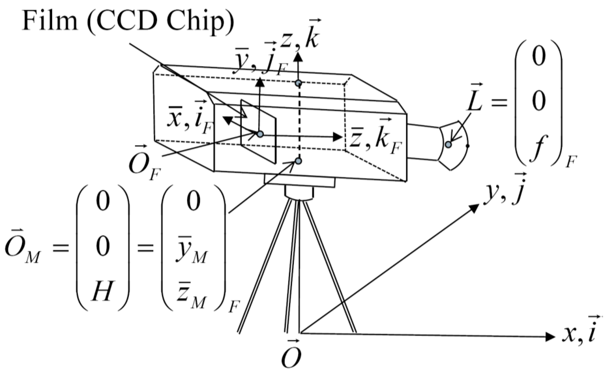
Figure 2.
The configuration of the chip cells for the film chip (CCD chip) in front view.
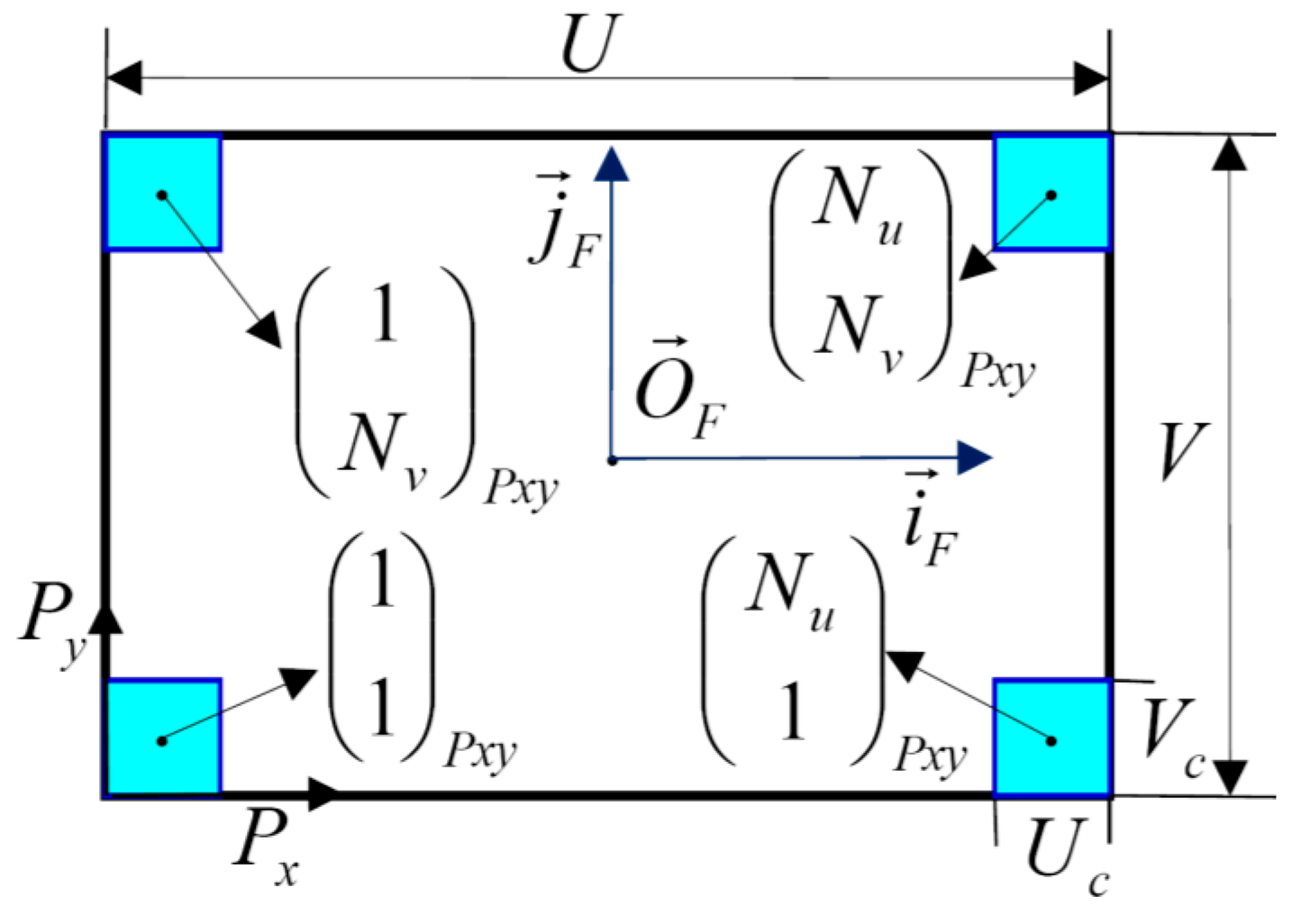
Figure 3.
The verification of the evaluation for the measurement system with gyroscope.
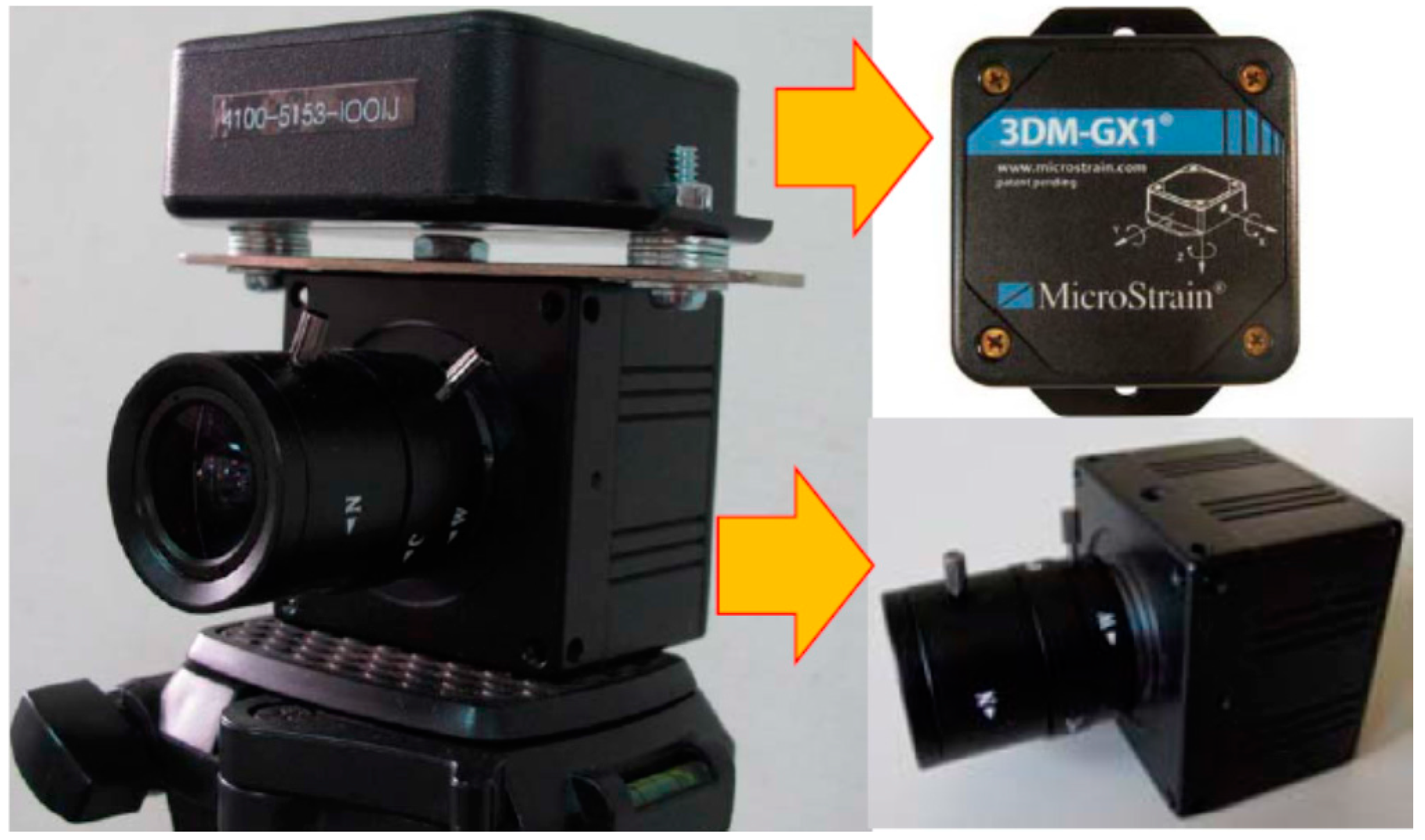
Figure 4.
The downscaled simulations for the position evaluation of the lane marks. (a) The scenario platform; (b) the geometry of the assigned 10 lane marks with alphabets on the scenario platform.
Figure 4.
The downscaled simulations for the position evaluation of the lane marks. (a) The scenario platform; (b) the geometry of the assigned 10 lane marks with alphabets on the scenario platform.

Figure 5.
The result pictures of the 4 scenarios as (a) , , ; (b) , , ; (c) , , ; (d) , , .
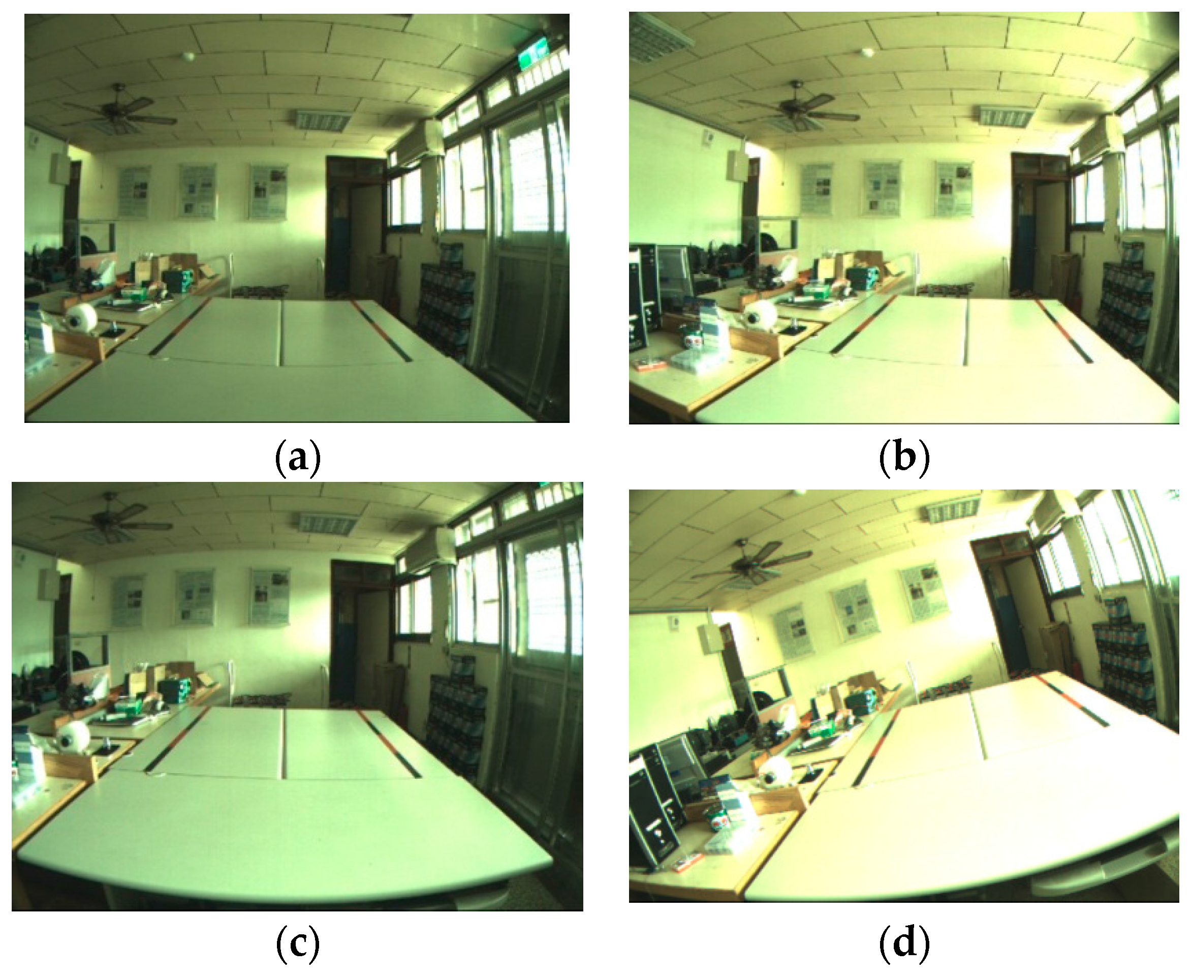
Figure 6.
The evaluation results of the 4 scenarios as (a) , , ; (b) , , ; (c) , , ; (d) , , .

| Mark | A | B | C | D | E | F | G | H | I | J | |
|---|---|---|---|---|---|---|---|---|---|---|---|
| (a) | 191 | 223 | 246 | 263 | 276 | 571 | 539 | 514 | 497 | 484 | |
| 501 | 470 | 448 | 430 | 416 | 509 | 476 | 452 | 434 | 419 | ||
| (b) | 301 | 334 | 360 | 377 | 389 | 666 | 638 | 618 | 602 | 590 | |
| 495 | 465 | 441 | 425 | 411 | 511 | 475 | 450 | 432 | 418 | ||
| (c) | 194 | 227 | 249 | 266 | 279 | 565 | 534 | 511 | 496 | 481 | |
| 403 | 370 | 344 | 327 | 313 | 413 | 378 | 351 | 333 | 318 | ||
| (d) | 334 | 356 | 374 | 385 | 394 | 691 | 653 | 626 | 606 | 590 | |
| 427 | 387 | 356 | 334 | 317 | 344 | 316 | 296 | 283 | 269 | ||
© 2016 by the author; licensee MDPI, Basel, Switzerland. This article is an open access article distributed under the terms and conditions of the Creative Commons Attribution (CC-BY) license (http://creativecommons.org/licenses/by/4.0/).
Share and Cite
MDPI and ACS Style
Young, J.-S. Lane Detection via Object Positioning Systems Based on CCD Array Geometry. Inventions 2016, 1, 16. https://doi.org/10.3390/inventions1030016
AMA Style
Young J-S. Lane Detection via Object Positioning Systems Based on CCD Array Geometry. Inventions. 2016; 1(3):16. https://doi.org/10.3390/inventions1030016
Chicago/Turabian StyleYoung, Jieh-Shian. 2016. "Lane Detection via Object Positioning Systems Based on CCD Array Geometry" Inventions 1, no. 3: 16. https://doi.org/10.3390/inventions1030016