Control of the Acrobot with Motors of Atypical Size Using Artificial Intelligence Techniques


Department of Artificial Intelligence, Faculty of Computer Science, Universidad Politécnica de Madrid, 28660 Madrid, Spain
*
Authors to whom correspondence should be addressed.
Inventions 2017, 2(3), 16; https://doi.org/10.3390/inventions2030016
Submission received: 1 July 2017
/
Revised: 29 July 2017
/
Accepted: 9 August 2017
/
Published: 14 August 2017
(This article belongs to the Special Issue Advances in Mechanism Design for Robots)
Abstract
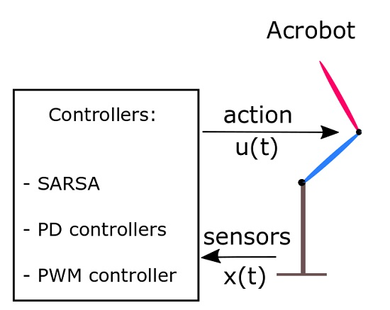
:An acrobot is a planar robot with a passive actuator in its first joint. The main purpose of this system is to make it rise from the rest position to the inverted pendulum position. This control problem can be divided in the swing-up issue, when the robot has to rise itself by swinging up as a human acrobat does, and the balancing issue, when the robot has to maintain itself in the inverted pendulum position. We have developed three controllers for the swing-up problem applied to two types of motors: small and large. For small motors, we used the State-Action-Reward-State-Action (SARSA) controller and the proportional–derivative (PD) controller with a trajectory generator. For large motors, we propose a new controller to control the acrobot—a pulse-width modulation (PWM) controller. All controllers except SARSA are tuned using a genetic algorithm.

1. Introduction
A planar robot is a robotic arm that moves on a plane. If a robot has less actuators than degrees of freedom, the system is called underactuated. An underactuated planar robot with two rotational joints could be a pendubot [1] if the passive actuator is the second joint , or an acrobot [2,3,4,5,6,7,8,9,10,11,12,13,14] if the passive actuator is the first joint (Figure 1).
The acrobot control problem is to make it rise from the rest position to the inverted pendulum position. As the first and second link of an acrobot are coupled, the control problem is split in two [3,4,6,7,8,9,12]: the swing-up problem, in which the acrobot has to rise itself above one meter as a human acrobat does; the balancing problem, in which it has to maintain itself in the inverted pendulum position. Other researchers have solved the whole problem with only one controller [5,10,13].
For the swing-up problem, Duong [4] proposed to use a NeuroController, Spong [9] and Brown [3] designed a proportional–derivative (PD) controller with a trajectory generator, and Mahindrakar [7] used an energy-based controller. Ueda [12] proposed a decision-making algorithm with several limitations of memory to solve the swing-up issue on acrobots with the capabilities available in a small robot. However, Sutton [10] solved the problem using reinforcement learning. He proposed State-Action-Reward-State-Action (SARSA)—an algorithm that learns by a trial and error method. SARSA uses a table () to save the states s that the acrobot visited, the actions a that took on that state, and the performance of taking that action on that state. Nichols [8] compared three other methods of reinforcement learning to solve the swing-up issue: Continuous Actor Critic Learning Automaton (CACLA), NerlderMead-SARSA (NM-SARSA) and NerlderMead-SARSA. He claims that NerlderMead-SARSA is faster than many other controllers in the literature.
The solutions proposed for the balancing problems use a linear–quadratic regulator (LQR) controller [3,4,7,9] or a fuzzy controller [3]. Duong, Brown, Mahindrakar, and Spong [3,4,7,9] tuned the parameters of the controllers using a genetic algorithm.
The acrobot problem was solved by Duong [5], as an extension of his previous work [4] with a NeuroController, and by Zhang [15] which used a spiking neural network with an LQR. Both used a genetic algorithm to improve the performance of their algorithms. Horibe [6] also solved the acrobot problem by a feedback law that was obtained by numerically solving a Hamilton–Jacobi equation by the stable manifold method.
Those papers proposed different methods to solve the acrobot problem, avoiding the saturation of the motors. The controllers made by Sutton [10] (SARSA) and Spong [9] (PD controller) can work with motors with low maximum torque, but none of them tried to take advantage of the saturation of motors with high maximum torque.
In this paper, we propose two variants of the SARSA algorithm [10]: to initialize the algorithm with zeros or non-zero values and to introduce some error on the sensors of the acrobot. As the PD controller proposed by Spong [9] is not a traditional PD controller, we have also compared his PD controller with a canonical PD controller. Finally, we propose a novel pulse-width modulation (PWM) controller that uses the saturation of a large motor to control the acrobot in any operation point of the first joint.
2. Acrobot Model
All the controllers were tested on a simulated acrobot. The parameters of our acrobot are shown in Table 1.
The equations of motion of the system are the same as those of a planar robot without the input torque on the first joint:
where is the inertia matrix, is the acceleration of Coriolis, the gravitation terms, and are the accelerations (rad/s2) of the first and second joint, and are the velocities (rad/s) of the first and second joint, and are the position (rad) of the first and second joint, and is the input torque on the second joint. The other terms on the Equation (1) are shown in the Equations (2).
The control time used for all the controllers is ms. The calculus of and is performed four times between one control input and the next one. The positions of the first and second joint (,) are between , the velocity of the first joint () is between , and the velocity of the second joint () between .
To control an acrobot with these parameters, a motor with a maximum torque of Nm can be used. We used smaller motors for the SARSA and the PD controller ( Nm), and larger for the PWM controller ( Nm). The sensors are simulated, with an added error of of the range of each dimension (only used for the SARSA controller). The sensors are thus able to read the position and the velocities of the first and the second joint, but not the accelerations.
3. Control Methods
3.1. State-Action-Reward-State-Action (SARSA) Controller
SARSA [10] is a reinforcement learning algorithm that can learn through experience (on-line learning), which can take the best action at each moment to achieve its goal. Generally, it uses a table that associates states and actions, which stores the weights of how good an action a is at a state s. The SARSA algorithm is shown in Algorithm 1.
To create , it is necessary to discretize the range of each dimension in parts, in order to make the infinite range of the values a finite range of possible states. The combination of the discretized dimensions is called “tiling”. It is possible to use more than one tiling, changing the updating rule for:
Sutton [10] used 48 tiles (12 with 4 dimensions, 12 with 3 dimensions, 12 with 2 dimensions, and 12 with 1 dimension). The position and the velocity range are split in six intervals, but the dimensions of the velocities are offset by a random fraction of interval, so they have seven intervals.
| Algorithm 1: SARSA algorithm |
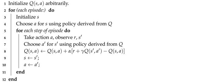 |
As we have used a small motor with a maximum torque of Nm, the only possible actions are . The reward r used is until the end of the acrobot is above 1 m. For the election of the action a, a greedy policy (with ) is used, because a bad move could end a set of good moves. A learning rate () is equal to because a low value () saves the old information learned while the system continues learning, and it is divided by 48 because we use 48 tiles. The discount factor is high ( = 1) to search for long-term reward.
In Section 4.1, we have compared the results (Figure 2) obtained when are initialized with zero (Figure 2a,b) or non-zero (Figure 2c,d) values, as two possible ways to initialize arbitrarily, and when an error of of the range on , , , and (Figure 2b,d) are introduced to the sensors.
3.2. Proportional–Derivative (PD) Controller
Spong [9] proposed a PD controller to solve the swing-up problem:
where and are the proportional and derivative terms of the PD controller, and the terms , y are:
This equation is not exactly a PD controller. The canonical controller used is:
If the torque compensation is taken apart:
However, a PD controller uses the following formula:
where . When these two formulas are equated to compare if there are differences:
We obtain that the last Equation (18) is not always true. In Equation (4), the desired velocity (right part of (18)) of the second joint has a constant value (=0); meanwhile, the classic PD controller computes that value as the derivate of the error (left part of (18)).
The controller is tuned by a genetic algorithm. The fitness is the needed time of the acrobot to go above 1 m.
where is the position on the y axis of the end of the acrobot, h is the threshold of one meter to achieve the goal of the swing-up problem, and t is the time when the acrobot go above the threshold. If the acrobot controller cannot solve the swing-up problem, the fitness is very high.
The best third part of each population (those which have less fitness) is maintained for the next generation (33% of elitism). A linear ranking selection (Equation (20)) is a selection operator that selects the parents of the reproduction operator using a probability that depends on their rank. This operator selects a third part of the population for reproduction, in order to obtain another third part of the next population.
where i is an individual, is the probability of selection, is the fitness of the individual i, and is the number of individuals in the population.
The crossover operator used is a BLX- with . The last third part of the population is created randomly.
where i is the gene of an individual, is the range of the gene of the children, and and are the genes of the parents.
The mutation operator is not being used because the elitism and the BLX- operator gave enough diversity to the algorithm.
The population has 60 individuals, 40 iterations to converge, and 60 s to achieve the goal of going over one meter. Each individual has three genes that correspond to [, , ], whose values are real, between ([0, 1],[0, 60],[0, 5]) and are initializated randomly.
3.3. Pulse-Width Modulation (PWM) Controller
The PWM controller is the new method that we propose to control an acrobot with a large motor in the shortest time. To make the new controller, we use a genetic algorithm with the same selection, crossover, and elitism operators that the genetic algorithm used to tune the PD controllers. The maximum torque of the large motor needed is at least Nm, but we have used one with Nm. The structure of this controller is composed of a torque compensation with four proportional integral (PI) controllers—one for each dimension. The formula is:
where x are the dimensions , and are the constant of the controller of the x dimension, and is the error of the x dimension (equal to the desired value less the real value). The desired values for are 0, while the value for could be any value (in this case, ).
The population of the genetic algorithm is coded in eight real parameters that are between . This controller learned how to solve the balancing problem, so the acrobot starts on and . If the end of the acrobot falls below the origin (0 m), it means that the fitness is very high (). From that number, we subtract the time that the acrobot was above that line. By using a linear ranking selection, the genetic algorithm will rank the individuals according to the following criteria: those who can stand above the base of the acrobot at all times would be considered as the best, and then those who can stand longer above the base of the acrobot would follow along. Those controllers that can solve the balancing problem have a fitness equal to:
where is the value of the axis x of the link at the step of time, is the value of the axis y of the link at the step of time, is the desired value of the axis x of the link, is the desired value of the axis y of the link, is the input torque at the step of time, and are the weights of preference to reduce. The desired position is , , , and . The weights used are /(number of steps).
This controller is capable of controlling the acrobot at any value of and maintaining it in that position. Thus, the swing-up problem can be solved without swinging-up the acrobot, being able to go above the threshold h having restrictions on . This paper proposes this controller as an emergency method for the robot if the path for going up is blocked. On the one hand, it could control the acrobot quickly to follow a reference for the first link and maintain it on any point on a dynamic equilibrium. On the other hand, this controller makes the acrobot have zero damping. Using this method to swing-up and then change to a linear–quadratic regulator (LQR) controller for the balancing problem is then recommended.
4. Results
We have made a simulated acrobot to test the controllers. The simulated acrobot was tested with the SARSA, PD, and PWM algorithms. On SARSA, we have compared how quickly the algorithm learns how to solve the swing-up problem with different variations. The PD proposed by Spong [9] and a technically correct PD controller were compared. The new controller that we propose (the PWM controller) was tested to observe the performance solving the swing-up problem.
4.1. SARSA
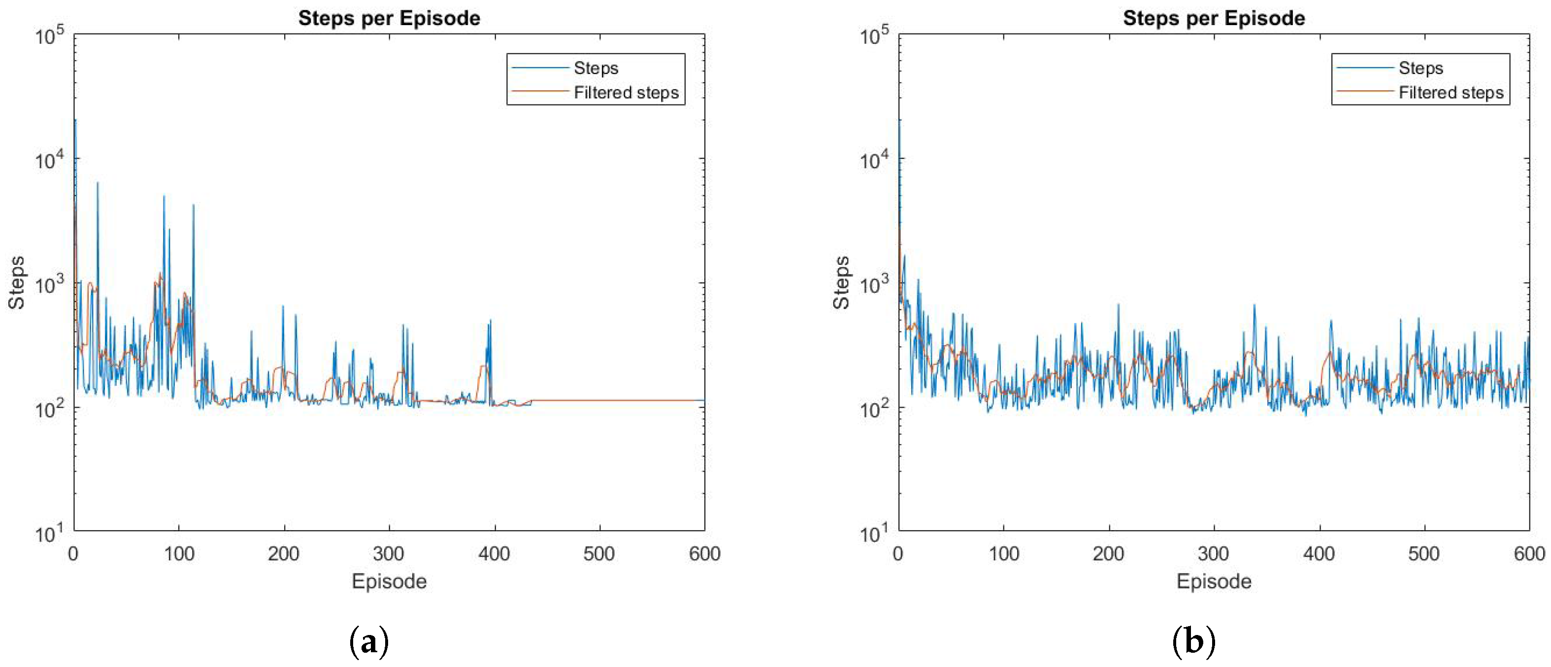
The SARSA algorithm was tested ten times in each experiment in order to obtain significant results of each one. Four experiments were compared: the SARSA algorithm with no error on sensors and having the matrix initialized with zero values; with an added error of to the output of the sensors; having the matrix initialized with non-zero values; with an added error and having initialized with non-zero values. The results are depicted in Figure 2.
Those experiments which have an added error (Figure 2b,d) do not converge, but in this case the algorithm is more robust to changes. Those controllers that do not have an added error (Figure 2a,c) converge without any noise. In the case of the random initialization (Figure 2c,d), it converges before, but it needs more steps to achieve the goal. Finally, the initialization with zero values (Figure 2a,b) is smoother and it takes less time to go above one meter.
4.2. PD Controller
The value of the gains for the PD controller of Spong [9] are , and . Although the range in which the population is generated by the genetic algorithm did not have negative values, the BLX- operator found better values outside this range.
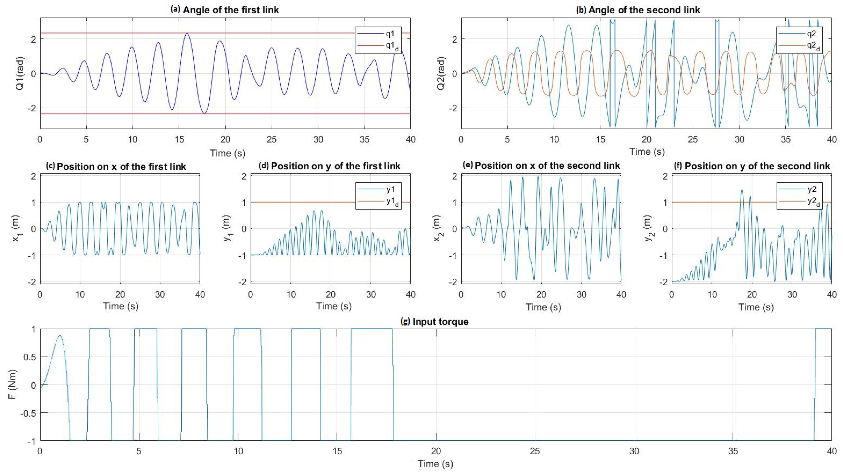
The behaviour of this controller is shown in Figure 3.
Almost all the time, the torque is saturated (Figure 3g) because of the low maximum torque. The controller lasts 13.3 s (Figure 3f) to achieve the goal, but the balancing controller should begin to control the acrobot at 17.5 s, when the red lines of the first graphic (Figure 3f) are exceeded (those lines are at and ). Fortunately, at 17.5 s the acrobot is in a good position to be controlled by the balancing controller.
The conventional PD controller tuned by the genetic algorithm has the gains , and , and the results are shown in Figure 4.
The first time the controller achieves the goal is at the 18th second (Figure 4f) , but the balancing controller cannot control on that point because the red line of the first graph (Figure 4a) has not been exceeded. The conventional PD controller cannot control the acrobot, nor can the PD controller of Spong [9] with such a low maximum torque.
4.3. PWM Controller
The gains obtained by the genetic algorithm are shown in Table 2.
These gains have the same order of magnitude as the ones we expected. The negative gains are not usual in the classical control, but the genetic algorithm found that those are the best values for this problem. The result of this controller is shown in Figure 5.
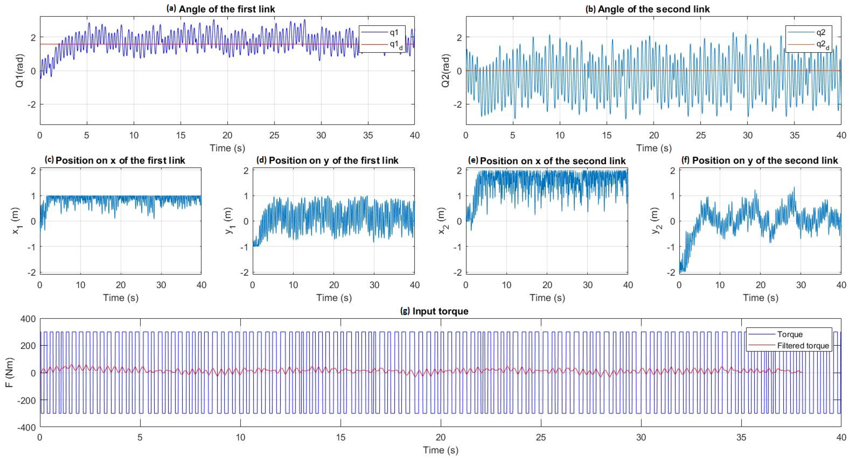
The controller takes three seconds (Figure 5a) to surpass the red line, where the balancing controller starts to handle the acrobot. Additionally, the acrobot is at a good position for the balancing problem, as the end of the acrobot is close to the two meters on the x axis (Figure 5f) and the angle of the second link is close to 0 (Figure 5b). On the second link’s position in the y axis (Figure 5f), most of the time the acrobot is above one meter, so this controller is also valid to solve the balancing problem.
Another advantage of this controller is its ability to maintain the acrobot on impossible points until now, as the and , on horizontal position (Figure 6). In this operation point, the acrobot cannot be motionless. The PWM controller can work with the two joints at the same time and control the acrobot in this point.
5. Conclusions
In this paper, we prove that the acrobot can be controlled with a very low actuation through SARSA and a modified PD, but not by a conventional PD controller. We have also explored two variants of SARSA, and we found that the algorithm with a low error is not able to converge, and the algorithm converges more quickly if the is initialized randomly, but finds worse solutions than if the initialization is with zero values.
Furthermore, we have developed a new PWM controller to control the acrobot with a large motor. This controller has large oscillations, but it lets the acrobot solve the acrobot problem in a shorter time than many approaches from the literature. With this new controller, it is also possible to maintain the acrobot in new operation points.
Moreover, we developed a genetic algorithm to tune both PD and PWM controllers, and it found the values of the controller parameters that solve the swing-up problem.
As further work, we are exploring new controllers to improve the performance our novel PWM controller, reducing the oscillations and the maximum torque needed.
Author Contributions
Two new controllers applied to the acrobot problem: PWM controller and a canonical PD; and a comparative between two variants of SARSA, two PD controllers and the novel PWM controller.
Conflicts of Interest
The authors declare no conflict of interest.
References
- Fantoni, I.; Lozano, R.; Spong, M. Energy based control of the Pendubot. IEEE Trans. Autom. Control 2000, 45, 725–729. [Google Scholar] [CrossRef]
- Boone, G. Minimum-time control of the Acrobot. Proc. Int. Conf. Robot. Autom. 1997, 4, 3281–3287. [Google Scholar]
- Brown, S.C.; Passino, K.M. Intelligent Control for an Acrobot. J. Intell. Robot. Syst. 1997, 18, 209–248. [Google Scholar] [CrossRef]
- Duong, S.C.; Kinjo, H.; Uezato, E. A switch controller design for the acrobot using neural network and genetic algorithm. In Proceedings of the 10th IEEE International Conference on Control, Automation, Robotics and Vision, Hanoi, Vietnam; 2008; pp. 1540–1544. [Google Scholar]
- Duong, S.C.; Kinjo, H.; Uezato, E.; Yamamoto, T. On the continuous control of the acrobot via computational intelligence. In Proceedings of the Lecture Notes in Computer Science (Including Subseries Lecture Notes in Artificial Intelligence and Lecture Notes in Bioinformatics), Tainan, Taiwan, 24–27 June 2009; pp. 231–241. [Google Scholar]
- Horibe, T.; Sakamoto, N. Swing up and stabilization of the acrobot via nonlinear optimal control based on stable manifold method. IFAC-PapersOnLine 2016, 49, 374–379. [Google Scholar] [CrossRef]
- Mahindrakar, A.D.; Banavar, R.N. A swing-up of the acrobot based on a simple pendulum strategy. Int. J. Control 2005, 78, 424–429. [Google Scholar] [CrossRef]
- Nichols, B.D. Continuous action-space reinforcement learning methods applied to the minimum-time swing-up of the acrobot. In Proceedings of the 2015 IEEE International Conference on Systems, Man, and Cybernetics, SMC 2015, Hong Kong, China, 9–12 October 2016; pp. 2084–2089. [Google Scholar]
- Spong, M.W. The swing up control problem for the acrobot. IEEE Control Syst. 1995, 15, 49–55. [Google Scholar] [CrossRef]
- Sutton, R.S. Generalization in reinforcement learning: Successful examples using sparse coarse coding. In Proceedings of the Advances in Neural Information Processing Systems, Denver, CO, USA, 2–5 December 1996; pp. 1038–1044. [Google Scholar]
- Tedrake, R.; Seung, H.S. Improved dynamic stability using reinforcement learning. In Proceedings of the International Conference on Climbing and Walking Robots (CLAWAR), Paris, France, 25–27 September 2002; pp. 341–348. [Google Scholar]
- Ueda, R. Small implementation of decision-making policy for the height task of the acrobot. Adv. Robot. 2016, 30, 744–757. [Google Scholar] [CrossRef]
- Wiklendt, L.; Chalup, S.; Middleton, R. A small spiking neural network with LQR control applied to the acrobot. Neural Compu. Appl. 2009, 18, 369–375. [Google Scholar] [CrossRef]
- Yoshimoto, J.; Ishii, S.; Sato, M.A. Application of reinforcement learning to balancing of acrobot 3 Nara Institute of Science and Technology 33 ATR Human Information Processing Research Laboratories. Sci. Technol. 1999, 5, 516–521. [Google Scholar]
- Zhang, A.; She, J.; Lai, X.; Wu, M. Global stabilization control of acrobot based on equivalent-input-disturbance approach. Control 2011, 44, 14596–14601. [Google Scholar] [CrossRef]
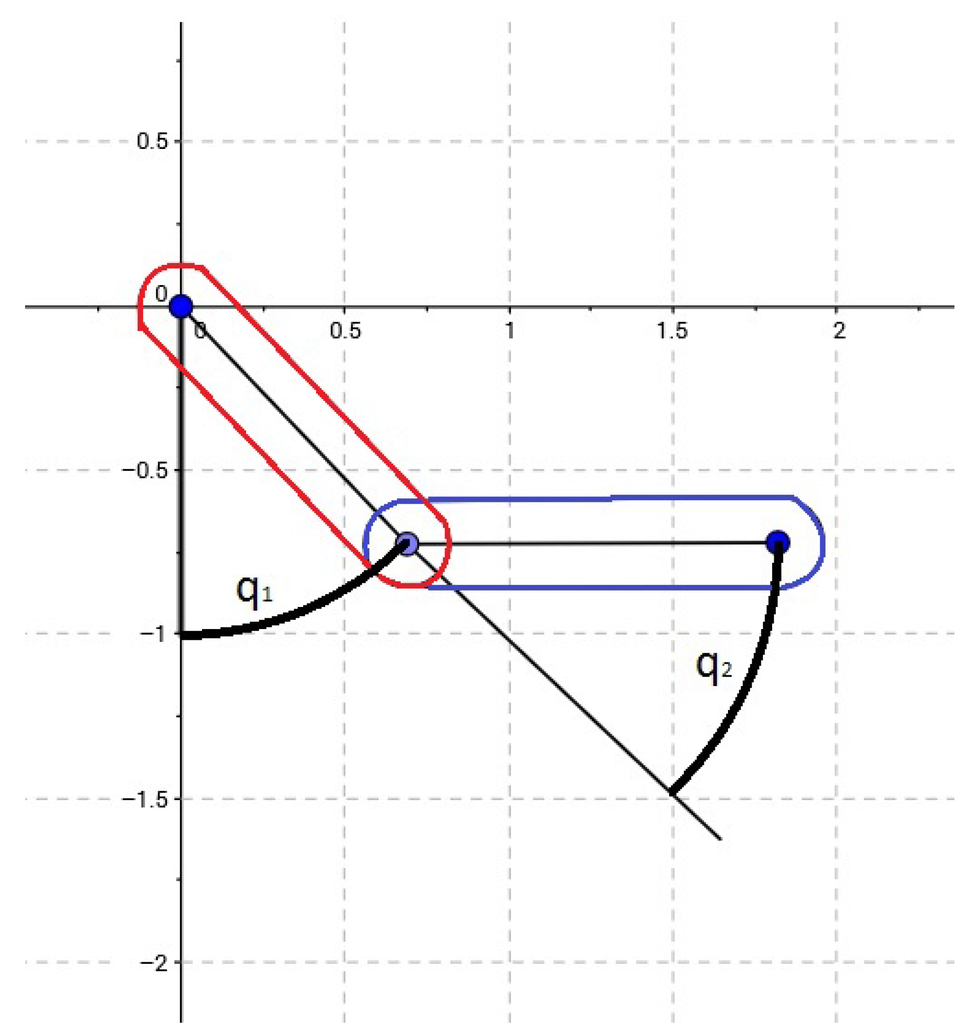
Figure 1.
Image of a simulated acrobot. This robot has a passive actuator on the first joint (on red). The second joint is on blue. The angle of the first link is called and the angle of the second link is .
Figure 1.
Image of a simulated acrobot. This robot has a passive actuator on the first joint (on red). The second joint is on blue. The angle of the first link is called and the angle of the second link is .

Figure 2.
State-Action-Reward-State-Action (SARSA) graphs of the learning rates. In each episode (x axis), the acrobot starts in the rest position. The acrobot lasts k steps (y axis) to solve the swing-up problem. If the value of steps is lower on a higher episode, the algorithm is learning. (a) With no error and zero initialization; (b) With error and zero initialization; (c) With no error and random initialization; (d) With error and random initialization. Graphs (a,c) have no error in the measured values, while (b,d) have an added error of of the range in all dimensions. (a,b) are initialized with zero values, but (c,d) are randomly initialized. The graph on the y axis is on a logarithmic scale.

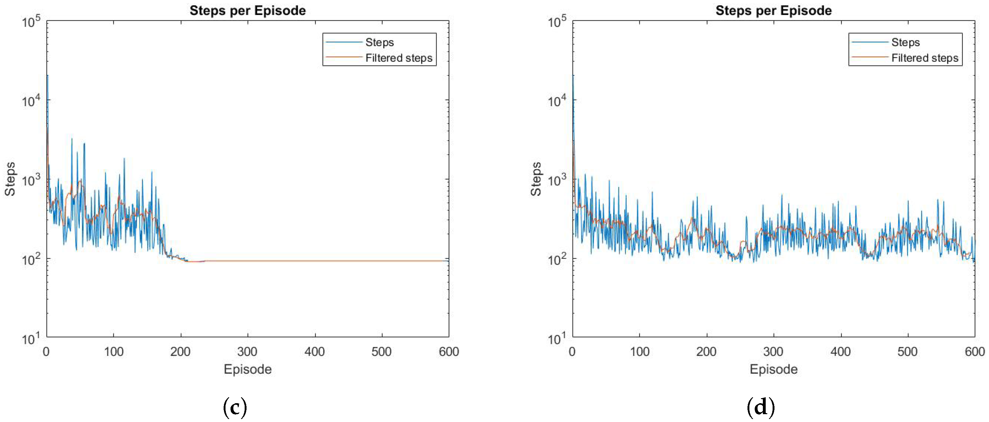
Figure 3.
Results of the proportional–derivative (PD) controller by Spong to the swing-up problem. In the first row, the positions of the angle of the first (a) and the second (b) joints are shown in radians. The red line in (a) is the moment when the other controller starts to control for the balancing problem. The red line in (b) is the desired angle of the second link. In the second row, there are the positions on x (c) and y (d) of the first link and on x (e) and y (f) of the second link. The red lines in (d) and (f) are the goal height (1 m) of the swing-up problem. In the last row, the input torque is represented (g).
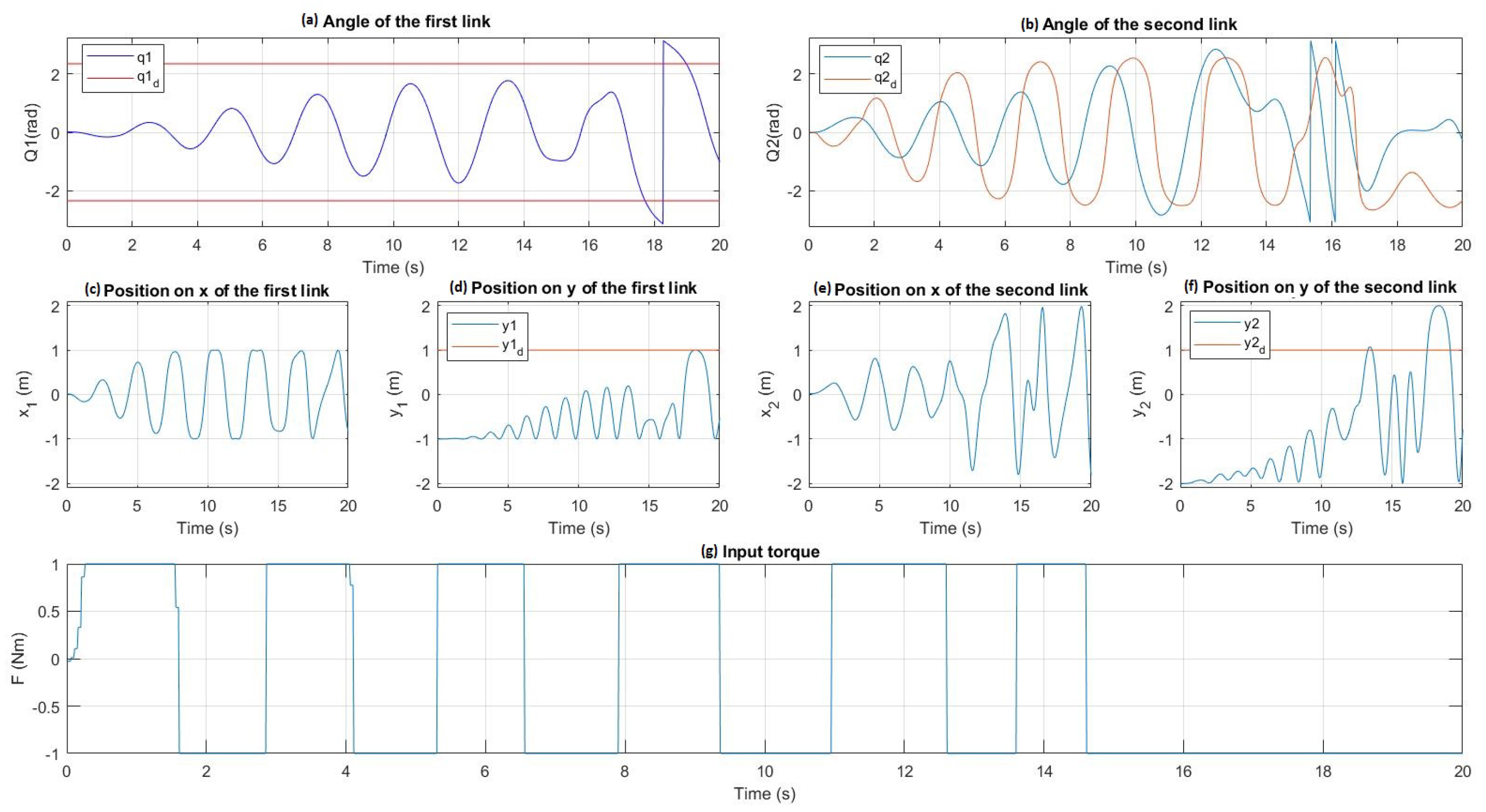
Figure 4.
Results of the conventional PD controller to the swing-up problem. In the first row, the positions of the angle of the first (a) and the second (b) links are shown in radians. The red line in (a) is the moment when the balancing controller starts to control for the balancing problem. The red line in (b) is the desired angle of the second link. In the second row, there are the positions on x (c) and y (d) of the first link and on x (e) and y (f) of the second link. The red lines in (d) and (f) are the goal height ( m) of the swing-up problem. In the last row, the input torque is represented (g).

Figure 5.
Results of the pulse-width modulation (PWM) controller to solve the acrobot problem. In the first row, he positions of the angle of the first (a) and the second (b) links are shown in radians. The red line in (a) is the moment when the balancing controller starts to control for the balancing problem. The red line in (b) is the desired angle of the second link. In the second row, there are the positions on x (c) and y (d) of the first link and on x (e) and y (f) of the second link. The red lines in (d) and (f) are the goal height (1 m) of the swing-up problem. In the last row, the graph (g) shows in blue the applied torque of the motor, and in red the same torque after a low-pass filter (the average of 10 values). By this method, it is possible to see the effect of the PWM, changing the frequency of the input signal.
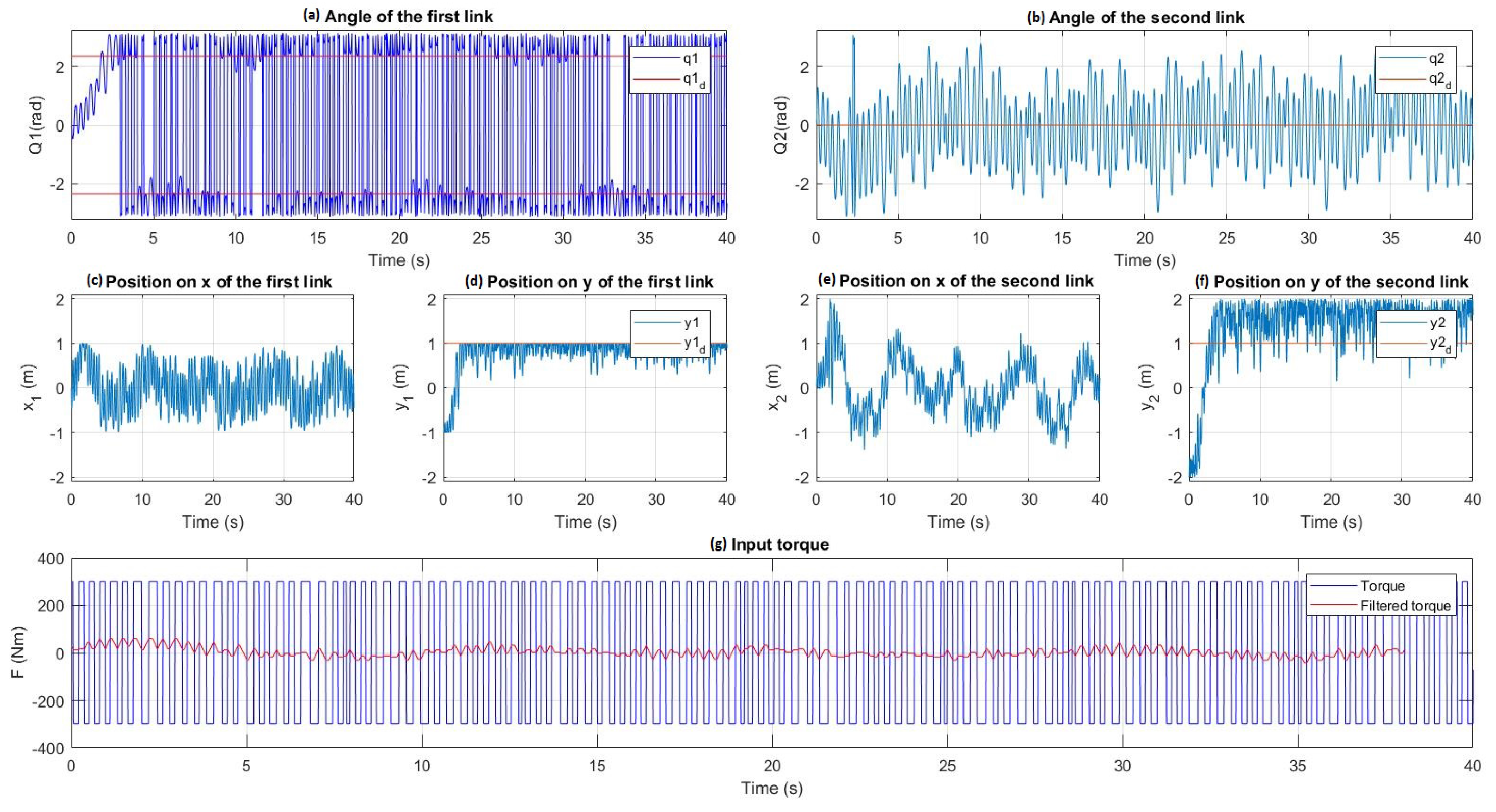
Figure 6.
Results of the PWM controller to maintain the acrobot horizontal. In the first row, the positions of the angles of the first (a) and the second (b) links are shown in radians. The red line in (a) is the moment when the balancing controller starts to control for the balancing problem. The red line in (b) is the desired angle of the second link. In the second row, there are the positions on x (c) and y (d) of the first link and on x (e) and y (f) of the second link. The red lines in (d) and (f) are the goal height (1 m) of the swing-up problem. In the last row, the input torque is represented (g).


Table 1.
Parameters of the acrobot.
| Parameters | Real Value | Meaning of the Parameter |
|---|---|---|
| 1 kg | Mass of the first link | |
| 1 kg | Mass of the second link | |
| 1 m | Distance from the beginning to the end of the first link | |
| 1 m | Distance from the beginning to the end of the second link | |
| 0.5 m | Distance from the beginning to the center of mass of the first link | |
| 0.5 m | Distance from the beginning to the center of mass of the second link | |
| 1 kg × m2 | Inertia of the first link | |
| 1 kg × m2 | Inertia of the second link | |
| g | 9.8 m/s2 | Gravity |
Table 2.
Value of the gains of the PWM controller.
© 2017 by the authors. Licensee MDPI, Basel, Switzerland. This article is an open access article distributed under the terms and conditions of the Creative Commons Attribution (CC BY) license (http://creativecommons.org/licenses/by/4.0/).
Share and Cite
MDPI and ACS Style
Mier, G.; Lope, J.D. Control of the Acrobot with Motors of Atypical Size Using Artificial Intelligence Techniques. Inventions 2017, 2, 16. https://doi.org/10.3390/inventions2030016
AMA Style
Mier G, Lope JD. Control of the Acrobot with Motors of Atypical Size Using Artificial Intelligence Techniques. Inventions. 2017; 2(3):16. https://doi.org/10.3390/inventions2030016
Chicago/Turabian StyleMier, Gonzalo, and Javier De Lope. 2017. "Control of the Acrobot with Motors of Atypical Size Using Artificial Intelligence Techniques" Inventions 2, no. 3: 16. https://doi.org/10.3390/inventions2030016