Frequency-Domain Joint Motion and Disparity Estimation Using Steerable Filters


1
Department of Electrical & Computer Engineering, Democritus University of Thrace, University Campus Xanthi-Kimmeria, 67100 Xanthi, Greece
2
Department of Electrical & Electronic Engineering, Imperial College of London, Exhibition Road, London SW7 2AZ, UK
*
Author to whom correspondence should be addressed.
Inventions 2018, 3(1), 12; https://doi.org/10.3390/inventions3010012
Submission received: 28 November 2017
/
Revised: 31 January 2018
/
Accepted: 3 February 2018
/
Published: 6 February 2018
(This article belongs to the Special Issue Innovation in Machine Intelligence for Critical Infrastructures)
Abstract
:In this paper, the problem of joint disparity and motion estimation from stereo image sequences is formulated in the spatiotemporal frequency domain, and a novel steerable filter-based approach is proposed. Our rationale behind coupling the two problems is that according to experimental evidence in the literature, the biological visual mechanisms for depth and motion are not independent of each other. Furthermore, our motivation to study the problem in the frequency domain and search for a filter-based solution is based on the fact that, according to early experimental studies, the biological visual mechanisms can be modelled based on frequency-domain or filter-based considerations, for both the perception of depth and the perception of motion. The proposed framework constitutes the first attempt to solve the joint estimation problem through a filter-based solution, based on frequency-domain considerations. Thus, the presented ideas provide a new direction of work and could be the basis for further developments. From an algorithmic point of view, we additionally extend state-of-the-art ideas from the disparity estimation literature to handle the joint disparity-motion estimation problem and formulate an algorithm that is evaluated through a number of experimental results. Comparisons with state-of-the-art-methods demonstrate the accuracy of the proposed approach.
1. Introduction
Three-dimensional reconstruction of dynamic scenes [1] and 3D scene-flow [2] estimation are important tasks in the fields of multimedia and computer vision, with numerous applications. Although active depth cameras, such as Time-Of-Flight (TOF) cameras and active IR stereo pairs, introduced new potentials in these fields and hundreds of relevant papers appeared during the last decade (e.g., [3,4,5]), the use of passive RGB cameras and passive computer vision is always an active research topic, since it holds the potential to provide richer geometric representations (due to the high resolution of passive cameras), at lower cost and without capturing limitations (e.g., only indoor environments and short capturing distances).
Scene flow was introduced in [2] as a dense 3D motion field, i.e., a field of 3D velocity vectors associated with each 3D point of a scene. Given a stereo pair with known camera calibration data, the estimation of the disparity/depth map between the image pairs and the optical flow between consecutive images is an equivalent representation of partial 3D scene flow. The problem of disparity estimation has been extensively studied during the last few decades [6,7]. Similarly, 2D motion (optical flow) estimation from monocular image sequences has been largely studied [6,8,9,10]. However, most of the existing approaches treat depth and motion independently of each other. The objective of the current work is to formulate an efficient algorithm for estimating the depth and motion in stereoscopic image sequences, by coupling and solving jointly the two problems, in order to take advantage of the spatiotemporal redundancies existing in multi-view sequences.
Specifically, in this paper, the joint estimation problem is formulated in the frequency-domain, and a steerable filter-based [10,11] approach is proposed. The motivation behind this direction of work was that early experimental studies have shown that the biological visual mechanisms can be modelled based on the spatiotemporal frequency-domain or filter-based considerations, for both the perception of depth [12,13] and the perception of motion [14,15]. Additionally, according to strong experimental evidence [16,17], the biological visual mechanisms for depth and motion are not independent of each other.
The paper is organized as follows. In Section 1.1, previous relevant works on disparity-motion estimation are reviewed, while in Section 1.2, our contributions are summarized. Section 2 provides our theoretical developments on frequency-domain joint depth-motion estimation and the construction of steerable filters for this task. The proposed algorithmic developments are given in Section 3, while experimental results are presented in Section 4, before concluding.
1.1. Previous Relevant Work
As stated, disparity estimation is an extensively-studied problem, and the corresponding literature is long, e.g., [6,7,18,19,20,21], just to name a few works. According to [7], many of them can be decomposed into a set of distinct generic steps: calculation of a pixel-wise matching-cost, cost aggregation and spatial regularization-optimization. For example, in [18], the pixel-wise matching step is based on the mutual information [22] measure, while semi-global optimization is proposed as an efficient approximation to global cost aggregation. This method [18] was selected in our experimental section, as a state-of-the-art representative of disparity-only estimation methods. Other methods are based on the extraction of sparse correspondences using local invariant descriptors (e.g., SIFT features) and a correspondence “growing” process, initialized with an “affine seed” [19,23].
In this paper, a method that estimates both disparity and flow from a stereo image sequence is proposed. Thus, the current subsection focuses on disparity plus flow estimation approaches. In general, most relevant works solve the two problems sequentially. Only, a few recent works try to solve the two problems concurrently, with probably the most notable ones the variational approaches of Huguet et al. [24] and Valgaerts et al. [25] and the “seed-growing” method of Cech et al. [26].
In [27], the 2D flow problem is first solved, and the motion information is then used during the disparity estimation step. The flow is extracted in a multi-resolution matching framework, using Gaussian pyramids. Edge features, based on the Laplacian of Gaussian, are used for this task. Disparity estimation is then performed using dynamic programming to minimize a specific cost function. Similarly, in [28], disparity and motion estimation is completed in two sequential stages: The disparity field is initially estimated by iteratively minimizing a specific cost function. Then, using a similar iterative algorithm, two dense velocity fields for the left and right stereo images, as well as the disparity field for the next time instance are estimated.
A recent, sophisticated method, more relevant to our work, due to its steerable filter implementation (though in the original spatiotemporal domain), can be found from Sizintsev et al. [29]. An accurate 3D motion and disparity model is formulated in the spatiotemporal domain, which is used to derive “spatiotemporal orientation correspondence constraints”. The disparity is initially estimated via matching of spatiotemporal quadric elements (“stequels”), calculated using 3D second-Derivatives Of Gaussian (DOG) filters. Given the disparity estimates, the matched “stequels” support recovery of scene flow estimates. The methodology is improved by the same authors in [30].
In contrast to the above approaches, which estimate motion and disparity sequentially in two stages, the authors in [31] introduce a joint estimation framework, based on a probabilistic model. The model is a Markov Random Field (MRF) whose label space, apart from velocities and disparity, incorporates also an “occlusion status” for every pixel. The problem is finally cast as an objective function minimization problem, with a NSSD (Normalized Sum of Squares Difference) data-term and a smoothness-term (“continuity” cost), which is minimized using the min-sum formulation of loopy belief propagation.
Similarly, the method in [24] estimates disparity and motion in a single optimization procedure. The use of a variational framework allows one to properly handle discontinuities in disparity and motion, as well as occlusions. The method introduces also a global energy function, which consists of data terms based on the images’ intensities and gradients’ differences, as well as regularization terms for the left/right flows and the disparities in two consecutive frames. In order to solve the non-linear differential equations that arise by the consideration of the specific energy function, an incremental multi-resolution algorithm is proposed. The method in [32] is based on similar ideas. The disparity for the first frame is initially estimated by a state-of-the-art hybrid stereo approach, more specifically using an over-segmentation-based method [33], and then refined by a hierarchical (coarse-to-fine) loopy belief propagation. Using the initial estimate of disparity, the flow and disparity for the next frame are estimated using a variational method, similar to that of [24]. The authors in [32] calculate also an associated confidence map, which is incorporated into the stereo model for the next time instance as a soft constraint.
Similarly to most approaches in the literature [7], all the previous reported methods assume a stereo pair in parallel configuration or equivalently a rectification preprocessing step. In contrast, the method in [25] assumes a general stereo geometry, i.e., the stereo fundamental matrix [34] is unknown. Since the stereo geometry is unknown, apart from the pixel-wise left/right flows and disparity, there are seven additional unknowns to be found. The method introduces a global energy function, which combines the spatial and temporal information of the different views, while imposing geometric consistency. The specific energy, in its initial formulation, is difficult to minimize, because it includes a quadratic expression with respect to the optical flow. However, the authors obtain an approximate linear expression and use a coarse-to-fine approach.
The described methods more-or-less are based on the iterative minimization of a certain cost function, which incorporates global smoothness constraints. These methods are far from real time (e.g., the reported runtime in [25] is of the order of hundreds of seconds). A recent work that addresses computational efficiency is presented in [35], where a variational framework is also used. However, to achieve computational efficiency, the authors propose to treat separately the disparity and optical flow problems.
To obtain much faster performance, a completely different approach is followed in [26], where a “Growing Correspondence Seeds for scene Flow” (GCSF) algorithm is proposed to jointly estimate disparity and flow. The idea of “seed growing”, which as stated was initially adopted in stereo [19], is based on the basic principle that a set of sparse correspondences is established between images (stereo pairs and/or consecutive frames), and these “seeds” are then propagated to their neighbourhood. The advantage of such approaches is a faster performance compared to global variational and MRF methods and a good accuracy compared to purely local methods. Additionally, the GCSF approach [26] naturally preserves the boundaries between objects, without introducing smoothing artefacts. The algorithm produces semi-dense results, which are however dense enough for several potential applications. According to the experimental results in [26], the method produces more accurate results compared to the variational algorithm of Huguet et al. [24] and the spatiotemporal stereo algorithm by Sizintsev et al. [30]. The GCSF method [18] was selected in our experimental section, as a state-of-the-art representative of joint disparity-flow methods.
Other recent methods [36,37], targeting more specific applications, propose novel multi-frame methods for computing the 3D structure and motion of a scene, as observed from a stereo camera rig on a moving vehicle. The work in [36] is based on the assumption that the captured scene is static; only the stereo rig moves. A semi-global matching [18] approach is exploited to independently compute a disparity and a flow field from the stereo and the motion pairs, respectively. These are then used to estimate a scaling relationship between stereo and flow, assuming that the scene is static and thus the relationship between the two fields is constant (across pixels). In the next phase, given this constant relation, the two fields are jointly optimized. The estimated maps then feed a proposed slanted-plane method, which infers image segmentation, a slanted plane for each segment and an outlier flag for each pixel. The method is based on the minimization of an objective function with: (i) an energy term that prefers well-shaped, compact segments; (ii) an “appearance” term that encourages pixels of with a similar colour to belong to the same segment; (iii) a “disparity” term that forces the plane estimates to explain the estimated depth well; (iv) a term that encourages the planes of adjacent segments to be similar; and (v) a term that encourages straight/smooth segments’ boundaries. The specific cost function is complex, and its minimization is an NP-hard problem; however, the authors derive a simple, yet effective descent optimization algorithm, much faster than other methods. The work in [37] goes one step further and targets additionally the estimation of the non-rigid motion of foreground moving object regions. It similarly begins with the assumption that the dominant scene motion is rigid (i.e., due to only the six-degree-of-freedom stereo-rig motion), and thus, the optical flow for the stationary 3D points is constrained by their depths. Therefore, initially, the disparity and the camera motion are estimated using stereo matching and visual odometry techniques. Foreground moving object regions (“flow outlier”) are then detected, and optical flow is performed only for these regions. The resulting non-rigid flow is fused with the rigid one to obtain the final flow and segmentation map.
Finally, although not completely relevant, another set of methods [38,39] should also be mentioned here, which make use of disparity cues (apart from appearance cues) to obtain pixel-wise segmentation and pose estimation of multiple specific-class deforming objects, such as humans, in stereoscopic videos. For example, the work in [39] estimates an approximate disparity map on a per-frame basis, which along with colour (appearance) cues is incorporated in a novel segmentation model that make use of person detections and learnt articulated pose segmentation masks. The method’s output is a layered representation of humans in a scene, where each person is assigned a different depth layer. It manages to handle challenging scenarios in complex indoor and outdoor dynamic scenes.
1.2. Summary of Contributions
In this paper, we aim at formulating a steerable filter-based approach that is based on a frequency-domain considerations and tries to solve simultaneously the two tasks by minimizing a single energy function. According to the best of the authors knowledge, this is the first effort to formulate the joint estimation problem in the frequency domain and to provide an efficient filter-based solution. Thus, the presented ideas provide a novel direction of work and could constitute the basis for further developments. The experimental results given in this paper and comparisons with state-of-the-art-methods [18,26] demonstrate the accuracy of the proposed approach.
The main contributions of this paper can be summarized as follows:
- Theoretical foundations for frequency-domain joint depth and motion estimation are given. Additionally, the construction of spatiotemporal steerable filters in the frequency domain, appropriate for the joint estimation task, is presented.
- Based on the above theoretical developments, a novel algorithm for joint disparity and motion estimation is formulated. Due to the computational efficiency of the steerable filters, the proposed method presents relatively low computational effort given the high complexity of the problem, while it is appropriate for parallel GPU implementation.
- To the best of the authors knowledge, the proposed approach constitutes the first attempt towards simultaneous depth and motion estimation using frequency-domain considerations. The presented ideas provide a novel paradigm for frequency-domain, filter-based coupled disparity-motion estimation and could constitute the basis for new developments.
- Finally, in the proposed algorithm, the semi-global scan-line optimization approach for stereo matching [18] is extended and successfully applied in the joint motion-disparity estimation problem.
2. Theoretical Developments
2.1. Motion and Disparity Model in the Frequency Domain
We consider the typical pinhole-camera perspective projection model [6,34] and assume that the input stereo image data are rectified [7].
Consider a 3D point/small 3D neighbourhood that moves with 3D velocity . Studying the motion locally in time around t, according to fundamental physics laws, the velocity can be considered as almost constant, i.e., . Spatiotemporally-piecewise smooth flow is a common assumption in most relevant flow estimation algorithms. The 3D point projects on the 2D points and on the left and right 2D imaging planes, respectively, with:
is the disparity vector and , b stand for the cameras’ focal length and the stereo baseline, respectively. Based on the assumption that is relatively small, the projected point on the left and right images is given by: and .
Making use of the previous facts, the projected images are locally described by:
where and stand for the left and right images and is the first frame of the left sequence.
2.1.1. Model in the Frequency Domain
Taking the 3D spatiotemporal Fourier Transform (FT) of (2), one concludes that:
where is the 2D spatial frequency, the temporal frequency and denotes the delta function, while:
The energy in the spatiotemporal frequency domain is concentrated along a “motion plane” , for both the left and right sequences. The spatiotemporal FTs have only a phase difference equal to . The “motion plane” is perpendicular to the unit vector:
2.1.2. Definitions of Energy Functions for Joint Motion-Disparity Estimation
The detection of the “motion plane” along with the phase can give an estimate of both flow and disparity. Making use of (3), we have:
Based on this, the following energy functions can be introduced:
where:
denotes the FT of . Observing that , one deduces that is maximized for equal to the actual 2D velocity and D equal to the actual disparity. Intuitively, for D equal to the actual disparity, and are in phase for each spatiotemporal frequency , and therefore, their sum is maximized. Similarly, the energy functional is minimized at D equal to the actual disparity.
2.2. Steerable 3D Filters for Joint Motion-Disparity Estimation
In [10], a complete framework for the construction of 3D steerable filters and their application to flow estimation can be found. In this work, we adapt and extend the relevant theory, towards the construction and use of filters for joint motion-disparity estimation.
2.2.1. Directional Filters and Filter “Replicas”
A directional filter of order N, oriented along the unit vector in the spatiotemporal frequency domain, is given from , where the spatiotemporal frequency and . The filter in the original domain is notated as . For simplicity, from now on, N is dropped from the notation.
For the theoretical developments of this work, we also define the filters’ “replicas”, shifted along the horizontal direction x:
where .
With denoting an image sequence and its representation in the 3D frequency domain, the response of a directional filter is notated as and in the original and the frequency domain, respectively.
It is straightforward to show that the response of a shifted filter equals the shifted response of the original filter, i.e., and .
2.2.2. “Steerability” Property
A directional filter can be “interpolated” from basic directional filters , namely:
where denote the interpolation coefficients [10].
Based on the definition (9), it can be shown that the same interpolation formula holds for the filter replicas, namely . It is obvious also that due to the linearity of FT, the interpolation formula holds in the original space-time domain. Additionally, the formula holds for the filter responses and the responses of their replicas, i.e., .
2.3. Definition of Appropriate Energy Functions
The “donut mechanism” [10,40] has been effectively applied in the 2D optical flow problem. It enables the fast calculation of an energy functional, known as the “max-steering” distribution, which describes the spectral energy distribution along (near) the motion planes. The “donut mechanism” can be summarized in the following bullets:
- Find direction vectors, notated as , that are equally distributed and lie on the candidate motion plane.
- The “max-steering” distribution is defined from:
2.3.1. Functions for Joint Motion-Disparity Estimation
Recall that the functionals and in (7) are maximized and minimized, respectively, when equals the actual 2D velocity and D is equal to the actual disparity. Inspired by these functionals, the aim here is to define appropriate extensions of the “max-steering” distribution, with a similar steerability property. Towards this end, the following combined energy functions are defined:
where denotes the shifted replica of and , denote the input stereo sequence in the frequency domain. By making use of Parseval’s property, (13) is rewritten as:
Taking into account that the responses in the original domain are either pure real or pure imaginary, after a set of manipulations, one can split the expression of (14) into:
where:
Steerability property: The definition of is exactly the same as in (11); therefore, its steerability property holds. The property holds also for and , since the complex multiplication factor does not affect the summations. Specifically, it can be shown that , and can be interpolated from a set of fixed quadratic terms:
namely:
where is given from (12) and similar equations hold for and .
2.3.2. Functions for Pixel-Wise (Local) Estimation
Since we are interested in dense motion and disparity estimation, the functions have to be modified and defined for each spatiotemporal position . The “pixel-wise” functions , and are defined by dropping the summation along in Equation (16). This modification does not affect the “steerability” property of the functions.
2.3.3. Combined Cost Function for Motion-Disparity Estimation
On the one hand, is theoretically maximized for equal to the actual velocity-disparity, and practically, it is more efficient in the motion estimation task. On the other hand, is minimized for disparity D equal to the actual disparity, regardless of the velocity; therefore, if used alone, it is useful only for disparity estimation. According to the above, and given that a cost function should be minimized at the actual velocity-disparity pair, we introduce a combined cost function, appropriate for joint motion-disparity estimation, as follows:
where . The weight w is selected equal to , where denotes the sample standard deviation.
2.3.4. Handling Responses of Shifted Filter Replicas: Sub-Pixel Accuracy
The calculation of the terms in (17) involves the responses , i.e., the responses of the shifted filters’ replicas. However, the response of a shifted filter equals the shifted response of the original filter. This practical property means that only the application of the original filters is needed. On the other hand, although shifting a 2D function in the original domain is straightforward for an integer D, shifting by an arbitrary D requires sub-pixel interpolation. One way to do that is trigonometric interpolation, i.e., multiplying in the FT domain by . Based on this discussion, we split the real-valued D into its integer part and the remaining decimal part: , where . With this definition, we have:
where and . This means that if disparity estimation with sub-pixel accuracy equal to is needed, one has to calculate for all , . For example, for quarter-pixel accuracy, .
3. Algorithmic Developments
3.1. Outline of the Main Algorithm
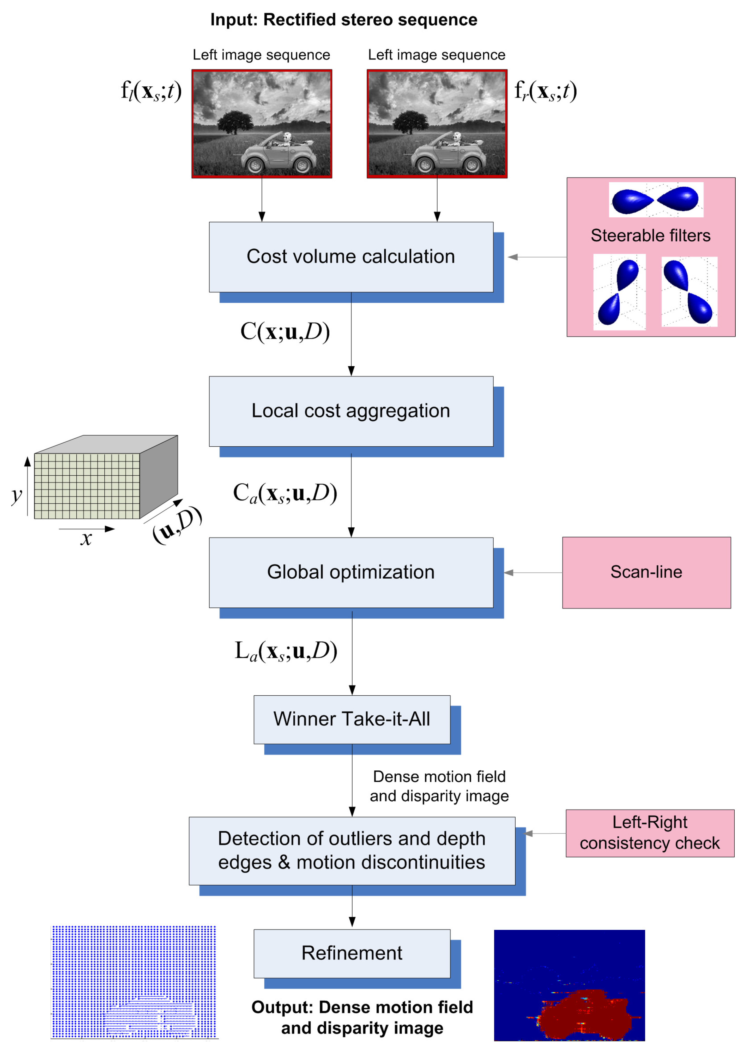
The proposed algorithm receives as input a rectified stereo image sequence of T frames ( in our experiments) and outputs a motion field and a disparity map for the middle frame (). The overall structure of the algorithm, summarized in the block diagram of Figure 1, is described by four basic “building blocks”:
- (Matching) Cost volume computation: Based on our theoretical steerable filters-based developments, this step calculates a cost hyper-volume .
- Cost (support) aggregation: The cost hyper-volume is spatially aggregated in a local region around each pixel, using a window, to produce the hyper-volume . A Gaussian window of size or and standard deviation equal to W is used.
- (Semi-)global optimization: In our case, where the cost hyper-volume is defined over the 5D (2D space + 2D velocity + disparity) space, global optimization [41] would be very slow, even with modern efficient methods, such as graph-cuts [42] or belief propagation [31]. We extend and use a semi-global optimization [18].
- Disparity-velocity refinement: This step performs refinement of the estimates, by detecting and correcting outlier estimates.
3.2. Cost Volume Calculation and Local Aggregation
3.2.1. Cost Volume Calculation
The steps for the calculation of the cost hyper-volume can be summarized as follows:
- Construct a 3D steerable filter basis in the frequency domain, at the basic orientations . This step is independent of the input sequence, and therefore, the filter basis can be constructed off-line.
- Compute the spatiotemporal FT of the input sequences to obtain and .
- Pre-processing: Since most natural images have strong low spatial-frequency characteristics, we amplify the medium-frequency components via band-pass pre-filtering, as in [10].
- Multiply and with each basic filter , to obtain the basic responses and , respectively. If sub-pixel accuracy is wanted (see Section 2.3.4), calculate also the sub-pixel shifted responses .
- Apply 3D IFT to each and to get the basic responses in the original space-time domain and . From Equation (20), the responses are available for all candidate shifts D, with the wanted sub-pixel accuracy.
- Calculate the quadratic terms , and , defined in Section 2.3.1 (Equation (17)), for each candidate disparity D.
- The quadratic terms are aggregated along the T input frames using a 1D Gaussian window , i.e., . Similar equations are used for and . Experimentally, it was found that a good choice for the extent (standard deviation) of this window is .
- Calculate the distributions , as described in Section 2.3.1 and Section 2.3.2. Then, calculate the combined cost function from (19).
3.3. Adapted Scan-Line Optimization
The proposed method, taking as input a cost volume , outputs a “regularized” cost volume , which implicitly includes smoothness constraints. We adapt a semi-global optimization method to our multi-parametric motion-disparity estimation problem, specifically the Scan-line Optimization (SO) approach [18].
The SO procedure implements cost accumulation along linear paths (scan-lines), identified by a direction . Consider the scan-line , with being at the image border and at the opposite image border. To simplify notation, we let denote the i-th pixel along the path, i.e., . Initially, we ignore the unknown velocity , and the problem reduces to disparity-only estimation. For a disparity level and a scan-line direction , the cost at the i-th pixel is recursively calculated from [18]:
where:
The regularization constraints are encoded in the penalties and .
In order to proceed, we quote our observation. Equation (22) can be written in a compact form as follows:
where the matrix defines the penalty for transition from disparity to .
To handle the joint motion-disparity problem, we use a one-to-one discrete mapping from the 3D velocity-disparity search space to the 1D space of natural numbers. Specifically, we introduce a parameter and the discrete mapping , where represents the m-th candidate velocity-disparity pair. Additionally, a symmetric penalty matrix defines the penalties for the transition from to . Using this notation, we reformulate Equations (21) and (23) as follows:
where the additional parameter controls the global smoothness constraints. The penalty in our case is split into two terms, one for disparity transition and one for velocity transition:
with and given in (23). The parameter controls the relative smoothness constraints for velocity. In order to construct the penalty matrix , one has to take into account that the optical flow vectors are not always piecewise constant, but may vary slowly in small regions. It is constructed as follows:
where is a truncation threshold, used to avoid over-smoothing of the flow-field along object boundaries and is a function that is zero for and increases with the “difference” of the velocity vectors and . We propose the use of the “angular difference” (angular error in [8]), i.e., , where is given from (5). According to [8], this metric, which is expressed in radians, is fairer compared to other ones, such as the vector’s Euclidean distance.
PSO parameters: The selection of the SO parameters in our presented experiments was roughly guided by the range and the histograms (probability density functions) of the initial cost-volume values, calculated for the experimental image sequences. The SO parameters were selected as follows: the penalties for disparity are and ; the truncation threshold in Equation (26) is rads; the relative smoothness parameter for velocity (Equation (25)) is ; and the global smoothness parameter (Equation (24)) is .
3.4. WTA, Outliers’ Detection and Refinement
Given a cost volume, , the Winner Take-All (WTA) approach searches for each pixel the parameter m that minimizes the cost, i.e., . Then, the disparity and velocity estimates for pixel are: and .
3.4.1. Outliers’ Detection, Refinement and Confidence Map
Considering as a reference the Left image of the stereo pair, the estimated flow and disparity maps are obtained. However, applying the algorithm with the right view as the reference, one computes the flow and disparity estimates , which may not be consistent with .
Detection of disparity outliers: A prevalent strategy for detecting outliers is the left-right consistency check [43], according to: , where is a threshold, set equal to pixels in our experiments. Using this consistency check, the binary outliers map is obtained. Similarly, performing the right-left check, we obtain the outliers map . The final disparity outliers map, letting , is given by the union (OR operation) of and .
Refinement of disparity map: The refinement strategy is applied on , to fill each outlier pixel with a “confident” disparity value from the neighbourhood. The employed scheme is simple; for each outlier pixel: (i) the nearest “inliers”, which lie on the same line (pixel row) or the lines above and below, are detected; and then, (ii) for all the closest inliers, the regions around them are scanned and the minimum disparity value selected. The idea of selecting the minimum disparity in the neighbourhood of the outlier is based on the fact that most outliers normally correspond to background occluded regions. The output of this refinement step, applied to the left disparity map, is denoted as .
Detection of flow outliers: The proposed left-right consistency check for the flow estimates is based on similar ideas, but the Angular Error (AE) [8] is used to measure the “difference” between two flow vectors. To measure the consistency and , we consider the 3D vectors and , where is given in (5). The consistency is checked using the AE metric, i.e., from , where the threshold was set in our experiments. Let the final flow outliers map be denoted as .
Refinement of flow field: Filling outlier pixels with respect to flow should not be based on simply assigning the smallest (in magnitude) inlier flow vector in the neighbourhood of the outlier. This is because slowly moving objects can occlude faster moving objects. Therefore, here, a simple alternative is used for filling the outlier pixels: we detect the inlier flow vectors inside a square neighbourhood ( in our experiments) of each outlier and find their median. This is then assigned to the outlier pixel.
3.5. Estimation Confidence Map
Similarly to all disparity and flow estimation techniques, the proposed algorithm produces estimates whose accuracy varies with the local characteristics of the underlying images. As practice shows, wrong estimates are mainly obtained at and near the outlier regions and , as previously defined. Thus, the following simple, but effective “confidence” measure is proposed:
where is a binary image obtained from the union of the outlier maps and , stands for the Euclidean distance of pixel to the nearest non-zero pixel in and is a distance threshold, set equal to four pixels in our experiments. This means that the confidence map is zero for the outlier pixels (non-zero pixels in ) and increases with the Euclidean distance to such pixels. For distances larger than pixels, the confidence is equal to unity. An example of such a confidence map is given in the experimental results of Section 4.2.2.
The algorithm proposed so far produces disparity and flow estimates at 100% Full Density (FD). In practical scenarios, however, “non-confident” estimates could be rejected, based on thresholding the proposed confidence map. In the experimental section, to compare with state-of-the-art approaches that do not produce estimates at 100% density, the confidence map is thresholded at various levels in the interval [0, 1].
4. Experimental Results
In this section, detailed experimental on both synthetic and natural stereo image sequences are presented. Comparative results are also given, with respect to two state-of-the art methods. Specifically, the method in [26] was selected, which jointly computes disparity and flow in consecutive stereo images, based on the notion of “Growing Correspondence Seeds (GCS)” [19]. The code, freely available from the authors, was exploited using the default parameters. Additionally, the disparity-only estimation method of [18] is used, as implemented in MATLAB’s 2017a Computer Vision toolbox (denoted as MatCVTolbx-SemiG in the rest of the paper) using the OpenCV library. The method uses mutual information for the cost measure, while it applies semi-global optimization for spatial regularization. For details, please refer to the referenced works.
4.1. Prerequisites
Implementation details, CUDA parallelization: Steps 6–8 of the initial cost calculation algorithm (Section 3.2.1) were implemented using NVidia’s CUDA. These steps are fully parallelizable on a GPU, since calculations for each (space-time location) or each are independent of each other. Additionally, the SO algorithm, which is by far the slowest part of the whole algorithm, was implemented using CUDA. Due to the recursive scanning of the pixels along each scan-line, computations can be parallelized only with respect to different candidate disparity-velocity pairs (index m; see Equation (24)).
The computational times reported in this section were obtained using a PC with an Intel i7 CPU at 2.00 GHz, 16 GB RAM and a GeForce GT750M with 384 CUDA Cores.
Evaluation metrics: The (Mean) Angular Error (M)AE [8] is used as an evaluation metric for dense flow estimation. For evaluating disparity estimation, we use the mean absolute disparity error, as well as the percentage of bad pixels [7], i.e., the percentage of pixels with absolute error greater than pixel.
4.2. Experimental Results: Artificial Sequences
4.2.1. “Car-Tree” Sequence
With the help of this simple stereo sequence, shown in Figure 2a,b, the performance is studied with respect to the filters’ order N. Specifically, the performance is studied in the case that Winner Take-All (WTA) is applied directly to the initial cost volume , i.e., all subsequent steps after Step B are omitted. In the diagrams of Figure 2c–e, the estimation error metrics with respect to N are reported. As can be verified, both the disparity and motion estimates improve as the filter order increases. This comes at the cost of increased computational effort, according to Figure 2e, where the computational cost seems to quadratically increase. However, this computational cost (Steps A, B) is an order of magnitude lower than that of SO optimization (Step C), as already stated and will be revealed by the computational-time results, provided in next sections. Thus, when high accuracy is the major objective and therefore the time-consuming SO optimization step is also applied, the use of higher order filters is suggested, since the additional computational overhead will be small. On the other hand, when mainly speed matters, the application of only Steps A and B with a low filter order is proposed. As a good trade-off between accuracy and speed, omitting SO optimization (application of Steps A, B and D) and using filters of order is suggested. In the experiments of Section 4.2.2, Section 4.3.1 and Section 4.3.2 is used, whereas in the experiment of Section 4.2.3, where only Steps A and B are applied, is used.
4.2.2. “Futuristic White-Tower” Sequence
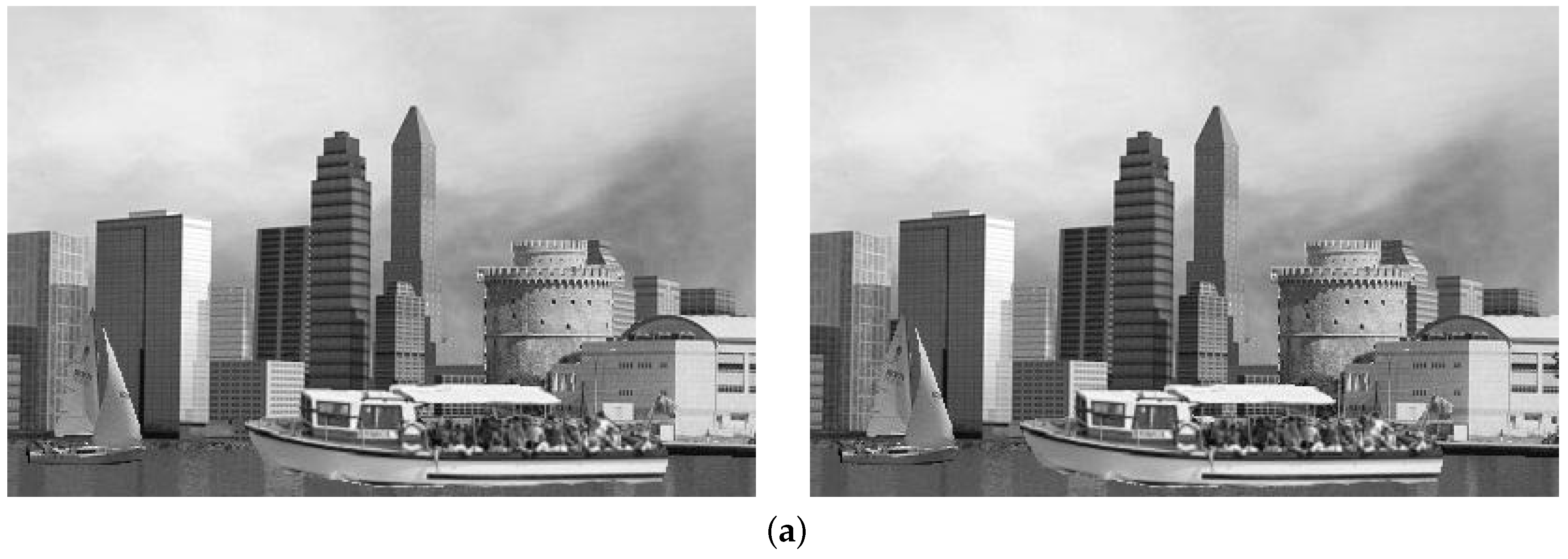
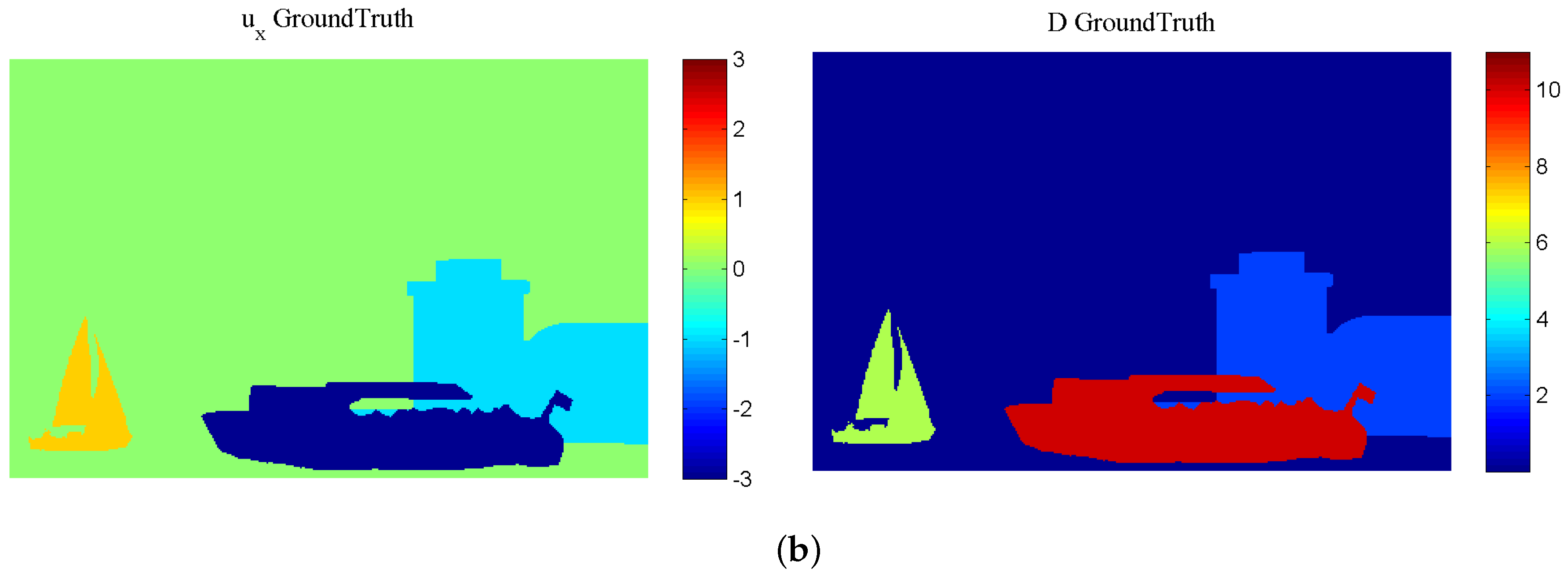
In this sequence, shown in Figure 3, apart from the very distant static background, we have three objects at different depths, with severe occlusions; from far to near: The “White-Tower” layer that moves slowly (−1 pixel/frame), simulating the motion of the virtual stereo rig, a small sailing boat (+1 pixel/frame) and a larger boat (−3 pixels/frame).
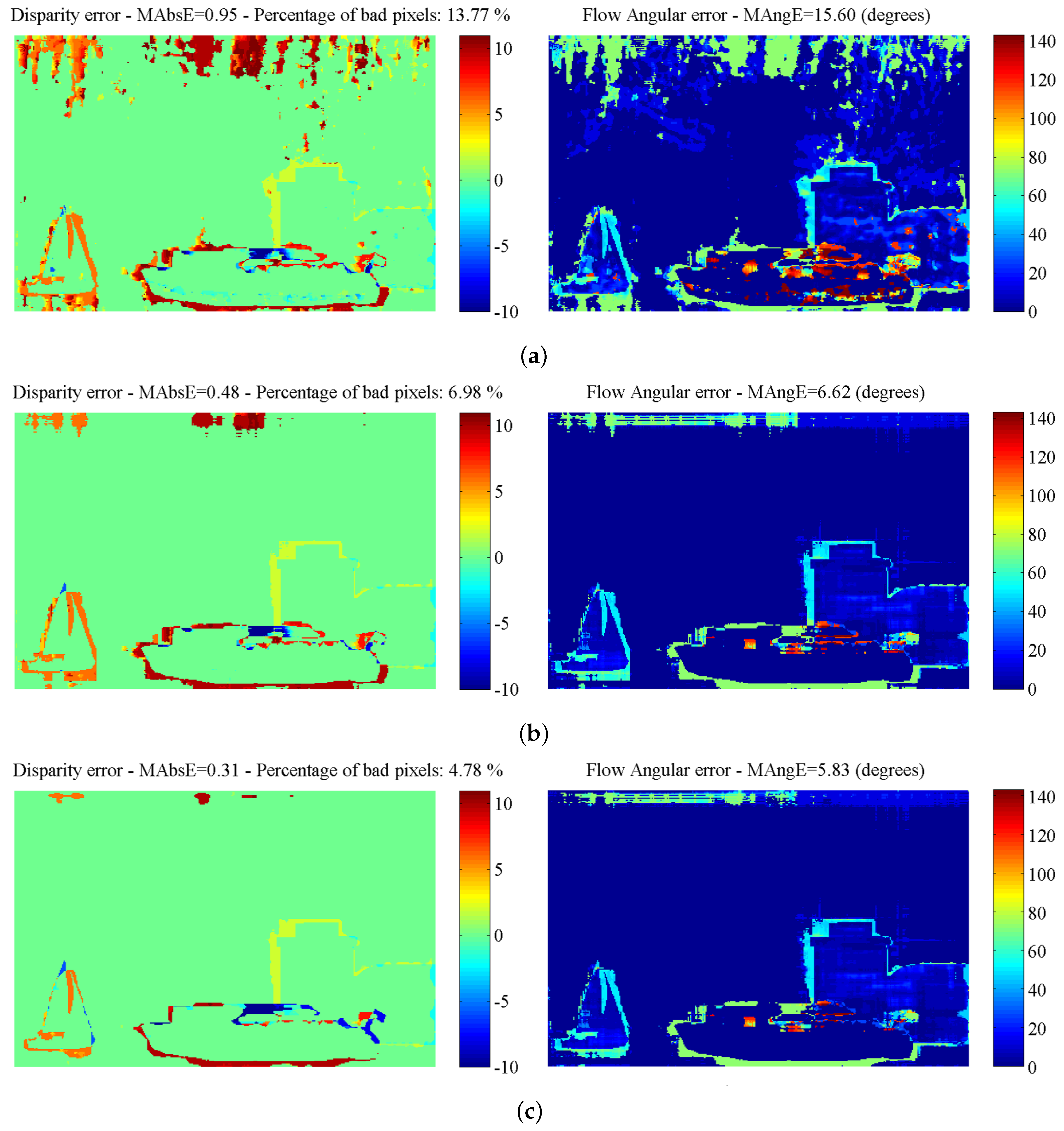
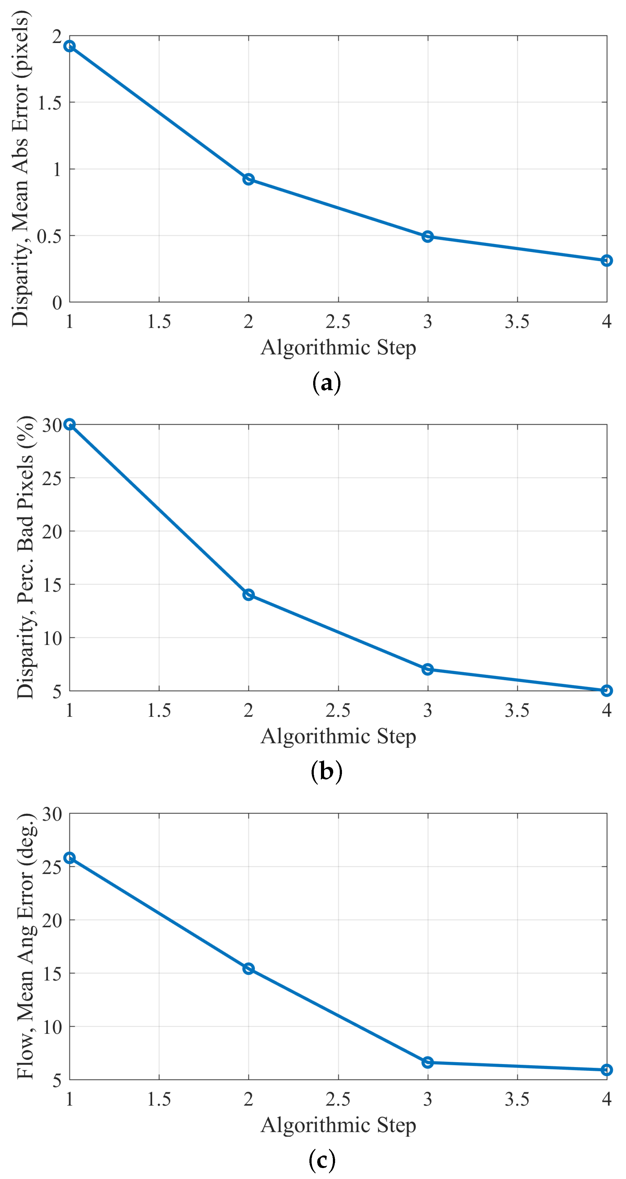
The estimation error results, at 100% FD, obtained after the application of each algorithmic step, are given in Figure 4. As can be observed, the errors occur mainly at untextured regions (e.g., the sky) and object boundaries, due to the “blank wall” and “aperture” problems [8,9]. However, after the application of the scan-line regularization step, the estimated maps become smoother, and the error at homogeneous regions is eliminated, but the error at object boundaries remains. The last step of the algorithm (outliers’ refinement) introduces improvement at the object boundaries. As can also be verified from the diagrams of Figure 5, each algorithmic step introduces an improvement.
Table 1 reports the processing time of the computationally-demanding parts, i.e., with the initial cost volume calculation and the scan-line optimization, considering both a CPU and a GPU implementation. Although the calculation of the initial cost volume is quite fast (Steps A and B), scan-line optimization (Step C) is slower by approximately an order of magnitude, due to the last parametric search space (disparity and 2D motion). A GPU implementation of these steps can speed-up execution by a factor of approximately four.
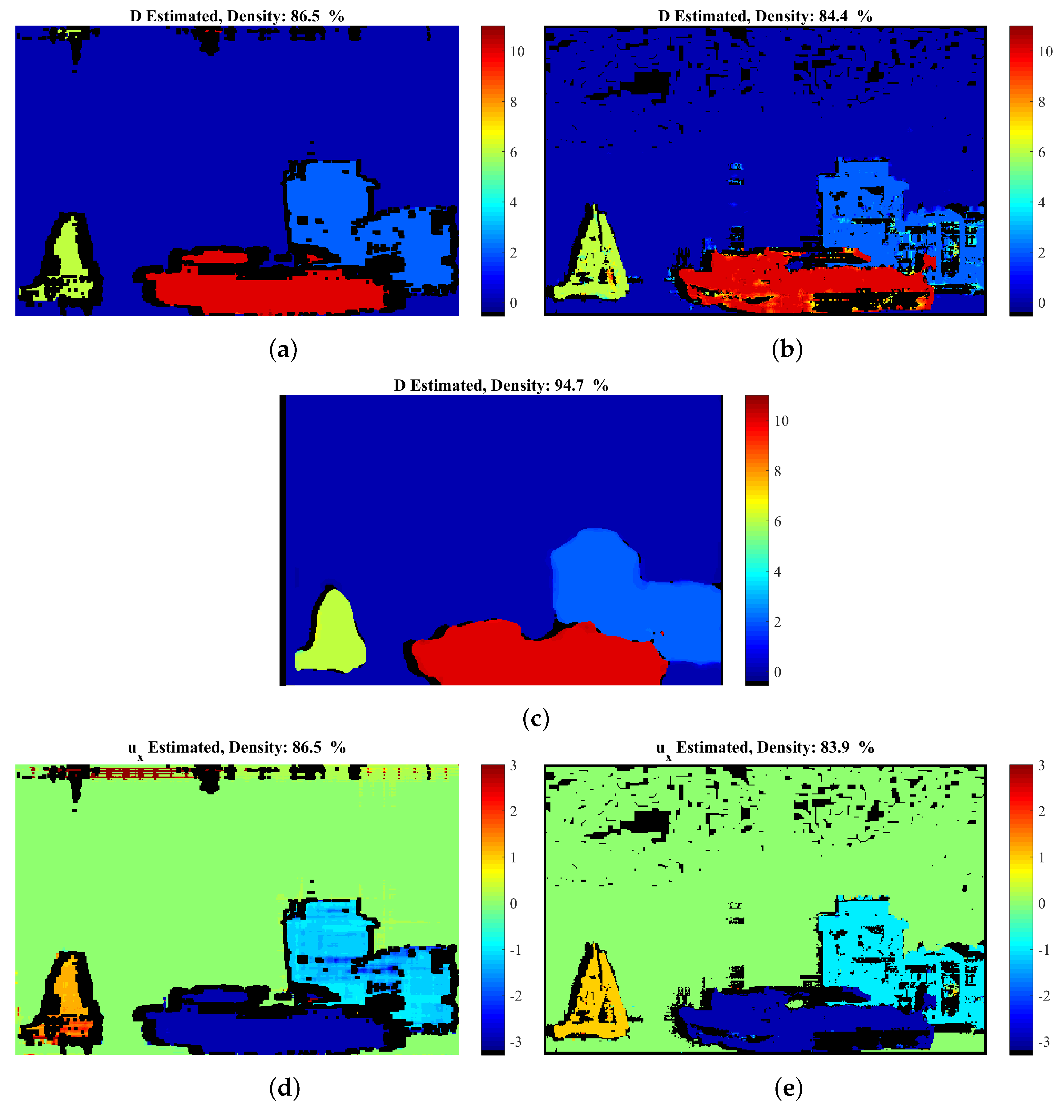
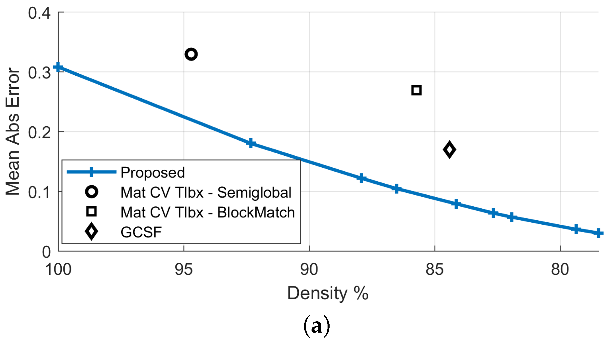
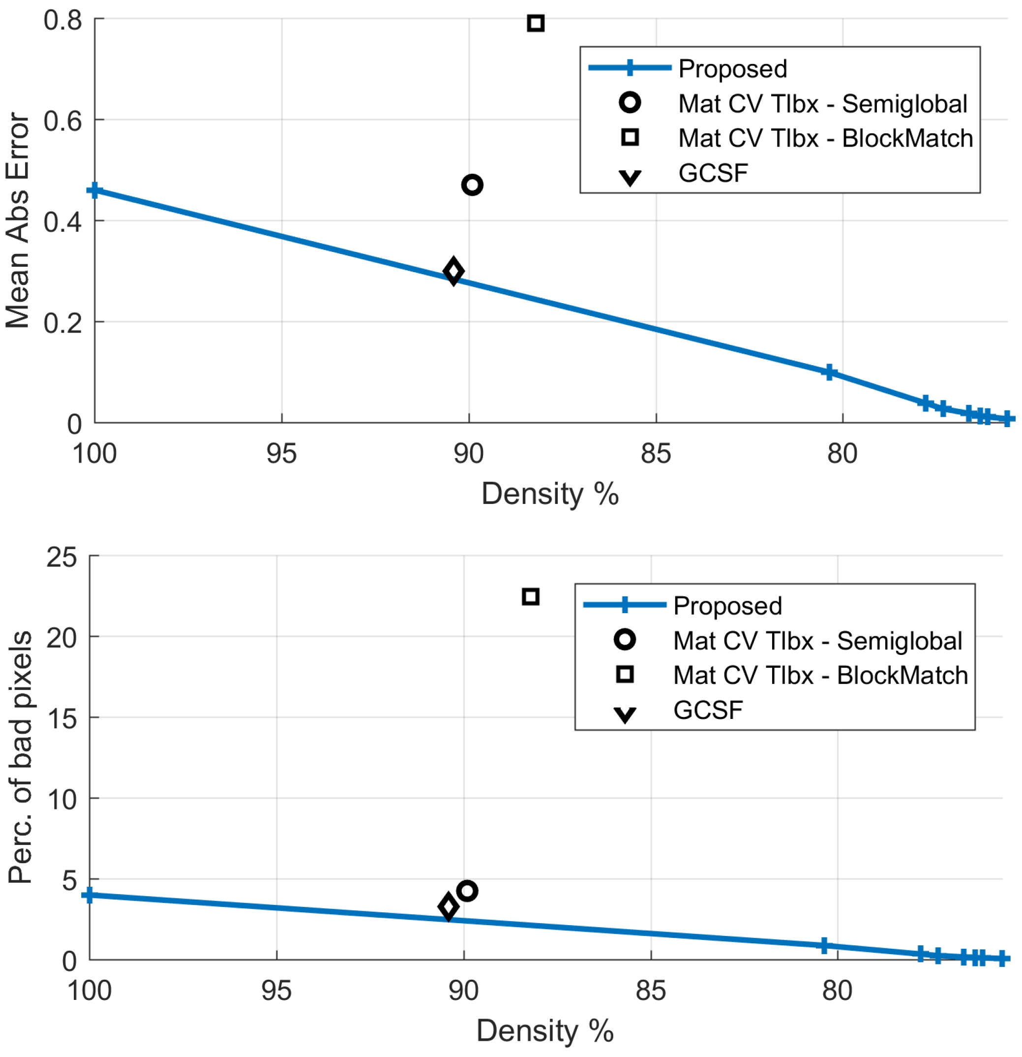
The confidence map, calculated as described in Section 3.4.1, is given in Figure 6. The proposed method’s density is varied by thresholding this confidence map in the interval [0, 1]. Comparative results against the GCSF ([19,26]) and the MatCVTolbx ([18]) methods are given in Figure 7 and Figure 8, as well as in Table 2. According to Table 2 and Figure 8a,b, the proposed method outperforms the other methods with respect to disparity estimation, producing estimates at similar or higher densities with lower Mean Absolute Error (MAbsE) and Perc.of bad pixels. According to Figure 7c, the MatCVTolbx method oversmooths the results, producing erroneous estimates at object boundaries (“edge-fattening” effect). According to Figure 7a,b, the behaviours of the proposed method and GCSF are similar, regarding the “rejected” estimates, which are concentrated near object boundaries and at the textureless sky region. Similar conclusions are drawn from Figure 7d,e, which depicts the corresponding estimated flow maps (horizontal component). The methods produce flow estimation results with similar Mean Angular Error (MAngError), at similar densities, as can be verified from Table 2 and Figure 8c.
4.2.3. “Rotating Lenna Plane” Sequence
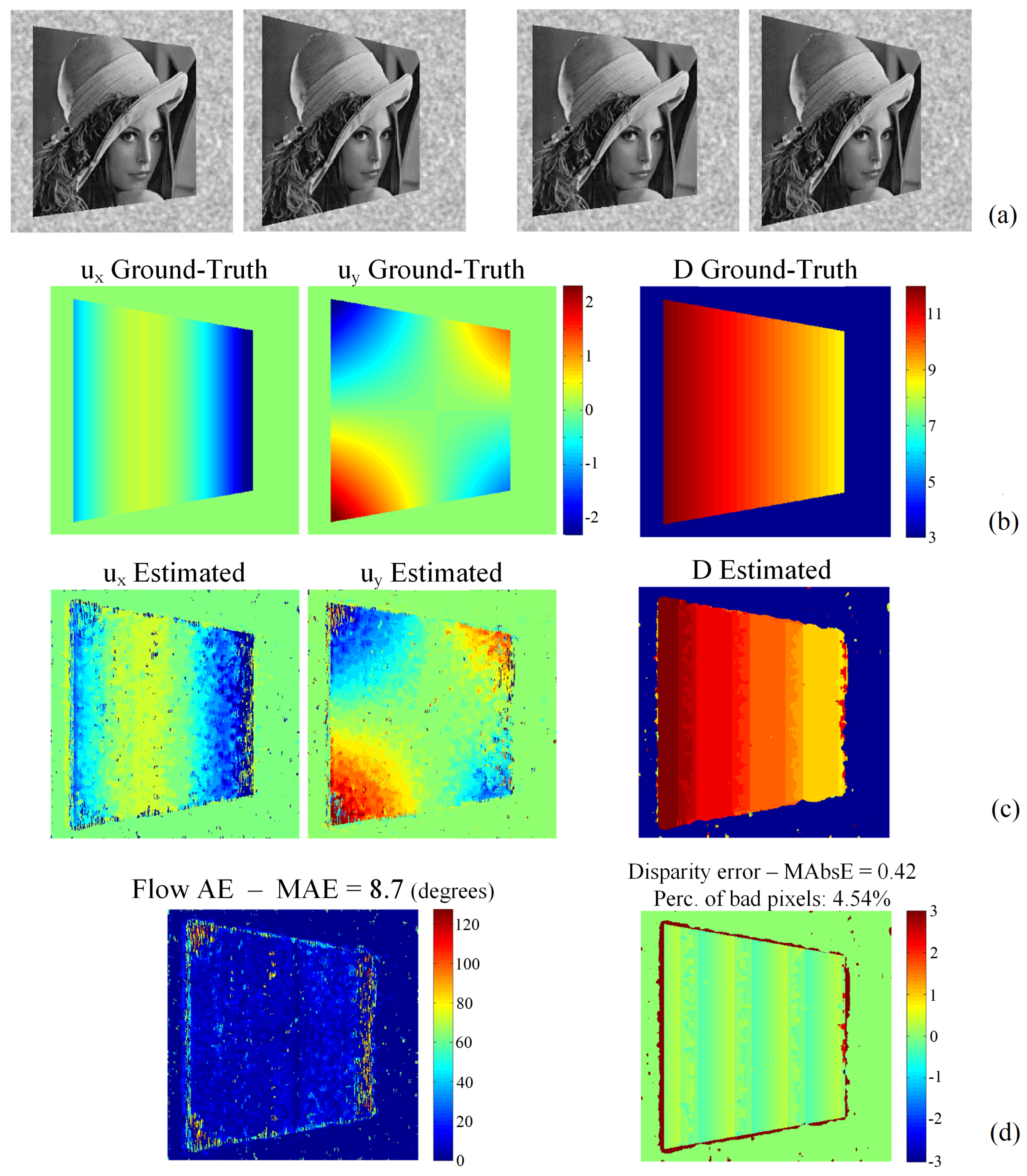
In this sequence, shown in Figure 9a, a textured 3D plane rotates constantly about the Y axis, introducing significant motion along the Z (depth) direction. The angle of the slanted plane is initially 15 and becomes equal to 25 in the last (sixth) frame. The GT motion field and disparity map are given in Figure 9b.
The proposed method was applied with filters of order and without employing the regularization and refinement steps. The results are given in Figure 9c,d. The MAE and disparity error remain at levels similar to the two previous sequences.
4.3. Experimental Results: Natural Sequences with Known Disparity GT
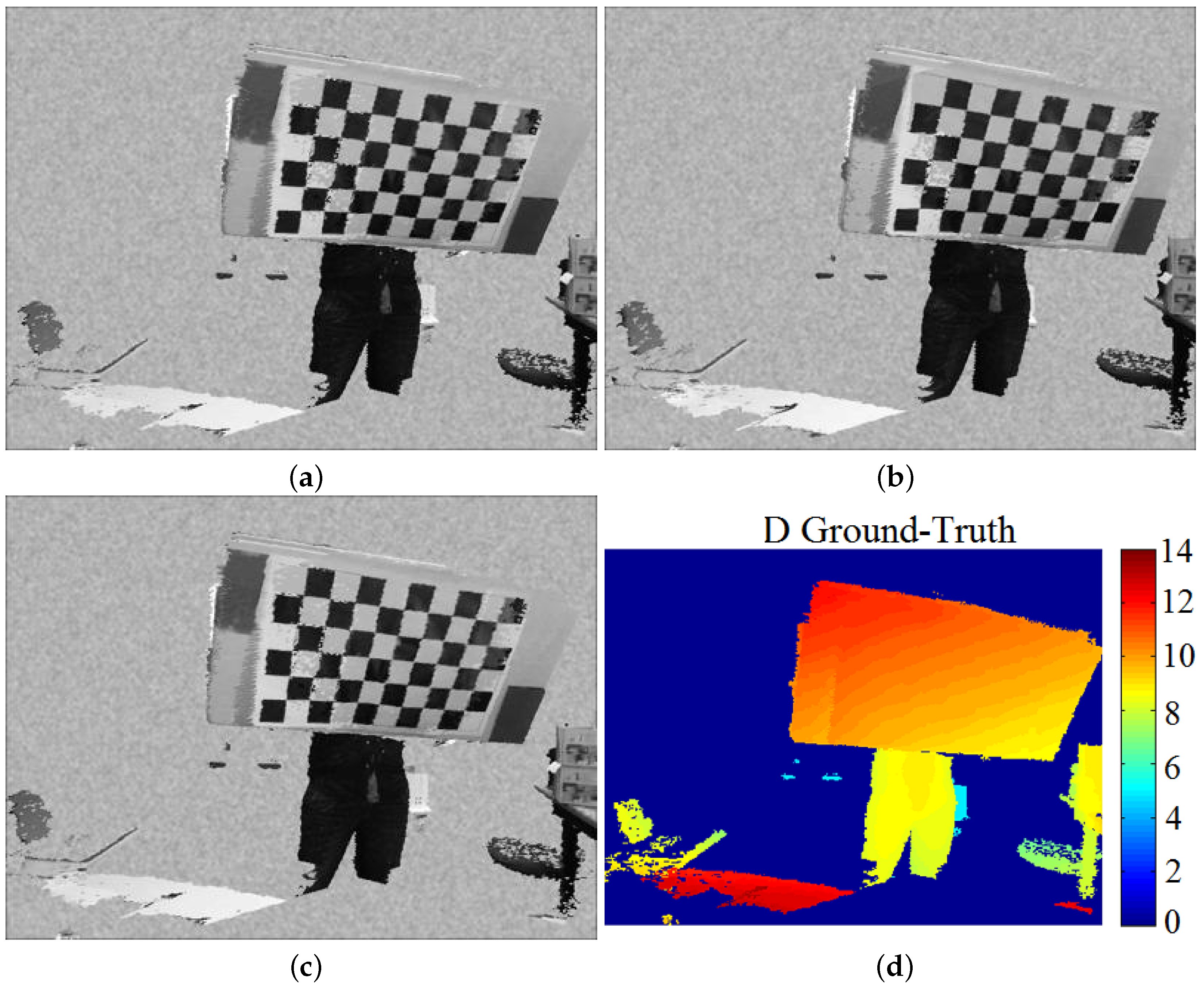
In this section, experimental results on natural stereo sequences are presented, for which however the disparity is known. The sequences were created using a custom-made tool, which lets one use 3D textured surface data (captured by Kinect sensors) to create multi-view image sequences: the 3D data are projected onto virtual OpenGL cameras (OpenGL FrameBuffers), the characteristics of which are known. Thus, disparity is also known.
The first sequence was generated from Kinect version2 RGB-Depth streams, whereas the second one was obtained from http://vcl.iti.gr/reconstructions. The background of the sequences is unknown. This “null” background is replaced by a smooth random pattern with zero disparity (see Figure 10). We note that (a) the sequences are noisy, in the sense that the 3D reconstructions contain geometrical and texture artefacts, especially at the object boundaries. Therefore, each view’s sequence is noisy, making the flow estimation task difficult. (b) On the other hand, the disparity estimation task is easier, since the stereo views of the same time-instance are “acquired” by virtual cameras and therefore are perfectly rectified.
4.3.1. “Dimitris-Chessboard” Sequence
This sequence, shown in Figure 10, includes a person that holds a chessboard pattern and moves towards right-backwards.
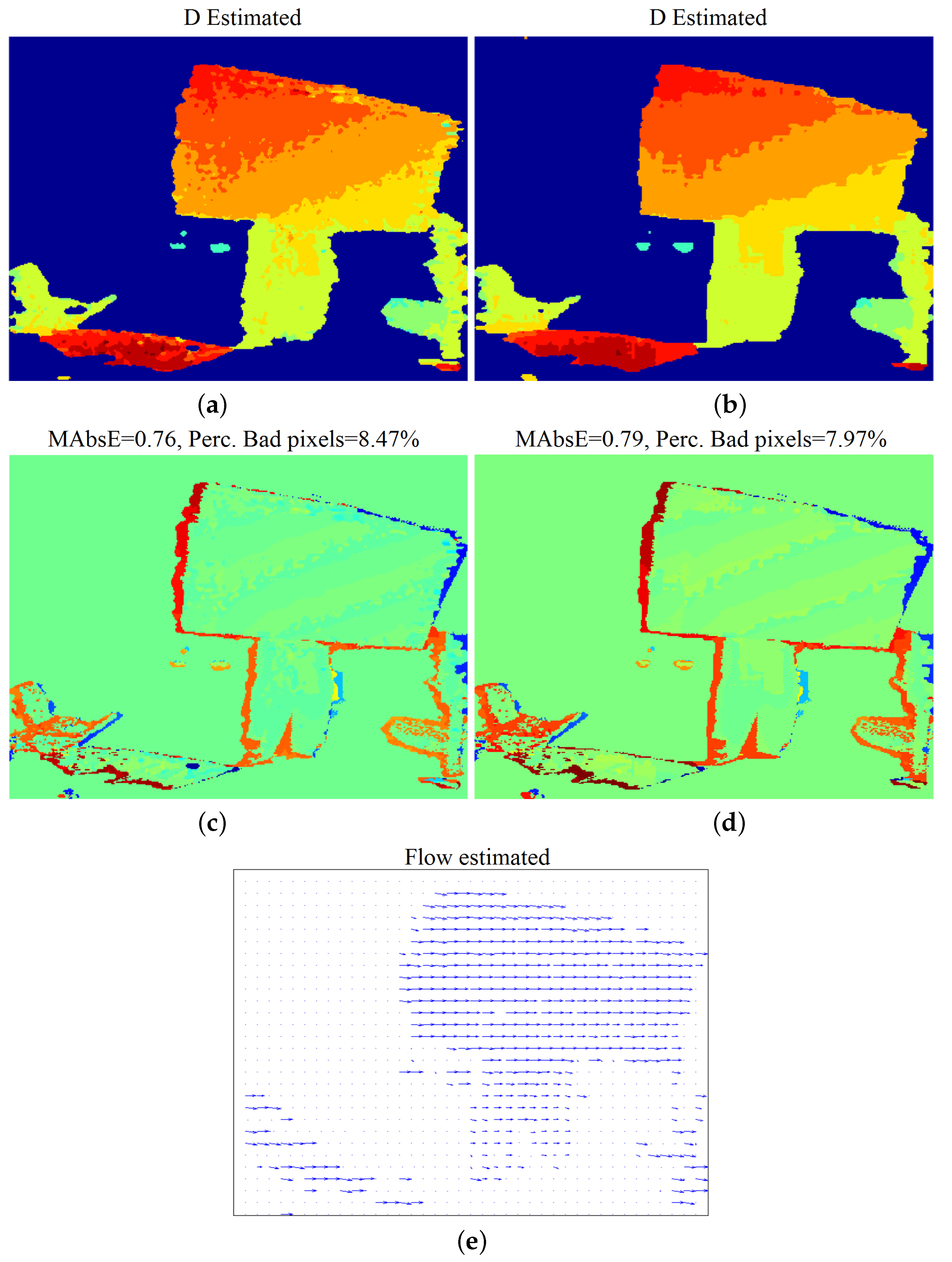
Results with respect to disparity estimation, without and with the application of Scan-Line Optimization (SO), are given in Figure 11a–d. The method manages to efficiently estimate disparity, even without SO optimization, despite the noisy input and the repeating “chessboard” pattern. The estimated map is less noisy, and the estimation error is slightly smaller when SO regularization is applied. The used parameters, as well as the computational time of the algorithmic parts, are given in Table 4.
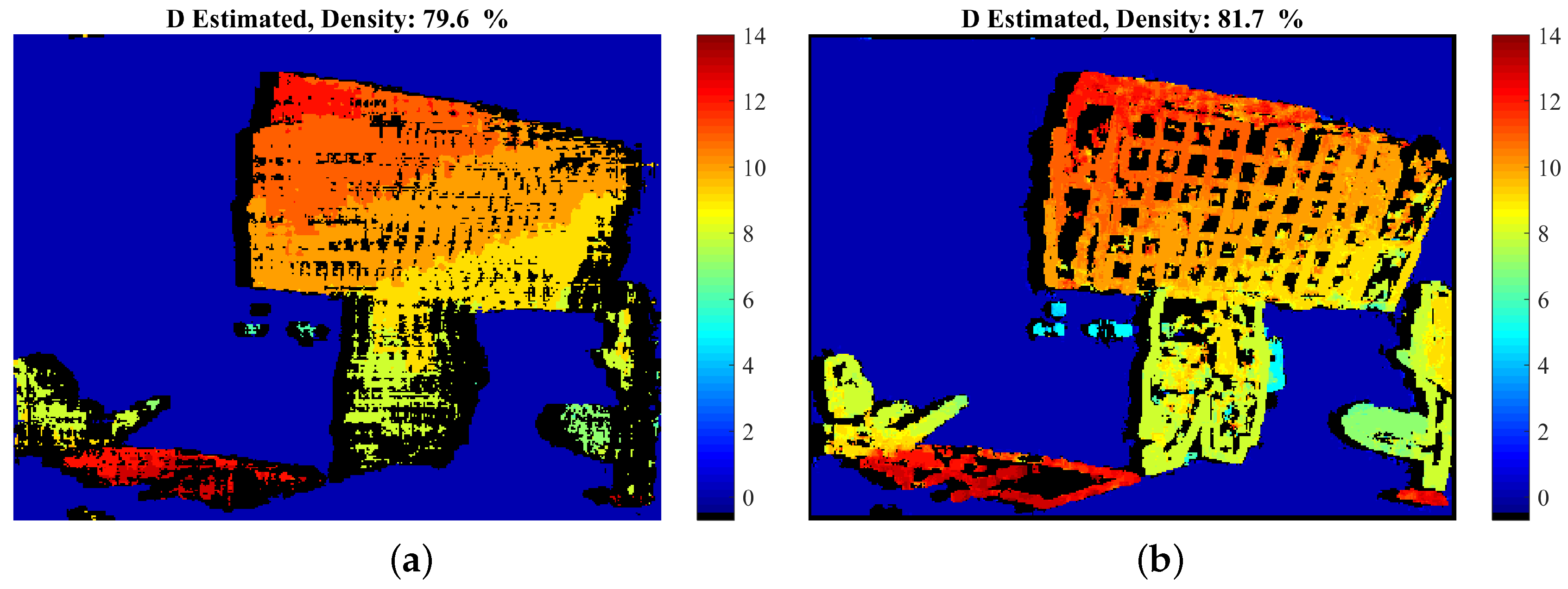
Table 5 and Figure 12 and Figure 13 provide comparative disparity estimation results. According to the table and Figure 13, the proposed method produces more accurate results at similar densities and similarly accurate results at 100% density.
Finally, the motion flow estimated by the proposed method (with SO) is given in Figure 11e. Although quantitative evaluation is not possible, one can say that the overall motion is adequately well estimated, even at the textureless lower-body part of the human. However, some very wrong estimates can be found, corresponding to static textureless and noisy captured regions, e.g., the white desk region at the bottom-left.
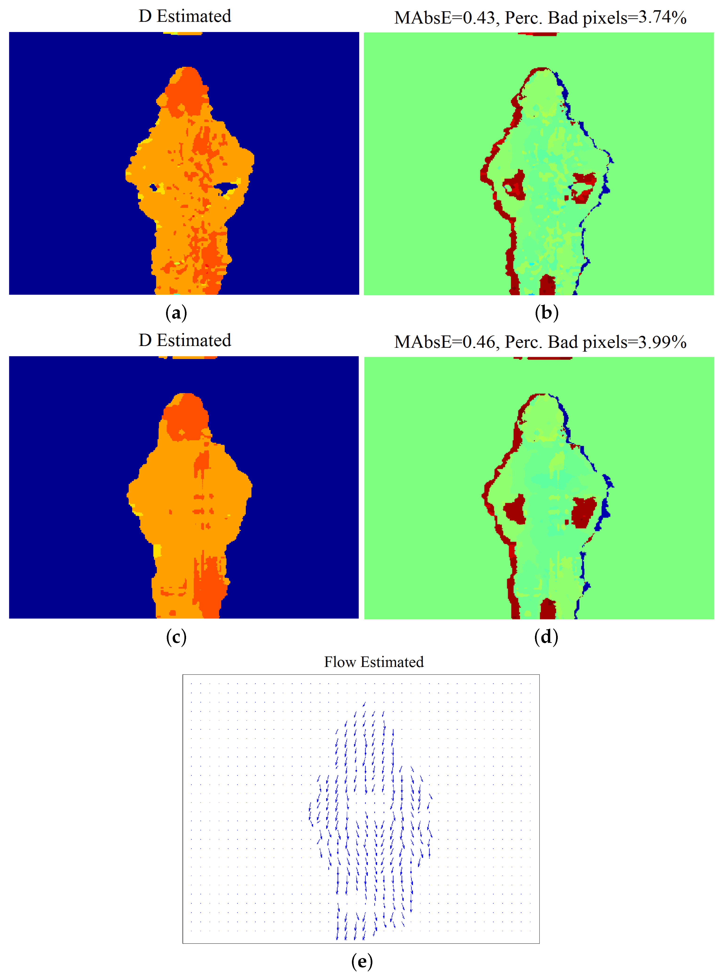
4.3.2. “Xenia” Sequence
In the “Xenia” sequence, depicted in Figure 14, Xenia bends her knees and moves downwards.
Exactly the same kind of results, as in the previous experiment, are given in Figure 15. The method efficiently estimates disparity, although the black clothes have poor texture and the sequence is noisy. In this experiment, however, the disparity estimates that Xenia’s silhouette boundaries are noisy, and the “edge-fattening” effect is more visible. This can be partially justified by the fact that the sequence was captured using Kinect1 devices, which provide more noisy measurements, and therefore, the 3D data were noisy at boundaries. Additionally, in this experiment, SO optimization seems to over-smooth the results, and thus, the corresponding errors are higher than those without SO.
With respect to the flow, Figure 15e shows that the flow estimation results are sensible and reflect the actual motion.
5. Discussion
In this work, a novel paradigm for frequency-domain or filter-based joint disparity and motion estimation was given. More specifically, from a theoretical point-of-view, the problem of joint disparity and motion estimation from stereo image sequences was initially studied in the spatiotemporal frequency domain. Guided by this study, a solution using steerable filters was then investigated. We extended the theory behind 3D steerable filters, and a novel steerable filter-based solution was developed. According to the authors’ knowledge, this work constitutes the first attempt towards joint depth and motion estimation based on frequency-domain and filter considerations. The ideas of this paper may constitute the basis for further theoretical and algorithmic developments.
We additionally extended the semi-global scan-line optimization (SO) method, originally developed for disparity estimation, in order to be used in our underlying problem. Combining the adapted SO method, as well as other relevant ideas from the disparity estimation literature, with the developed filter-based solution, an overall algorithm was formulated and successfully applied in the joint motion-disparity estimation problem. The algorithm was evaluated through a number of experimental results.
Acknowledgments
This work was supported by the F3SMEproject (PE6 3210), implemented within the framework of the Action “Supporting Postdoctoral Researchers” of the Operational Program “Education and Lifelong Learning”, and co-financed by the European Social Fund (ESF) and the Greek State.
Author Contributions
All three authors conceived the theoretical aspects of this work. Dimitrios Alexiadis and Nikolaos Mitianoudis designed the experiments; Dimitrios Alexiadis performed the experiments and analysed the data and the experimental results; All three authors wrote the paper.
Conflicts of Interest
The authors declare no conflict of interest. Additionally, the founding sponsors had no role in the design of the study; in the collection, analyses, or interpretation of data; in the writing of the manuscript, and in the decision to publish the results.
Abbreviations
The following abbreviations are used in this manuscript:
| DOG | Derivatives of Gaussian |
| MRF | Markov Random Field |
| NSSD | Normalized Sum of Squares Difference |
| GPU | Graphics Processing Unit |
| (F)FT | (Fast) Fourier Transform |
| SO | Scan-line Optimization |
| (M)AE | (Mean) Angular Error |
| WTA | Winner Take-it-All |
References
- Smolic, A. 3D video and free viewpoint video-From capture to display. Pattern Recognit. 2011, 44, 1958–1968. [Google Scholar] [CrossRef]
- Vedula, S.; Baker, S.; Rander, P.; Collins, R.; Kanade, T. Three-dimensional scene flow. IEEE Trans. Pattern Anal. Mach. Intell. 2005, 27, 475–480. [Google Scholar] [CrossRef] [PubMed]
- Ottonelli, S.; Spagnolo, P.; Mazzeo, P.L. Improved video segmentation with color and depth using a stereo camera. In Proceedings of the IEEE International Conference on Industrial Technology (ICIT), Cape Town, South Africa, 25–28 Febtuary 2013; pp. 1134–1139. [Google Scholar]
- Alexiadis, D.; Chatzitofis, A.; Zioulis, N.; Zoidi, O.; Louizis, G.; Zarpalas, D.; Daras, P. An integrated platform for live 3D human reconstruction and motion capturing. IEEE Trans. Circuits Syst. Video Technol. 2016, 27, 798–813. [Google Scholar] [CrossRef]
- Newcombe, R.; Fox, D.; Seitz, S. DynamicFusion: Reconstruction and Tracking of Non-rigid Scenes in Real-Time. In Proceedings of the IEEE Conference on Computer Vision and Pattern Recognition, Boston, MA, USA, 7–12 June 2015. [Google Scholar]
- Wang, Y.; Ostermann, J.; Zhang, Y. Video Processing and Communications; Prentice Hall: Upper Saddle River, NJ, USA, 2002. [Google Scholar]
- Scharstein, D.; Szeliski, R. A taxonomy and evaluation of dense two frame stereo correspondence algorithms. Int. J. Comput. Vis. 2002, 47, 7–42. [Google Scholar] [CrossRef]
- Barron, J.; Fleet, D.; Beauchemin, S. Performance of optical flow techniques. Int. J. Comput. Vis. 1994, 12, 43–77. [Google Scholar] [CrossRef]
- Black, M.J.; Anandan, P. The robust estimation of multiple motions: Parametric and piecewise-smooth flow fields. Comput. Vis. Image Underst. 1996, 63, 75–104. [Google Scholar] [CrossRef]
- Alexiadis, D.S.; Sergiadis, G.D. Narrow directional steerable filters in motion estimation. Comput. Vis. Image Underst. 2008, 110, 192–211. [Google Scholar] [CrossRef]
- Freeman, W.T.F.; Adelson, E.H. The design and use of steerable filters. IEEE Trans. Pattern Anal. Mach. Intell. 1991, 13, 891–906. [Google Scholar] [CrossRef]
- DeAngelis, C.; Ohzawa, I.; Freeman, R.D. Depth is encoded in the visual cortex by a specialized receptive field structure. Nature 1991, 352, 156–159. [Google Scholar] [CrossRef] [PubMed]
- Fleet, D.; Wagner, H.; Heeger, D. Neural Encoding of Binocular Disparity: Energy Models, Position Shifts and Phase Shifts. Vis. Res. 1996, 36, 1839–1857. [Google Scholar] [CrossRef]
- Adelson, E.H.; Bergen, J.R. Spatiotemporal energy models for the perception of motion. J. Opt. Soc. Am. A 1985, 2, 284–299. [Google Scholar] [CrossRef] [PubMed]
- Watson, A.B.; Ahumada, A.J. Model of human visual-motion sensing. J. Opt. Soc. Am. A 1985, 2, 322–341. [Google Scholar] [CrossRef] [PubMed]
- Qian, N. Computing Stereo Disparity and Motion with Known Binocular Cell Properties; Technical Report; MIT: Cambridge, MA, USA, 1993. [Google Scholar]
- Qian, N.; Andersen, R.A. A Physiological Model for Motion-stereo Integration and a Unified Explanation of Pulfrich-like Phenomena. Vis. Res. 1997, 37, 1683–1698. [Google Scholar] [CrossRef]
- Hirschmuller, H. Stereo processing by semiglobal matching and mutual information. IEEE Trans. Pattern Anal. Mach. Intell. 2008, 30, 328–341. [Google Scholar] [CrossRef] [PubMed]
- Cech, J.; Matas, J.; Perdoch, M. Efficient Sequential Correspondence Selection by Cosegmentation. IEEE Trans. Pattern Anal. Mach. Intell. 2010, 32, 1568–1581. [Google Scholar] [CrossRef] [PubMed]
- Kordelas, G.; Alexiadis, D.; Daras, P.; Izquierdo, E. Enhanced disparity estimation in stereo images. Image Vis. Comput. 2015, 35, 31–49. [Google Scholar] [CrossRef]
- Kordelas, G.; Alexiadis, D.; Daras, P.; Izquierdo, E. Content-based guided image filtering, weighted semi-global optimization and efficient disparity refinement for fast and accurate disparity estimation. IEEE Trans. Multimed. 2016, 18, 155–170. [Google Scholar] [CrossRef]
- Viola, P.; Wells, W.M. Alignment by maximization of mutual information. Int. J. Comput. Vis. 1997, 24, 137–154. [Google Scholar] [CrossRef]
- Vedaldi, A.; Soatto, S. Local features, all grown up. In Proceedings of the Computer Vision and Pattern Recognition (CVPR), New York, NY, USA, 17–22 June 2006. [Google Scholar]
- Huguet, F.; Devernay, F. A Variational Method for Scene Flow Estimation from Stereo Sequences. In Proceedings of the 11th IEEE ICCV conference, Rio de Janeiro, Brazil, 14–21 Octemner 2007; pp. 1–7. [Google Scholar]
- Valgaerts, L.; Bruhn, A.; Zimmer, H.; Weickert, J.; Stoll, C.; Theobalt, C. Joint Estimation of Motion, Structure and Geometry from Stereo Sequences. In Proceedings of the European Conference on Computer Vision, Heraklion, Greece, 5–11 September 2010. [Google Scholar]
- Cech, J.; Sanchez-Riera, J.; Horaud, R.P. Scene Flow Estimation by Growing Correspondence Seeds. In Proceedings of the IEEE Conference on Computer Vision and Pattern Recognition (CVPR), Colorado Springs, CO, USA, 20–25 June 2011; IEEE Computer Society Press: Los Alamitos, CA, USA, 2011; pp. 49–56. [Google Scholar]
- Liu, J.; Skerjanc, R. Stereo and motion correspondence in a sequence of stereo images. Signal Process. Image Commun. 1993, 5, 305–318. [Google Scholar] [CrossRef]
- Patras, I.; Alvertos, N.; Tziritasy, G. Joint Disparity and Motion Field Estimation in Stereoscopic Image Sequences; Technical Report TR-157; FORTH-ICS: Heraklion, Greece, 1995. [Google Scholar]
- Sizintsev, M.; Wildes, R.P. Spatiotemporal stereo and scene flow via stequel matching. IEEE Trans. Pattern Anal. Mach. Intell. 2012, 34, 1206–1219. [Google Scholar] [CrossRef] [PubMed]
- Sizintsev, M.; Wildes, R.P. Spacetime Stereo and 3D Flow via Binocular Spatiotemporal Orientation Analysis. IEEE Trans. Pattern Anal. Mach. Intell. 2014, 36, 2241–2254. [Google Scholar] [CrossRef] [PubMed]
- Isard, M.; MacCormick, J. Dense Motion and Disparity Estimation Via Loopy Belief Propagation. In Proceedings of the Computer Vision—ACCV 2006, Lecture Notes in Computer Science, Hyderabad, India, 13–16 January 2006; Volume 3852, pp. 32–41. [Google Scholar]
- Liu, F.; Philomin, V. Disparity Estimation in Stereo Sequences using Scene Flow. In Proceedings of the British Machine Vision Association, London, UK, 7–10 September 2009. [Google Scholar]
- Zitnick, C.L.; Kang, S.B. Stereo for image-based rendering using image over-segmentation. Int. J. Comput. Vis. 2007, 75, 49–65. [Google Scholar] [CrossRef]
- Zhang, Z. A flexible new technique for camera calibration. IEEE Trans. Pattern Anal. Mach. Intell. 2000, 22, 1330–1334. [Google Scholar] [CrossRef]
- Wedel, A.; Brox, T.; Vaudrey, T.; Rabe, C.; Franke, U.; Cremers, D. Stereoscopic Scene Flow Computation for 3D Motion Understanding. Int. J. Comput. Vis. 2011, 95, 29–51. [Google Scholar] [CrossRef]
- Yamaguchi, K.; McAllester, D.; Urtasun, R. Efficient Joint Segmentation, Occlusion Labeling, Stereo and Flow Estimation. In Proceedings of the European Conference on Computer Vision, Zurich, Switzerland, 6–12 September 2014. [Google Scholar]
- Taniai, T.; Sinha, S.N.; Sato, Y. Fast multi-frame stereo scene flow with motion segmentation. In Proceedings of the IEEE International Conference on Computer Vision and Pattern Recognition (CVPR), Honolulu, HI, USA, 21–26 July 2017. [Google Scholar]
- Walk, S.; Schindler, K.; Schiele, B. Disparity statistics for pedestrian detection: Combining appearance, motion and stereo. In Proceedings of the European Conference Computer Vision, Heraklion, Crete, 5–11 September 2010; pp. 182–195. [Google Scholar]
- Seguin, G.; Alahari, K.; Sivic, J.; Laptev, I. Pose Estimation and Segmentation of Multiple People in Stereoscopic Movies. IEEE Trans. Pattern Anal. Mach. Intell. 2015, 37, 1643–1655. [Google Scholar] [CrossRef] [PubMed]
- Simoncelli, E.P. Distributed Representation and Analysis of Visual Motion. Ph.D. Thesis, Department of Electrical Engineering and Computer Science, Massachusetts Institute of Technology, Cambridge, MA, USA, 1993. [Google Scholar]
- Terzopoulos, D. Regularization of inverse visual problems involving discontinuities. IEEE Trans. Pattern Anal. Mach. Intell. 1986, 8, 413–424. [Google Scholar] [CrossRef]
- Boykov, Y.; Veksler, O.; Zabih, R. Fast approximate energy minimization via graph cuts. IEEE Trans. Pattern Anal. Mach. Intell. 2001, 23, 1222–1239. [Google Scholar] [CrossRef]
- Hosni, A.; Rhemann, C.; Bleyer, M.; Rother, C.; Gelautz, M. Fast Cost-Volume Filtering for Visual Correspondence and Beyond. IEEE Trans. Pattern Anal. Mach. Intell. 2013, 35, 504–511. [Google Scholar] [CrossRef] [PubMed]
Figure 1.
Block diagram, summarizing the main steps of the algorithm.

Figure 2.
Simple artificial “Car-Tree” sequence: results with respect to the filters’ order N. The results were obtained by applying WTA directly to the initial cost volume : (a) first and last (sixth) frame of the left view and (b) ground-truth disparity map; (c) mean absolute disparity error and (d) percentage of bad pixels; (e) flow mean angular error; (f) computational time.

Figure 3.
Artificial “Futuristic White-Tower” sequence: (a) first and last (sixth) frame of the Left view; (b) ground-truth horizontal speed and disparity.
Figure 3.
Artificial “Futuristic White-Tower” sequence: (a) first and last (sixth) frame of the Left view; (b) ground-truth horizontal speed and disparity.


Figure 4.
Artificial “Futuristic White-Tower” sequence: estimation error results: (a) after only spatial aggregation (5 × 5); (b) after spatial aggregation (3 × 3) and scan-line optimization; (c) after the application of all steps.
Figure 4.
Artificial “Futuristic White-Tower” sequence: estimation error results: (a) after only spatial aggregation (5 × 5); (b) after spatial aggregation (3 × 3) and scan-line optimization; (c) after the application of all steps.

Figure 5.
Artificial “Futuristic White-Tower” sequence: estimation errors with respect to the step of the algorithm: (a) mean absolute disparity error; (b) percentage of bad pixels; (c) flow mean angular error, after the application of each algorithmic step.
Figure 5.
Artificial “Futuristic White-Tower” sequence: estimation errors with respect to the step of the algorithm: (a) mean absolute disparity error; (b) percentage of bad pixels; (c) flow mean angular error, after the application of each algorithmic step.

Figure 6.
Artificial “Futuristic White-Tower” sequence: estimation confidence map.
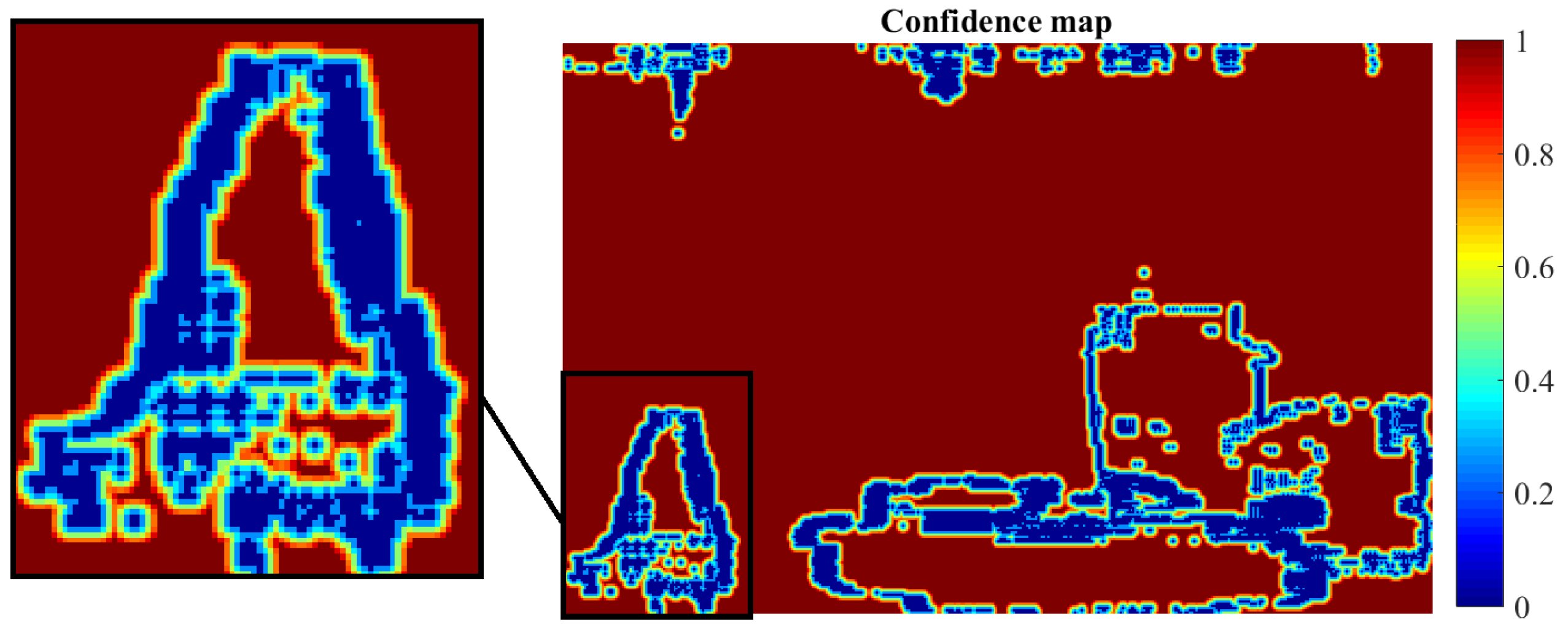
Figure 7.
Artificial “Futuristic White-Tower” sequence: comparative results: estimated disparity map of (a) the proposed method at density 86.5%, (b) GCSF [26] with density 84.4% and (c) MatCVTlbx-SemiG [26] with density 94.7%; estimated flow-field of (d) the proposed method and (e) GCSF [26]. For the corresponding estimation error, please refer to Table 2 and the diagrams of Figure 8.

Figure 8.
Artificial “Futuristic White-Tower” sequence: comparative results (a,b) with respect to disparity estimation and (c) with respect to flow estimation.
Figure 8.
Artificial “Futuristic White-Tower” sequence: comparative results (a,b) with respect to disparity estimation and (c) with respect to flow estimation.

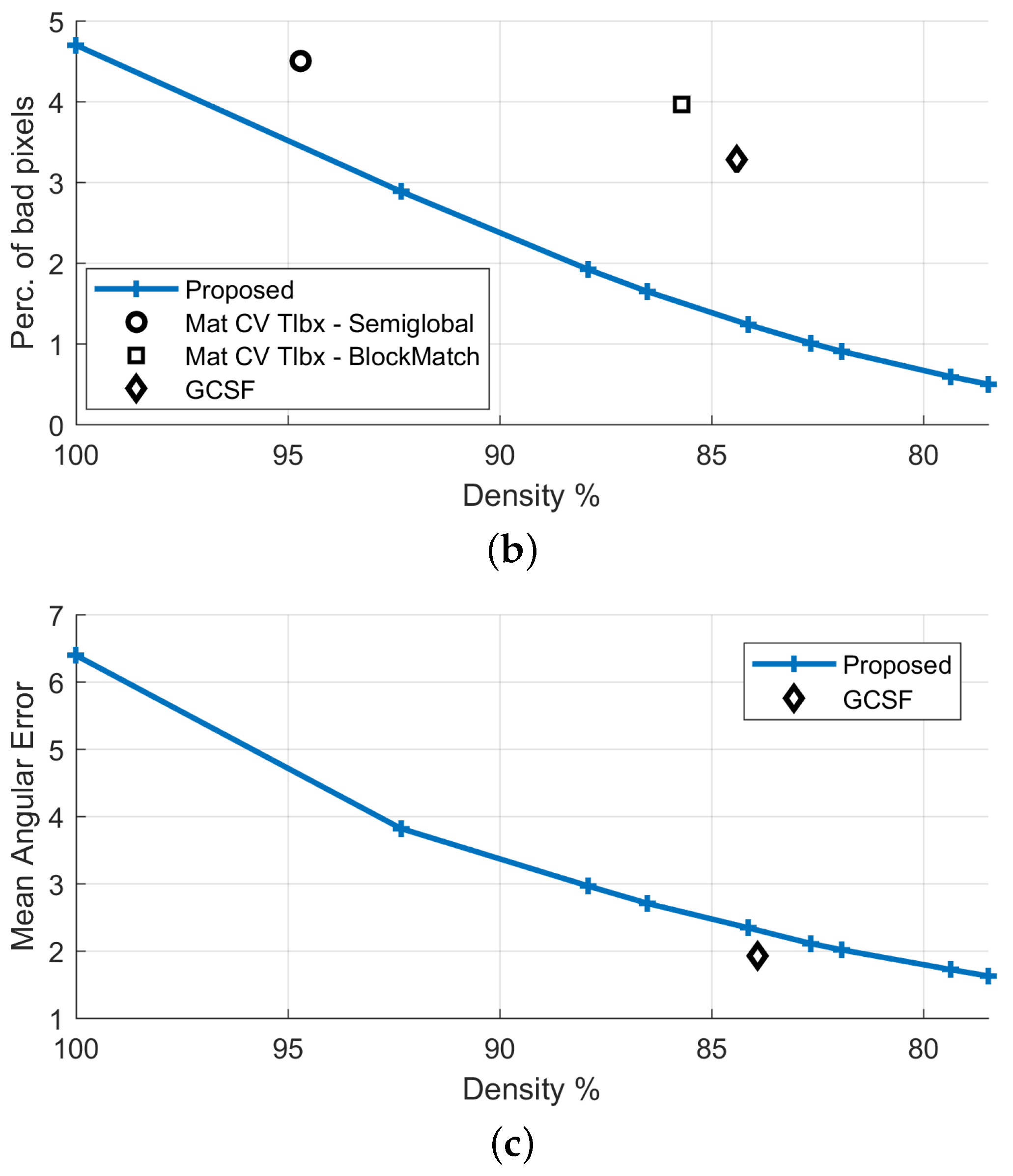
Figure 9.
Artificial “Rotating Lenna plane” sequence: (a) the first and last (sixth) frame of the left and right views; (b) the ground-truth flow and disparity; (c) the corresponding estimated flow and disparity map; (d) the flow angular error and disparity error.
Figure 9.
Artificial “Rotating Lenna plane” sequence: (a) the first and last (sixth) frame of the left and right views; (b) the ground-truth flow and disparity; (c) the corresponding estimated flow and disparity map; (d) the flow angular error and disparity error.

Figure 10.
“Dimitris-Chessboard” sequence: (a,b) first and last (sixth) frame of the left view; (c) first frame of the right view; (d) ground-truth of disparity.
Figure 10.
“Dimitris-Chessboard” sequence: (a,b) first and last (sixth) frame of the left view; (c) first frame of the right view; (d) ground-truth of disparity.

Figure 11.
“Dimitris-Chessboard” sequence: experimental results: estimated disparity map (a) before and (b) after the application of SO; (c,d) the corresponding estimation error results; (e) estimated flow field after the application of SO.
Figure 11.
“Dimitris-Chessboard” sequence: experimental results: estimated disparity map (a) before and (b) after the application of SO; (c,d) the corresponding estimation error results; (e) estimated flow field after the application of SO.

Figure 12.
Natural “Dimitris-Chessboard” sequence: comparative results: Estimated disparity map of (a) the proposed method at density 79.6% and (b) GCSF [18] with density 81.7%. For the corresponding estimation error, please refer to Table 5 and the diagrams of Figure 13.

Figure 13.
Natural “Dimitris-Chessboard” sequence: comparative results with respect to disparity estimation.
Figure 13.
Natural “Dimitris-Chessboard” sequence: comparative results with respect to disparity estimation.
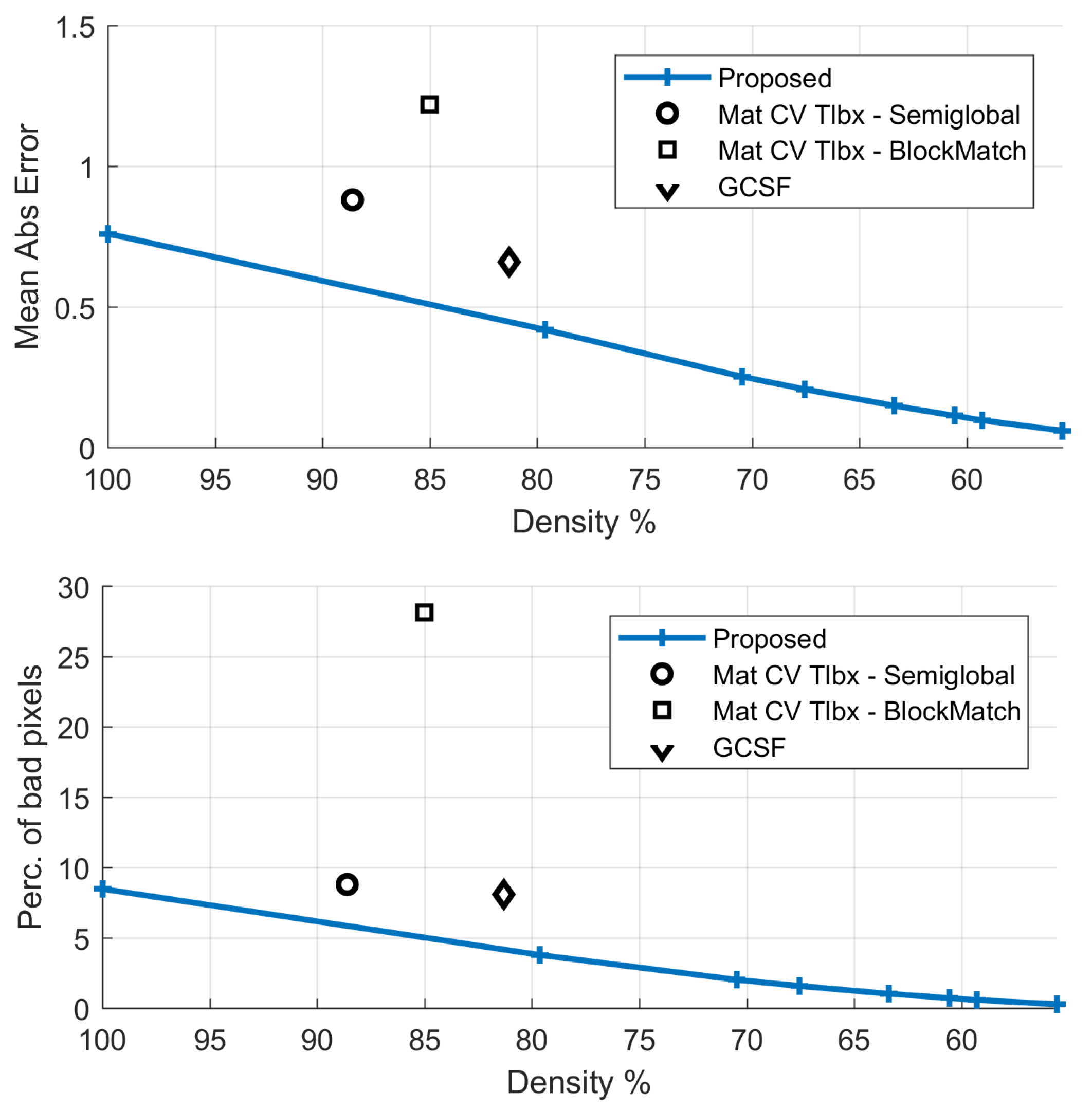
Figure 14.
“Xenia” sequence: (a,b) first and last (sixth) frame of the left view; (c) first frame of the right view; (d) ground-truth of disparity.
Figure 14.
“Xenia” sequence: (a,b) first and last (sixth) frame of the left view; (c) first frame of the right view; (d) ground-truth of disparity.
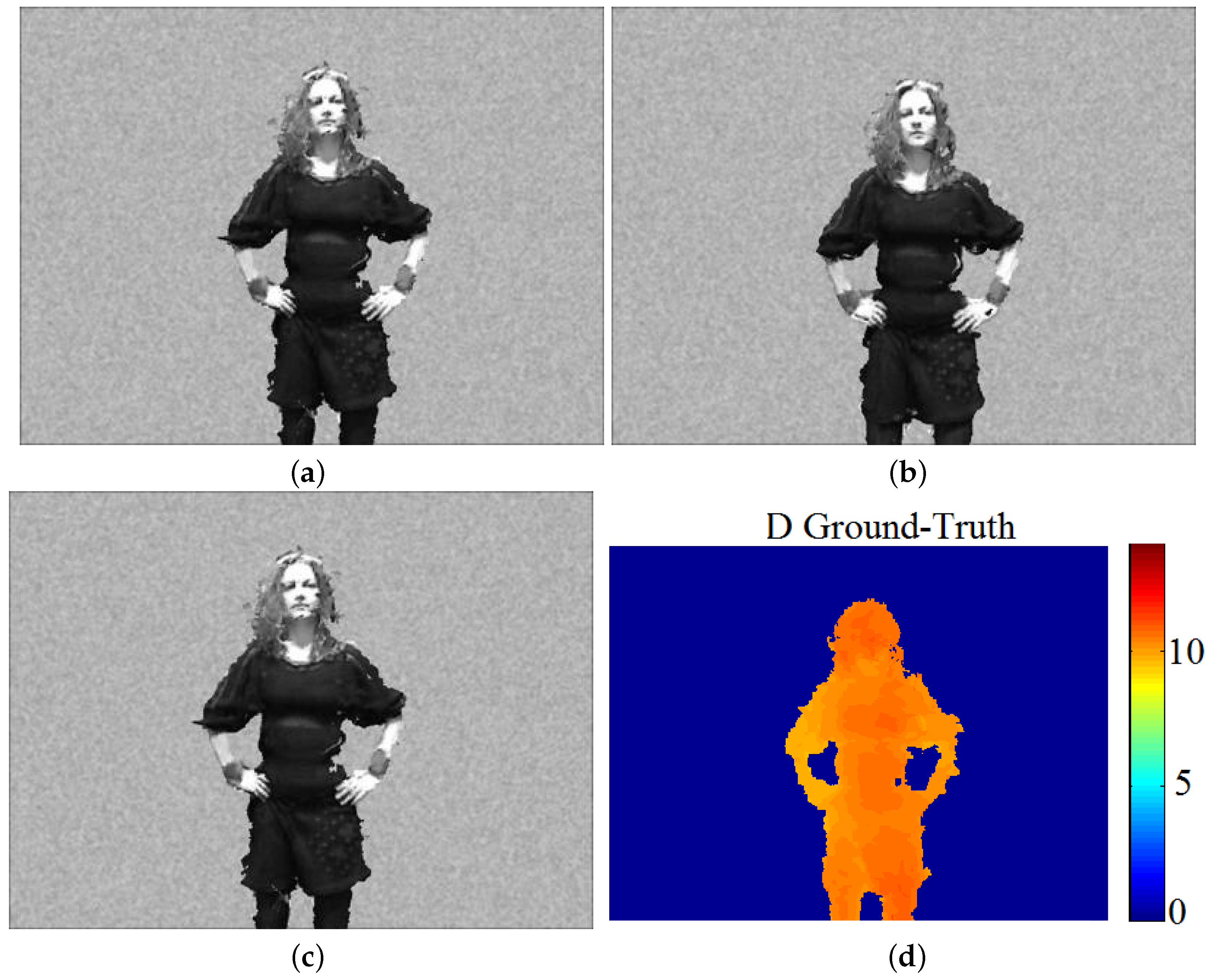
Figure 15.
“Xenia” sequence: experimental results: estimated disparity map (a) before and (b) after the application of SO; (c,d) the corresponding estimation error results; (e) estimated flow field after the application of SO.
Figure 15.
“Xenia” sequence: experimental results: estimated disparity map (a) before and (b) after the application of SO; (c,d) the corresponding estimation error results; (e) estimated flow field after the application of SO.

Figure 16.
Natural “Xenia” sequence: Comparative results with respect to disparity estimation.


Table 1.
Parameters and computational time (CPU vs. GPU) for the “Futuristic White-Tower” sequence.
| Sequence: “Futur.WT” | Resolution: | No. of Frames: 6 | ||
|---|---|---|---|---|
| Parameters | ||||
| Filters | Candidate | Candidate | ||
| Order | Velocities | Disparities | ||
| Algorithmic Part | Computational Time (ms) | GPU | ||
| CPU Impl. | GPU Impl. | Speed-Up | ||
| Init. cost volume calculation | 27,156 | 7423 | 3.65:1 | |
| Scan-line optimization | 433,794 | 103,899 | 4.18:1 | |
Table 2.
Comparative results for the “Futuristic White-Tower” sequence. GCSF, Growing Correspondence Seeds for scene Flow; FD, Full Density.
Table 2.
Comparative results for the “Futuristic White-Tower” sequence. GCSF, Growing Correspondence Seeds for scene Flow; FD, Full Density.
| Method | Dispar.Density | Mean AbsError | Perc.Bad Pixels | Flow Density | Mean Angul.Error |
|---|---|---|---|---|---|
| Proposed (FD) | 100% | 0.31 | 4.78% | 100% | 5.83 |
| Proposed | 86.5% | 0.10 | 1.65% | 86.5% | 2.71 |
| GCSF [26] | 84.4% | 0.17 | 3.28% | 83.9% | 1.93 |
| MatCVTlbx-SemiG [18] | 94.7% | 0.33 | 4.50% | - | - |
| MatCVTlbx-Block | 85.7% | 0.27 | 3.96% | - | - |
Table 3.
Comparative results for the “Rotating Lenna plane” sequence.
| Method | Dispar.Density | Mean Abs Error | Perc. Bad Pixels | Flow Density | Mean Angul. Error |
|---|---|---|---|---|---|
| Proposed-Step 2 (FD) | 100% | 0.42 | 4.54% | 100% | 8.70 |
| GCSF [26] | 89.1% | 0.31 | 3.71% | 87.5% | 10.18 |
| MatCVTlbx-SemiG [18] | 93.9% | 0.38 | 5.38% | - | - |
| MatCVTlbx-Block | 87.5% | 0.47 | 6.69% | - | - |
Table 4.
Parameters and computational time (CPU vs. GPU) for the “Dimitris-Chessboard” sequence.
| Sequence: “Dimitris” | Resolution: | No. of Frames: 6 | ||
|---|---|---|---|---|
| Parameters | ||||
| Filters | Candidate | Candidate | ||
| Order | Velocities | Disparities | ||
| Algorithmic Part | Computational Time (ms) | GPU | ||
| CPU Impl. | GPU Impl. | Speed-Up | ||
| Init. cost volume calculation | 30,283 | 7564 | 4.00:1 | |
| Scan-line optimization | 405,071 | 86,295 | 4.69:1 | |
© 2018 by the authors. Licensee MDPI, Basel, Switzerland. This article is an open access article distributed under the terms and conditions of the Creative Commons Attribution (CC BY) license (http://creativecommons.org/licenses/by/4.0/).
Share and Cite
MDPI and ACS Style
Alexiadis, D.; Mitianoudis, N.; Stathaki, T. Frequency-Domain Joint Motion and Disparity Estimation Using Steerable Filters. Inventions 2018, 3, 12. https://doi.org/10.3390/inventions3010012
AMA Style
Alexiadis D, Mitianoudis N, Stathaki T. Frequency-Domain Joint Motion and Disparity Estimation Using Steerable Filters. Inventions. 2018; 3(1):12. https://doi.org/10.3390/inventions3010012
Chicago/Turabian StyleAlexiadis, Dimitrios, Nikolaos Mitianoudis, and Tania Stathaki. 2018. "Frequency-Domain Joint Motion and Disparity Estimation Using Steerable Filters" Inventions 3, no. 1: 12. https://doi.org/10.3390/inventions3010012