Numerical Study on Single Flowing Liquid and Supercritical CO2 Drop in Microchannel: Thin Film, Flow Fields, and Interfacial Profile


1
Department of Mechanical and Mechatronics Engineering, University of Waterloo, Waterloo, ON N2L 1W2, Canada
2
School of Mechanical Engineering and Automation, Harbin Institute of Technology, Shenzhen 518055, China
*
Author to whom correspondence should be addressed.
Inventions 2018, 3(2), 35; https://doi.org/10.3390/inventions3020035
Submission received: 10 April 2018
/
Revised: 16 May 2018
/
Accepted: 29 May 2018
/
Published: 1 June 2018
(This article belongs to the Special Issue Microfluidics and Nanofluidics)
Abstract
:Taylor segments, as a common feature in two- or multi-phase microflows, are a strong flow pattern candidate for applications when enhanced heat or mass transfer is particularly considered. A thin film that separates these segments from touching the solid channel and the flow fields near and inside the segment are two key factors that influence (either restricting or improving) the performance of heat and mass transfer. In this numerical study, a computational fluid dynamics (CFD) method and dense carbon dioxide (CO2) and water are applied and used as a fluid pair, respectively. One single flowing liquid or supercritical CO2 drop enclosed by water is traced in fixed frames of a long straight microchannel. The thin film, flow fields near and within single CO2 drop, and interfacial distributions of CO2 subjected to diffusion and local convections are focused on and discussed. The computed thin film is generally characterized by a thickness of 1.3~2.2% of the channel width (150 µm). Flow vortexes are formed within the hydrodynamic capsular drop. The interfacial distribution profile of CO2 drop is controlled by local convections near the interface and the interphase diffusion, the extent of which is subject to the drop size and drop speed as well.

1. Introduction
Fluid segments (e.g., bubbles, droplets) in microfluidic devices are generally characterized by large surface-to-volume ratios and short transfer distances which enhance heat and mass transfer. As two-phase flows involving gas–liquid and liquid–liquid are considered in a microscale device, they mostly feature an interface that separates one phase from the other. Thus, interfacial effects (e.g., interfacial tension, contact angle) start to dominate flow behaviors (e.g., flow regimes) and topological changes (e.g., breakup or coalescence) relative to other factors, such as inertial and gravitational forces. Among all possible flow regimes, slug flows (which may also be called “segmented flows” or “Taylor flows”) have become one of the most studied regimes in experimental and numerical studies concerning flow patterns, flow fields in slugs, slug profiles, thin film thicknesses and effects, etc. Compared with experimental methods in general, numerical simulations have not been widely employed to study two-phase microflows, which is mainly due to the three-dimensional nature of the flow which results in high cost in computation power and time and limited numerical methods developed for two-phase flows. However, rapid developments in computational methods and equipment have promoted the applications of numerical methods in two-phase microfluidic simulations, especially in those interface-involved-and-resolved ones over the last two decades [1,2,3,4,5].
Interface resolving is required in numerical simulations of slug flows in which the interface is often unsteady and deformable. Thus, a numerical method for application must be able to resolve the interface evolution spatially and temporally, such as the one among moving-grid and front-tracking in Lagrangian types or volume-of-fluid (VOF) and level-set (LS) in Eulerian types [5]. Moreover, based on a continuum assumption of the discussed matter where the Knudsen number (Kn = λ/L, λ and L indicate a mean free path of molecules and a characteristic length, respectively) is extremely small (below 0.001), general governing equations (i.e., continuity, momentum, and energy equation) of transport phenomena are applicable to both phases as well as the interface at a micro length scale (i.e., tens to hundreds of microns) [4]. In the scope of continuum assumption, the interface can be deemed with either a zero thickness (i.e., sharp interface) or a non-zero thickness. For the former scenario, there exist methods such as interface reconstruction VOF, LS, and front-tracking; and for the latter scenario, methods including color function VOF, conservation LS, and phase-field can be considered. Detailed descriptions of the methods are referred to a review by Wörner [4].
Most of the above methods have been applied in numerical studies for slug flows in microchannels (mostly circular cross-sectional). For example, Taha and Cui [6] used piece linear interface calculation (PLIC) (for interface reconstruction) based VOF for probing the hydrodynamics of long gas bubbles in capillaries. A similar strategy combined with a continuum surface force (CSF) model for modeling surface tension effects was applied in simulating Taylor flows in horizontal microchannels [3]. Fukagata et al. [7] numerically studied Taylor flows with a focus on heat transfer in a two-dimensional and axisymmetric tube using a LS method. A phase-field method was applied by He et al. [8] in revealing the bubble shape, superficial velocities of gas and liquid in a two-dimensional and axisymmetric channel for gas–liquid two-phase flows. Another popular method, lattice Boltzmann method was used by Yu et al. [9] in the numerical part of their study of gas–liquid flow in rectangular microchannels. However, there are still less studies dedicated to the slug flow in non-circular channels, such as rectangular or even triangular ones [1,4,10]. The mass transfer across the interface in slug flows is regarded one important mechanism of liquid extraction and phase separation [11]. In fact, numerical methods can be applied to give an insight into the interphase mass transfer with or without reactions. Schuster et al. [12] investigated gas–liquid two-phase flows in mini/micro scale channels and the interphase mass transport in both a falling film and a membrane reactor with a finite element method based software package, FEMLAB (later known as COMSOL). Raimondi et al. [13] implemented direct two-dimensional simulations (self-developed codes called JADIM) in studying the mass transfer of liquid–liquid slug flows in a square microchannel subjected to various flow velocities and channel geometries. Shao et al. [14] used COMSOL to simulate chemical CO2 adsorption to an alkaline solution in a gas–liquid Taylor flow in capillaries, in which the physical and chemical absorption at the interface were analyzed and compared in terms of absorption fraction and volumetric mass transfer coefficient. PLIC based VOF methods were used by Onea et al. [15] and Kececi et al. [16] in their three-dimensional simulations on mass transfer of upward and downward gas–liquid Taylor flows in rectangular microchannels.
Liquid and supercritical (sc-)CO2 are very possibly the two dense states of fluid CO2 when it is injected and stored in deep underground geoformations or oceanic seabed. Due to the presence of in situ resident water, the CO2 is likely to form a partially miscible fluid pair with it. This fluid pair has attracted increasing interests in the microfluidics research community [17], with particular interests in interphase mass transfer resulted size changes of the Taylor-type CO2 segments [18]. Despite some experimental work on gaseous CO2, studies related to dense CO2 are very rare. Generally, it is a technical challenge to experimentally probe dense CO2 interacting with water within microscale geometries due to extreme operation conditions. However, numerical simulations can be a useful method for such studies. In addition, it is scientifically meaningful to do so accounting for the very distinct physical properties (e.g., density, viscosity, diffusivity) of dense CO2, in particular scCO2, than gaseous CO2 that may lead to very different flow behavior or interphase mass transfer performance. Usually, such numerical studies can be partly carried out by using a few dimensionless numbers, such as capillary numbers, Reynolds numbers, and Weber numbers, etc.
Here, we report a numerical study of one single flowing liquid and scCO2 drop in a long straight rectangular microchannel analogous to that in our previous experimental studies [18,19]. We focus on understanding CO2 drop profile, thin water film, flow fields near and within CO2 drops, and interfacial profile of CO2 drops subjected to diffusion and local convections at the interface. In Section 2, fundamentals of the numerical simulations including general assumptions and governing equations are introduced. The numerical problem are formulated and the solution method are detailed in Section 2 as well. In Section 3, results are shown and discussed. Discussions on limitations of our numerical simulations are given in Section 4. A conclusion is provided in Section 5.
2. Numerical Methodology
2.1. General Assumptions
Liquid and supercritical CO2 are used as a drop phase, respectively, in this numerical study. The CO2 drop flows at a specifically designated superficial speed (see Table 1). DI (de-ionized) water is a continuously flowing carrier liquid in the microchannel. All fluids here are assumed incompressible and Newtonian and are characterized by constant densities and viscosities for a given set of temperature and pressure. The problem is under an isothermal condition and the interfacial tension between CO2 and water is constant as imported (thus, Marangoni effects on the interface are not considered). Moreover, the interface between the CO2 drop and water is a sharp interface, i.e., an interface with a zero thickness. In addition, gravitational forces are not considered, which is rational given that the range of the Bond number [Bo: (1.65~4.5) × 10−3] in the problem. Besides, the wettability of the channel wall is assumed uniform and steady, and constant contact angles are implemented.
2.2. Governing Equations
CFD software FLUENT (version 17.0, Ansys Inc., Canonsburg, PA, USA) is used for simulations here. A finite volume based method is used by FLUENT to discretize the governing equations. In order to resolve the interface, the volume-of-fluid (VOF) method is based on a fraction function of “α” in each cell which lies between 0 and 1. If α = 1, it indicates that the cell is full with one phase of interest; while α = 0 means that the cell is full of the other phase. α falling in between 0 and 1 indicates that the fluids co-exist in the cell. The interface resolving is achieved based on a volume fraction equation (also called advection equation) of the main phase, as shown below.
Volume fraction equation:
in which t is time and is the velocity vector of the fluid. The volume fraction of the other phase is not solved, instead can be obtained according to
Based on assumptions of conditions such as Newtonian and incompressible, the continuity and the momentum equations are applicable to either or both of the phases. Instead of an overall continuity equation, a convection-diffusion of the primary phase “i” is introduced here and written as
where ρi is the density of phase i, is a diffusion flux from phase i to the other across the interface, and Ri is a net production rate of phase i (or called specie “i”) due to chemical reactions. In this work, the chemical reaction is not considered, thus Ri is zero in Equation (3). In addition, is generally specified by a sum of mass diffusion and thermal diffusion, but here the thermal (or called Soret) diffusion is not considered according to an isothermal assumption. Therefore, can be specified under a dilute approximation (i.e., mass fraction of specie “i” in the mixture region is much smaller than 1) as
in which Dim is the mass diffusivity of specie “i” in the mixture region. Equations (3) and (4) are applicable to the other phase as well since two phases are involved here. The sum should result in a common overall continuity equation, as shown below.
Overall continuity equation:
in which ρ is the bulk density. Besides, a single momentum equation can be solved throughout the entire domain and the solved velocity field is shared among both phases. The momentum equation is detailed below.
Momentum equation:
where P is the pressure, µ is the bulk dynamic viscosity, is the gravitational acceleration, and is the volumetric interfacial force per unit area. On the right hand side of Equation (6), the term is a viscous stress tensor which may be designated as “τ”.
2.2.1. Surface Tension Model
A surface tension model in FLUENT, namely, continuum surface force (CSF) treats surface tension as a source term in the momentum equation [20], as shown in Equation (6). At the interface between the two phases, pressure difference across the interface is correlated to surface tension according to the Young–Laplace equation by
in which σ is the surface tension, is the capillary pressure induced by the surface tension, R1 and R2 are two principal radii of the interface, and indicates the curvature of the interface. If is a surface normal at the interface, then it can be expressed as the gradient of the volume fraction () of the “i” phase as follows
Thus, the unit normal can be obtained, . Curvature is defined as the divergence of the unit normal, , which can be expressed as
in which is a Laplace operator. When the two phases appear in the same cell, a volume force will occur which can be written based on Equations (7)–(9) as
where is a Dirac distribution correlated with the interface [4,10]. Note that Equation (10) is only active in the interfacial region.
2.2.2. Fluid Property Treatment
Shown in Equations (5) and (6), bulk density ρ and bulk dynamic viscosity µ are generally used in the continuity and the momentum equation, respectively. When the cell is purely filled by one phase “i”, the bulk density and viscosity are exactly the phase density and viscosity. However, in the interfacial region where the cell may be filled by both phases, the bulk density ρ and the bulk viscosity µ need to be weighted, e.g., by the volume fraction α and the mass fraction, respectively
and
where and are the pure phase density and viscosity, respectively.
2.3. Problem Formulation
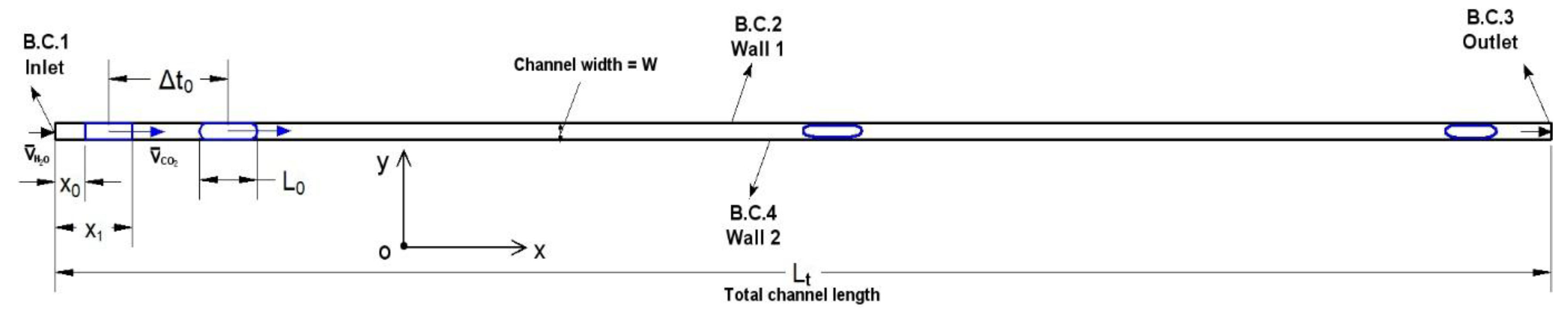
In this work, a two-dimensional (2D) computational domain for the flow field in a Cartesian coordinate system is considered, as shown in Figure 1. This domain falls into the group of a fixed frame type according to Talimi et al. [1], thus long computation time is expected. The straight channel is horizontally oriented. A constant flow of water in terms of mean velocity () starts at the inlet (boundary condition B.C. 1) on the left end, and the fluids will flow out of the channel eventually at the outlet on the right end (an outflow boundary, B.C. 3). The boundary condition is fulfilled by the other two, i.e., B.C. 2 and B.C. 4 which are no slip and rigid walls.
Note that none of the common geometries (e.g., T-junction, flow-focusing device) are applied for producing droplets in the simulation here. Alternatively, the to-be-investigated liquid CO2 or scCO2 drop is formed by marking a specific region located closely to the inlet as an initialized CO2 drop. The marked region (a rectangular cuboid shape) is 0.2 mm and 0.3 mm from its left boundary to the inlet for liquid CO2 drops and scCO2 drops, respectively, as shown by x0 in Figure 1. The assigned x0 should be longer than the entrance distance (related to the Reynolds number, Re = , which is generally 1.6–2.3 × 10⁻¹¹) of the channel for water flow to be fully developed. Thus, the entrance distance is almost zero in this problem. Furthermore, the right-hand side boundary is x1 to the inlet. The difference (x1 − x0) exactly defines the length of the initialized CO2 drop. In addition to x-dimension, the width of the marked region on y-dimension is equivalent to the channel width. Nevertheless, the initialized CO2 drop takes some computation time to develop into a realistic cylindrical shaped drop (with a length L0). The computation time is indicated by Δt0. Generally, Δt0 is a small quantity (<10%) compared with the subsequent overall flowing time of the CO2 drop in the straight channel. After a certain computation time as the vertex of the front meniscus of the CO2 drop reaches the outlet of the channel, the simulation is considered finished and will then be manually terminated.
2.4. Meshing
A VOF method based on finite volume discretization is used to solve Equations (1), (5) and (6) on a 2D staggered Cartesian mesh. The computational domain is meshed into 2999 × 119 (on x-axis and y-axis, respectively) quadrilateral cells. A total of 356,881 cells result in 716,880 faces and 360,000 nodes as well.
In the entire domain, each cell has a uniform length of 5 µm and is of a width (in the y-dimension) of ~1.3 µm in the bulk central region. Moreover, the grid is refined by using further reduced cell widths (approaching 0.1 µm) near the wall region (its overall width is 3 µm or so which equals to 2% W) in order to compute out the thin film that separates the CO2 drop from touching the channel wall. Note that the meshing is axisymmetric, thus the meshing is the same at the other channel wall (Wall 2 in Figure 1). This mesh structure was the result of grid independence testing. The meshing method and the grid resolutions are maintained as fixed over the entire simulation work.
2.5. Simulation Cases and Material Properties
In this work, six cases in total are investigated, which are designated by the specific ratio of the flow rate of CO2 and that of water as applied in our previous experimental work [18,19]. Table 1 lists detailed information of all the six simulation cases, including corresponding QCO2/QH2O, the distance of the initialized drop at its left boundary to the channel inlet (x0), the length of the initialized CO2 drop (x1 − x0), and the superficial flow velocities of the water and the initialized drops. Note that (x1 − x0) for each case is assigned in accordance with the length of generated CO2 drop under the corresponding QCO2/QH2O. Furthermore, superficial flow velocity and of the continuous phase (water) and the CO2 drop, as initial conditions, correspond to the experimentally measured drop speeds. is equivalent to according to a single-field (or called “shared-field”) formulation in which the flow field is shared by the co-current phases as shown by the momentum equation (i.e., Equation (6)).
For the simulation cases listed in Table 1, material properties of the applied DI water, the liquid CO2 and the scCO2 are referred to those at the pressure and temperature that have been used [18,19]. The material properties—including density, viscosity, mass diffusivity, interfacial tension, and contact angle—are listed in Table 2.
The temperatures for liquid CO2 and scCO2 are referred to the experimental temperatures, i.e., 25 and 40 °C, respectively. The pressures are referred to applied fluid pressures for a specific case [18,19]. By comparing the physical property of liquid CO2 with that of scCO2, the density and viscosity of liquid CO2 are generally 2.5~3 times higher, but the mass diffusivity of scCO2 is much higher than that of the liquid CO2. Interfacial tension between CO2 drops and water as well as the contact angle are referred to those having been used too [18,19].
2.6. Solution Methods
A pressure based solver implementing a pressure-velocity coupled algorithm is used to solve the momentum equation (i.e., Equation (6)) and the continuity equation simultaneously in a coupled way. The full implicit coupling is achieved by an implicit discretization of the pressure gradient term in the momentum equation and an implicit discretization of the mass flux at faces. The volume fraction equation (i.e., Equation (1)) is solved using an implicit formulation. Moreover, a sharp-interface model is applied for the interface. In addition, an implicit treatment by considering the equilibrium between body forces (e.g., gravitation forces and interfacial forces) and the pressure gradient in the momentum equation can improve the convergence of solutions. Furthermore, species transport driven by diffusion is considered for the CO2 in water (see Equations (3) and (4)).
Spatial and temporal discretization of the phase continuity equation (see Equation (3), the volume fraction αi is a scalar quantity), are achieved by using a second-order upwind scheme (i.e., the face value is determined by not only the cell center value but also its gradient in the upstream cell) and a first-order implicit scheme (i.e., the scalar quantity at next time level is determined by the quantity at current time level as well as an evolution function over the time difference), respectively. In order to solve the momentum equation, the discretization of momentum is achieved using a second-order upwind scheme which can minimize the numerical diffusion, and the pressure discretization is realized by using a body force weighted scheme. For the volume fraction value at the faces of a cell, a compressive second-order interface reconstruction scheme is applied.
2.6.1. Time Step Sizing Based on (Flow) Courant Number
To size an appropriate time step in the temporal discretization is vital to transient numerical simulations, which can be assisted by using a dimensionless number, namely, Courant number (Co.) or flow Courant number (Co.), as
where is velocity, m/s; is the time step, s; and is the control volume dimension, m. It generally compares the traveling distance of a fluid element over a time step with that of the dimension of a control volume (i.e., cell) [1]. If Co is too large, the simulation becomes unstable and the results will not be correct. As suggested [1], a typical time step of an order of magnitude of 10−5 s or 10−6 s is appropriate for numerical simulations in microfluidics. Here, a time step of 5 × 10⁻⁶ s is applied at the CO2 drop preparation stage (i.e., Δt0 in Figure 1) and a time step of 1 × 10⁻⁵ s is used during the subsequent flowing stage in the channel.
2.6.2. Solution Initialization and Calculation Settings
Prior to the computation of each case listed in Table 1 and Table 2, a solution initialization and calculation settings are required. A standard initialization is chosen in the CFD software FLUENT, and the reference frame of the computation is the one relative to cell zones which are fixed in the computation domain, see Figure 1. An initialized gauge pressure of the entire domain is set 0 Pa, given that the gauge pressure is the only meaningful pressure parameter rather than the very high absolute pressures applied. Alternatively, the absolute pressure can be considered as reference pressures in the simulation. A pure water flow at one specific constant velocity (see Table 1) is assumed from the inlet to the outlet of the channel, see Figure 1. Moreover, the CO2 drop in terms of its region and velocity is initialized by adapting a specified region at a distance from the inlet and by patching a velocity corresponding to that of the water, respectively.
Based on aforementioned time steps for the two stages of the entire computation time, simulation results are auto-saved every 50 time steps, i.e., every 0.25 and 0.5 ms during the CO2 drop preparation stage and drop flowing stage, respectively. The maximum iteration within one single time step is 100. Based on the coupled algorithm as well as subsequent observations of the calculation residual of relevant parameters, this maximum iteration is sufficient.
3. Results and Discussion
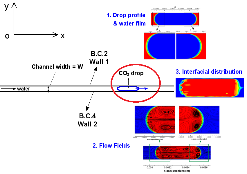
Simulation results and relevant discussions are provided in this part. We first introduce the first stage of the computation for one specific case as well as the following stage, namely, CO2 drop flowing stage. Also introduced in the first part is the formation of a complete water film near the wall spanning from the front meniscus to the end meniscus of the drop. Secondly, flow fields within the CO2 drop and near the interface during the second stage of all computations are shown and analyzed. Lastly, we show the interfacial distribution profile of CO2 during the second stage which is subject to collaborating interphase diffusion and local convections.
3.1. CO2 Drop Preparation and Thin Film Formation
None of the commonly used geometries in microfluidics are used to produce the CO2 drop in our simulation work. Instead, an initialized CO2 drop by adapting one specific region that is close to the inlet of the channel with CO2 properties (i.e., density, viscosity, diffusivity, velocity) is employed to provide the CO2 drop (see Figure 1, Table 1 and Table 2). Since interfacial tension between pure CO2 and water is considered in the simulation that treated as a source term in the momentum equation, as shown by Equations (6)–(10), a typical cylindrical drop profile is expected. Nevertheless, a certain period of computation time is required for the interfacial tension to show effects.
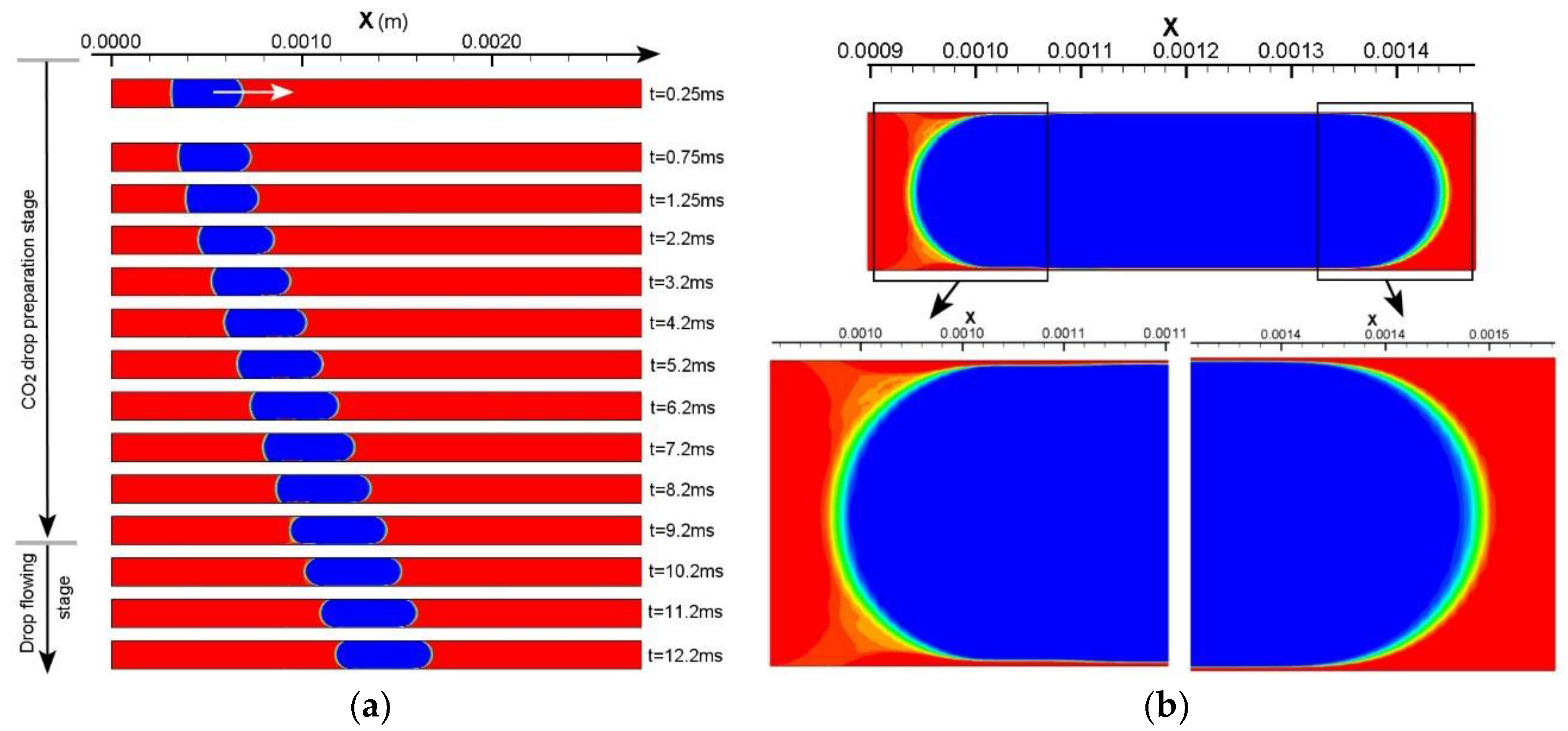
Taking Case 1 as an example, the first stage of computation for preparing a completely cylindrical profile of the drop is presented in Figure 2a. The initialized (liquid) CO2 drop is 0.3 mm from its left boundary to the channel inlet and assigned a velocity of 0.1 m/s which equals to that of water. The initial profile of this drop is a perfect quadrilateral. After 0.25 ms, the front boundary of the drop shows a bending effect, so does the back boundary with a slightly lower degree. As the computation proceeds, water films start to form at the front part of the drop near the channel wall which separate the drop from contact with the wall. The films continue to grow and extend to the back part of the drop. At t = 9.2 ms (i.e., Δt0 = 9.2 ms), a completely cylindrical profile of the CO2 drop is shaped (see Figure 2b). Both the front and back of the drop are of a meniscus shape. The drop is separated from contact with the channel wall by two thin water films, as shown by the zoom-in views in Figure 2b. The thin film thickness is measured 2~2.3 µm, i.e., 1.3~1.5% of the channel width (W). Based on the water properties in Table 2, the capillary number (Ca = µu/σ) of flowing water is 2.8 × 10⁻³ which results in a film thickness of ~2% W.
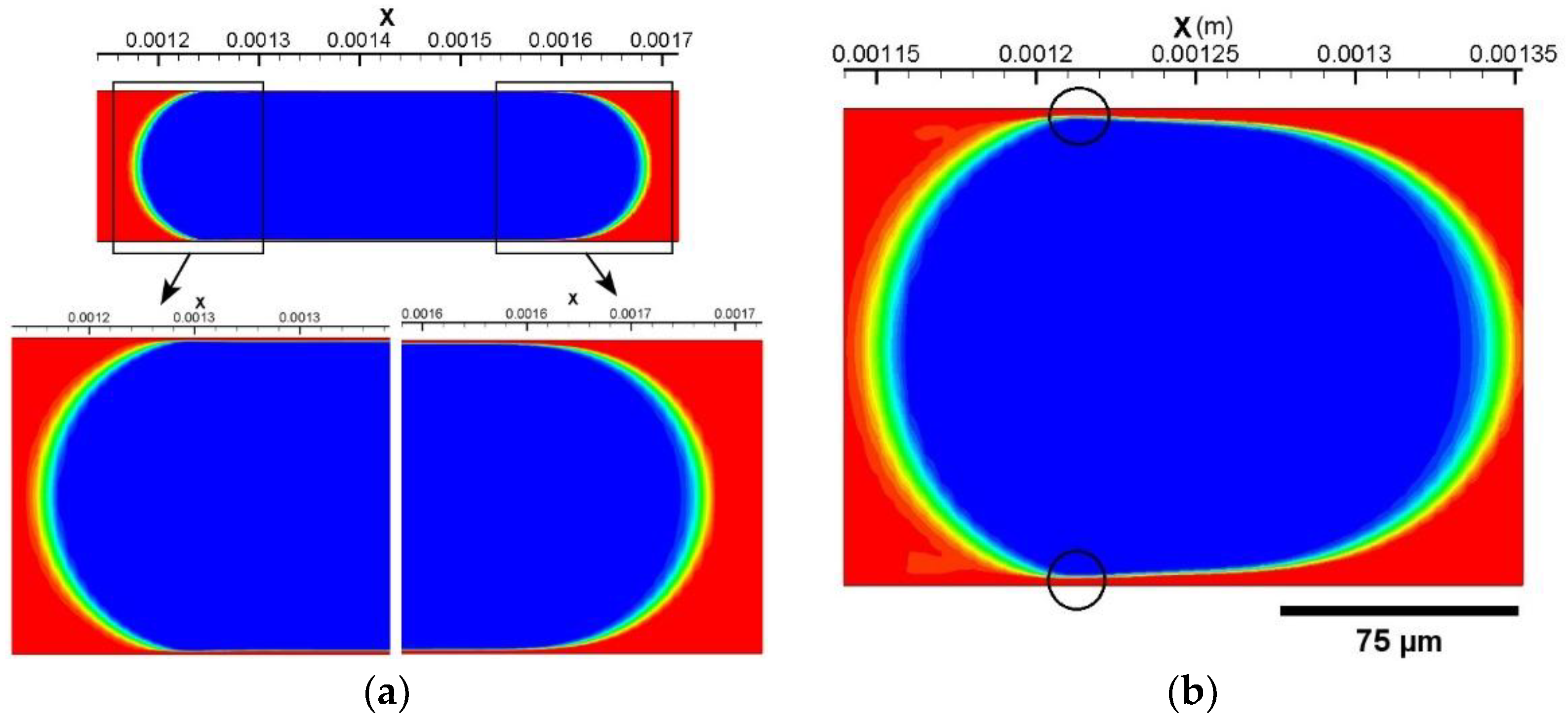
Three additional frames of the liquid CO2 drop at t = 10.2 ms, t = 11.2 ms, and t = 12.2 ms are provided in Figure 2a. The purpose is to showcase a stabilized thin film as well as stabilized front and back meniscus following the formation of these drop features at t = 9.2 ms, which legitimates dedicating t = 9.2 ms as an indication of the end of the CO2 drop preparation stage. Figure 3a shows the profile of the liquid CO2 drop at t = 12.2 ms, the drop length from the back to the front vertex of the meniscus is approximately equivalent to that at t = 9.2 ms (in Figure 2a). The thin film thickness (measured from the two bottom frames in Figure 3a) is 2.09 ± 0.06 µm on average which agrees with the 2~2.3 µm which has been measured at t = 9.2 ms.
Based on the above strategy to define the completion of the CO2 drop preparation, the other five simulation cases are analyzed as well. Three key parameters at the moment of the end of the first stage, i.e., the time duration (Δt0) of drop preparation stage, drop length (L0) at the end of this stage, and the film thickness (tfilm), are summarized (see Table 3). As introduced above, (x1 − x0) is the length of the initialized drop in a quadrilateral shape. However, during the drop preparation stage, there are certain expansions of initialized drops due to the effects of interfacial tension and pressure difference across the interface. Thus, the length of the prepared CO2 drop is generally greater than the initial one, as shown in Table 3. Furthermore, the deviation between (x1 − x0) and L0 is less significant for scCO2 drops than for liquid CO2 drops, which is attributed to the slightly higher interfacial tension of the scCO2 and water.
Besides, time durations (Δt0) of the CO2 drop preparation stage are also listed. The determination of Δt0 is analogous as in simulation Case 1. Regardless of the value of Δt0, they are small compared with the expected time duration of the second stage of the computation, namely, the drop flowing stage. The comparison can be carried out by Δt0/(Lt/ − Δt0) which is well below 7.5% for all cases.
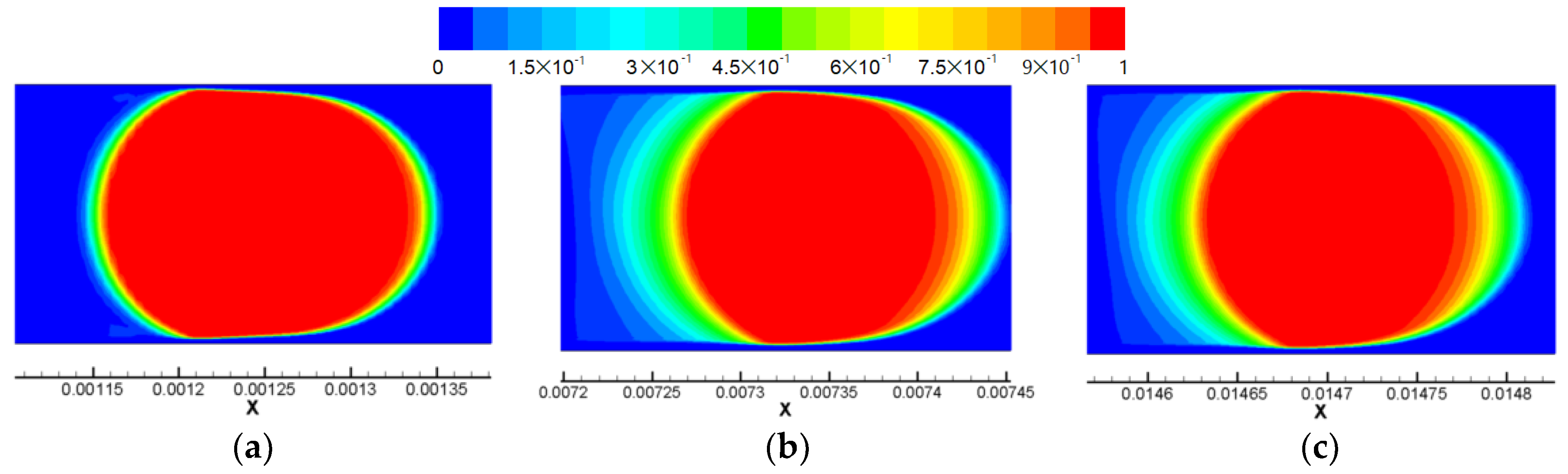
The thin film thickness in all simulation cases are measured and shown in Table 3. They generally range from 2 µm to 2.5 µm for most cases. Uniquely, Case 6 is characterized by a minimum film thickness of 3.36 µm at the narrowest position. This increased film thickness results from a short and bullet-shaped scCO2 drop in this case, which is rooted in an increased Ca (approaching 10−2) due to a higher fluid velocity. Figure 3b presents the drop profile of the prepared scCO2 drop in Case 6. It shows a difference in curvature between the front and the back meniscus of the drop and thus showcases the bullet-like drop profile. Two circles are added in the image to demonstrate the positions at which the film thickness is measured. Note that the two positions provide the minimum film thickness in this simulation case, even though it is larger than those of the drops in the other five cases. Although Case 6 is only one case of a high flow velocity being considered, the same drop profile and increased film thickness are anticipated for even higher flow velocities resulting in capillary numbers ~10−2.
3.2. Flow Fields within CO2 Drops and Near the Interface
Segmented flow or Taylor flow in microchannels has been placed with great expectations to enhance heat and mass transfer between phases such as gas–liquid and liquid–liquid. One important reason among others (e.g., high surface–volume ratio, short transport distance) is the convective hydrodynamics within the drop or bubble as well as those lying in both sides of the interface between phases. This feature is helpful in enhancing the transport of thermal energy and mass by collaborating with diffusion. Thus, flow fields within discrete segments and slugs particularly in the vicinity of the segment meniscus have become an interesting research topic in recent years.
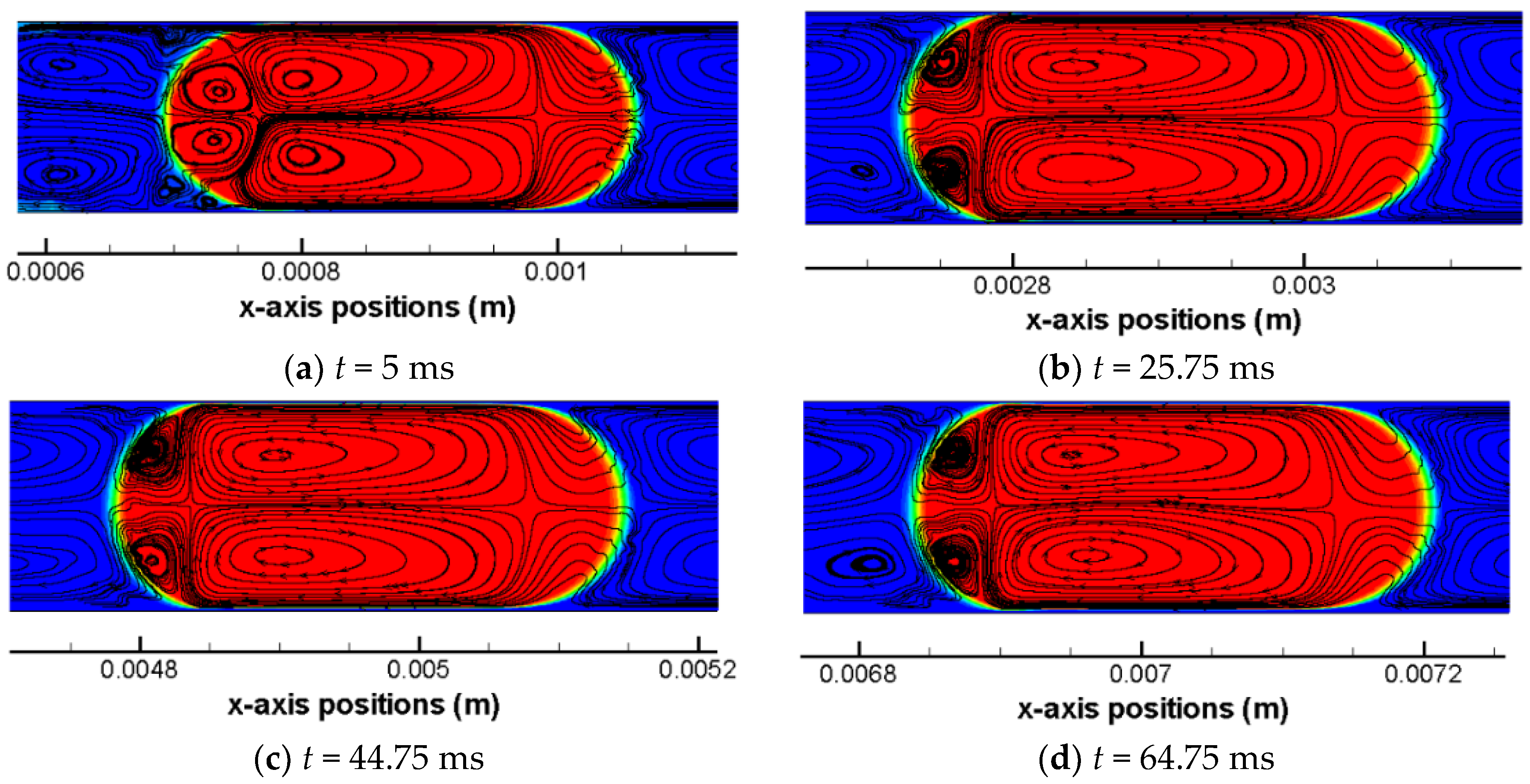
CO2 molecules are able to enter into the solvent phase (e.g., water) driven by diffusion and convection. As a consequence, the shrinkage of CO2 drop occurs, as reported previously [18,19]. However, it is technically challenging and demanding to experimentally probe the flow fields within droplets. An alternative is numerical simulation. Figure 4 shows the flow streamlines within the scCO2 drop and in the vicinity of the interface at the drop meniscus at eight time moments during the drop flowing stage. The streamlines are plotted in a frame of reference of the CO2 drop based on: (1) relative x-axis velocities that are calculated by subtracting the mean flow velocity (i.e., = 0.11 m/s) from computed x-axis velocities; and (2) y-axis velocities.
Focusing on the drop region (colored by red), there are generally four toroidal flow regions and one front region that can be identified. Two large vortex regions which are x-axisymmetric are located in the center of the CO2 drop. Along x-axis, these two regions share a same flow path that is identical to the bulk flow. However, the vortex direction are converse with each other—i.e., one is clockwise and the other is counter-clockwise—which has been caused by the local shear stress at the interface due to the presence of thin films. The shear stress of the drop at the interface are opposite to the drop flow and results in the tangential flow within the drop near the interface. Besides, there are two other vortices at the back meniscus of the CO2 drop that are x-axisymmetric as well and these two small vortices are in opposite directions too. At the back meniscus, the tangential flow velocity are dominated by the interfacial tension where shear stress becomes a weak role, as quantified by the local capillary number. At the front meniscus of the drop, no vortex region is observed and flows are in an opposite direction to the bulk drop flow. Due to the presence of the two larger vortex regions, the internal flow in the front region of the drop tends to be split and squeezed towards the thin film regions.
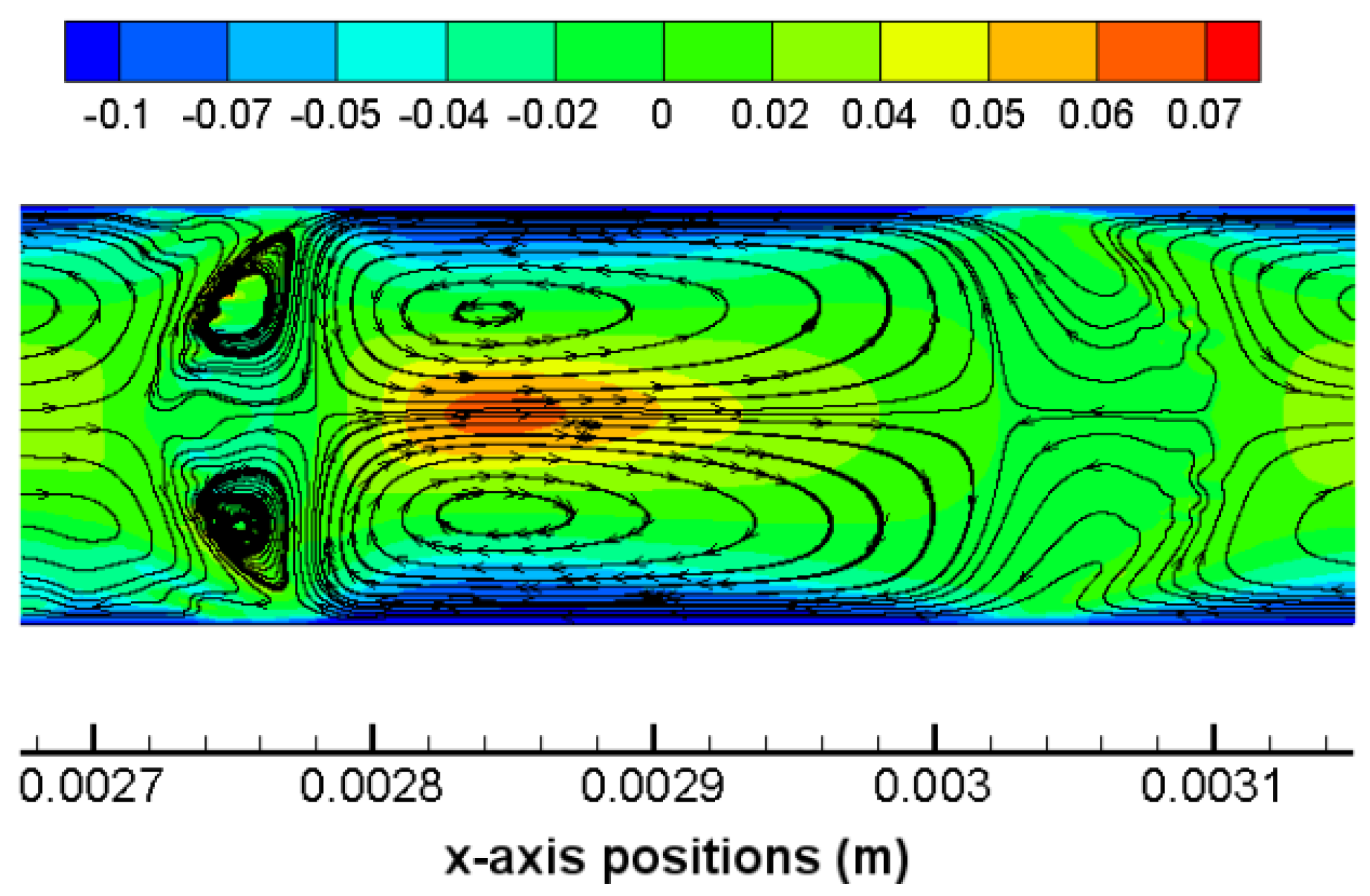
Out of the drop region, water slug regions in the vicinity of the back and the front meniscus of the drop are characterized by toroidal flow streamlines too, which can be found in all of the images in Figure 4. Near either the front or the back meniscus of the drop, there exist two vortex regions in the water slug which are in opposite directions and x-axisymmetric with each other. These vortices are formed due to combined effects of the shear stress (in negative-x direction) at the near-wall region and the net bulk flow (in positive-x direction) along the channel centerline under a presence of a drop meniscus. This elucidation is further clarified by the contour of relative x-axis velocities (partly based on which the flow streamlines are plotted) as shown in Figure 5. The blue region indicates that the thin water film as well as the boundary layer region (corner regions in Figure 5) near the wall are characterized by negative relative x-axis velocities. On the other hand, within the water region and on the axis, positive relative x-axis velocities are presented which indicate net bulk flows. These findings verify that shear stresses in near-wall regions are reverse to the bulk flow which further lead to the formation of flow vortices in water slugs.
According to Figure 4, the pattern of the flow field streamline within CO2 drop and near the interface are overall uniform among all studied time moments of simulation Case 4. It reflects that governing forces as well as their relative strengths during the drop flowing stage in the straight channel, quantified by a group of dimensionless numbers—such as Ca, Weber, and Re numbers—are overall constants in a steady hydrodynamic scenario in terms of flow velocities. The same situation in terms of a uniform pattern of flow streamlines within CO2 drops and near the interface, therefore, can be applicable to other five simulation cases (i.e., Case 1, 2, 3, 5, and 6) as well.
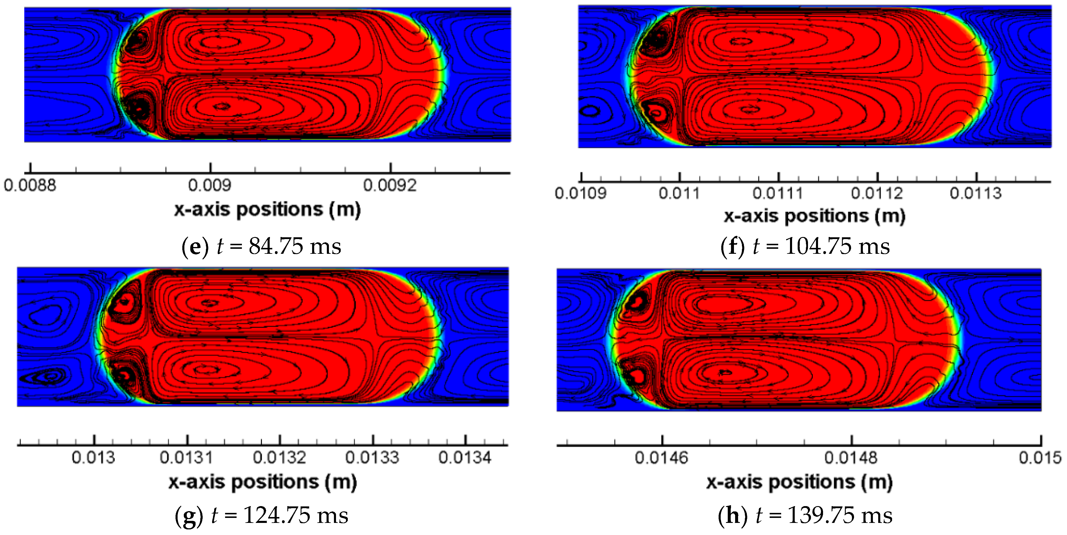
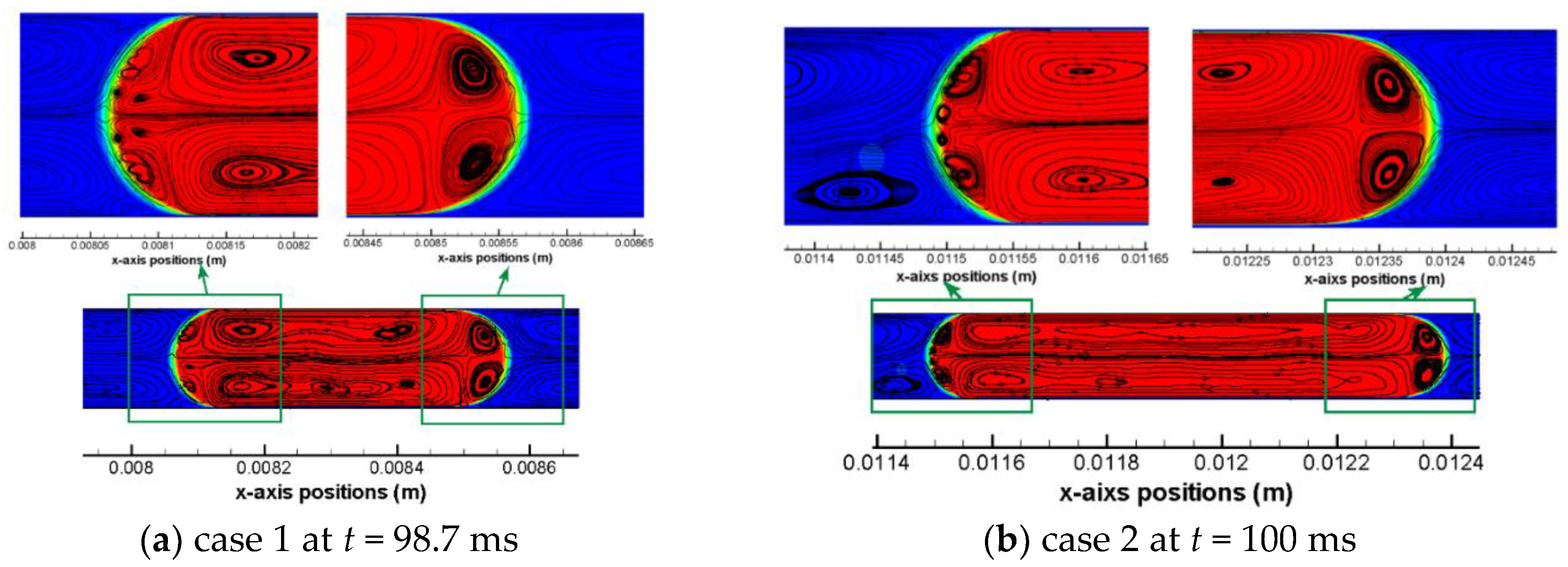
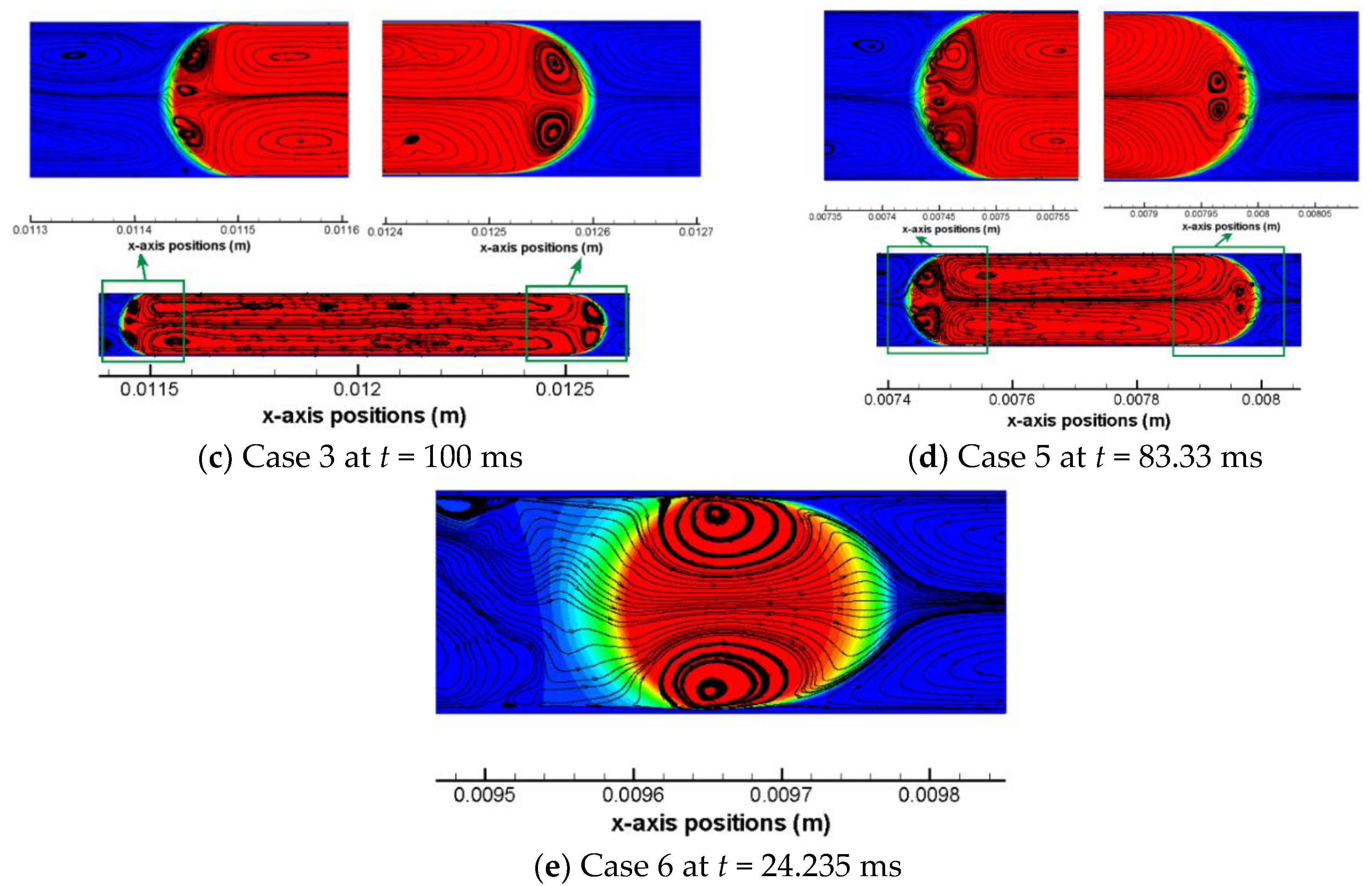
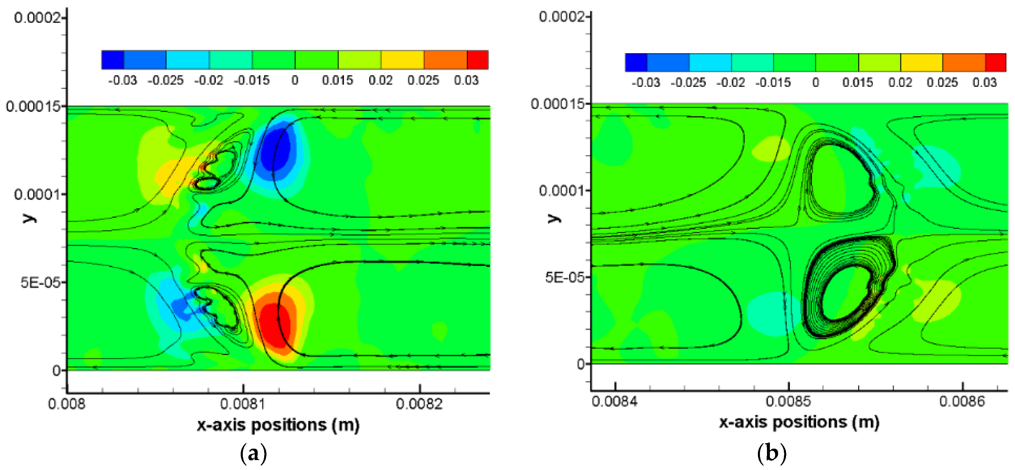
In view of a uniform pattern of flow streamlines for each simulation case, one time moment roughly during the middle of the a full computation process is chosen to present the characteristic flow streamline pattern for all cases, as shown in Figure 6. For liquid CO2 drops as shown by Figure 6a–c, a non-dimensional drop length (L0/W) has a range from 2.4 to 6.3. In addition, the capillary number of these three cases has an order of magnitude of 10−3. It is noticed that within both the front and the back meniscus of the drop there exists a pair of vortex regions, thus there are six vortex regions identified in total for these liquid CO2 drops. It is also clear that the front pair of vortex features a larger area than the back pair of vortex. Taking Case 1 as an example, y-axis velocities may be helpful to elucidate the vortex directions of the front vortex pair as well as the back vortex pair, as shown in Figure 7. It can be seen that across the interface there are always reverse y-axis velocities. In Figure 7a, colored small regions show a positive and a negative y-axis velocity in a neighboring domain across the meniscus. The reverse direction between these two small regions further results in a small vortex region in between of them. Note that this resulted small vortex region is still located within the CO2 drop. This inference (i.e., small vortex region in the drop meniscus resulting from the shear between inside of the drop and outside of the drop) is also applicable to the other pair of vortexes in the front meniscus domain, as that shown in Figure 7b. Based on observations from Figure 5, Figure 6 and Figure 7, it can be concluded that flow streamlines within the drop and near the interface are mainly caused by the shear including the shear stress in the thin film and that at the drop meniscus.
According to Figure 6, it can also be observed that there are multiple smaller vortex regions within the two larger vortexes in the middle of each Taylor liquid CO2 drop. These smaller vortexes may have been formed due to possible uneven shears from place to place along the interface of the long drop on the x-dimension while strong inertia always maintain as a constant on the axis of the drop. Similarly, six vortex regions are found in Case 5 (see Figure 6d), where the scCO2 drop has a non-dimensional length of 3.45 and a Ca number of 1.66 × 10⁻³. Despite a Ca number of 2.15 × 10⁻³ for Case 4, the Weber number (We = ρv2L/σ) is approximately 5.4 × 10⁻². By comparison, the inertia is 25 times larger than the viscous force, which can be actually quantified by the Re number (Re = We/Ca). Increased inertia find its influence on whether can vortex arise in the front meniscus of the drop. An extreme condition of scCO2 drop flowing at a very high velocity (~0.37 m/s) is provided by Case 6, as shown in Figure 3b and Figure 6e. The velocity increase has much more profound effects on inertia than on viscous forces, as formulated by Re number approaching 100 for the scCO2 drop in Case 6. The strong inertia does not lead to any formations of vortex in the drop meniscus domain. Nevertheless, shear stresses still dominate in the thin film region which are able to cause vortexes in the middle of the drop, as shown in Figure 6e.
3.3. Interfacial Profile of CO2 Drop
Mass diffusivity of liquid CO2 and scCO2 in water has been considered in the numerical simulation, see Table 2. These diffusivities are determined according to the Stokes–Einstein equation. Based on Equations (3) and (4), the diffusion of CO2 into water through the assumed “sharp interface” is considered in all simulation cases. Nevertheless, the diffusion should not be viewed as the only mechanism of CO2 transport.
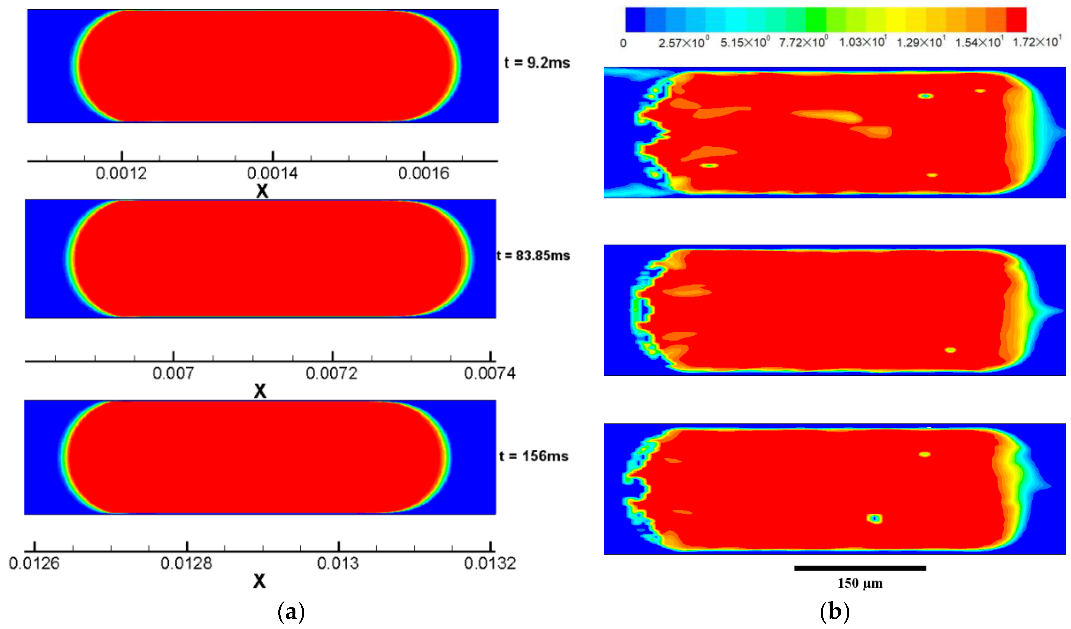
Using Case 1 as an example, Figure 8 presents comparisons of the drop profile of volume fraction (of CO2) and that of molar concentration of CO2 in water at three moments (i.e., at the beginning t = 9.2 ms, at the middle of this stage t = 83.85 ms, and at the end of the drop flowing stage t = 156 ms) of the drop flowing stage. Diffusion is generally weaker in mass transport compared with advection when these two mechanisms are collaborating in the transport process in the same direction. Here, the discussion of the CO2 transport are limited to the x-axis direction. Despite strong effects of the drop advection in the straight microchannel, the drop generally moves at the same pace as the continuously flowing water based on assigned velocities of these two phases, see Table 2. Therefore, the CO2 transport from its pure phase to water should first rely on diffusion (actually dissolution and diffusion, but dissolution is considered instant). At the front meniscus of the scCO2 drop, as shown in Figure 8b, the concentration gradient of CO2 which drives the diffusion is evident, as shown by the color change from red, yellow, green, and eventually to blue. However, evidenced by the vortex on the water slug side, as shown in Figure 6a, relative convections of the water flow from the channel wall towards the channel axis tend to flush the interface of the meniscus. Consequently, a distortion of the diffusional profile results from the neighboring convections. The distortion is justified by a triangular convex at the front meniscus of the drop (see Figure 8b). At the back meniscus of the drop, the profile of CO2 molar concentration is rather irregular. Different from at the front meniscus of the drop, convections here near the back meniscus are generally counteractive to the diffusion in terms of CO2 transport. Specifically, they are exactly opposite to diffusion on the axis, and at a bit deviated distance (a quarter of the channel width) from the axis, the opposing effects of convections are weakened due to a reduced x-axis velocity component and the diffusion here is less suppressed. Because of the varying relative strength of the diffusion compared with the local convections, the profile of CO2 molar concentration at the back meniscus generally presents a wavy pattern. In addition to the profile at the meniscus, the concentration as well as the concentration gradient of CO2 in the thin film region are almost zeros. This result is not very surprising since the convections in the thin film region are extremely rapid in transporting the diffused CO2 though the flow near the wall is typically slow than that in the middle of the channel.
Although not shown here, the CO2 concentration profile at the interface between the CO2 drop and water for all other CO2 drops in Cases 2, 3, 4, and 5 are the same based on the flow field streamline in Figure 6. A different interfacial profile at the front meniscus of the scCO2 drop in Case 4 may exist, for which flow streams originate from the water side and proceed into the drop through the meniscus, see Figure 4 and Figure 6. Since the flow streams are opposing to the diffusion in this region, the CO2 molar concentration profile could be significantly suppressed by the reverse convections.
The other distinct CO2 distribution profile emerges in simulation Case 6. According to Figure 6e. There are only two vortex regions in the middle of the drop and no vortex is found in the meniscus region. This is due to the relative small y-axis velocity compared with the x-axis velocity. As discussed in previous sections, the neglected y-axis velocity, despite some differences of it across the meniscus, is not likely to induce vortex inside the meniscus. In fact, relative x-axis velocities dominate the flow stream in the central region of the scCO2 drop. Additionally, there are very rare relative convections between water and CO2 due to the quite uniform x-axis velocity. Figure 9 shows the scCO2 drop in Case 6 at three different moments. Instead of CO2 molar concentration, the volume fraction of CO2 is utilized to identify the scCO2 drop. As soon as the scCO2 drop is prepared during the first stage of the computation, the diffusive ring surrounding the scCO2 drop is quite thin. However, as computation continues, the diffusive ring becomes wider over the x-dimension. Also, significant wide regions of volume fraction gradients at the front and the back meniscus of the drop can be observed, as shown in Figure 9b,c. The unidirectional gradient indicates that diffusion may be the only effective transport mechanism for CO2 into water as scCO2 drop moves at a very high velocity. This diffusion-only scenario can be comprehended based on above discussions about the involved flow streamlines. As now, relative x-axis velocities override the difference of y-axis velocities, resulting in no formations of vortex in the meniscus region of the drop. On the other hand, the dominant x-axis velocity is so uniform that any significant relative convections between water and CO2 do not exist. Thus, the effects of convection become subtle in a relative sense and diffusion becomes the only effective mechanism of CO2 transfer into water.
According to Figure 9, the length (Ldrop,x) of scCO2 drop at these three time moments are determined based on a nominal drop defined by a 0.5 cut-off volume fraction. The decreasing length demonstrates the shrinkage of this scCO2 drop over time. The computed drop length is first normalized by the channel width (W = 150 µm) and is then compared to the experimental result in the case QCO2/QH2O = 50/280, as presented in Figure 10. Generally, the simulated drop length overestimate the experimental drop length. However, the decreasing tendency over time is well predicted. Note that the first drop length in the simulation originates from the drop initialization in which an initialized drop length is referred to the experimental drop length and is applied in our simulation. If the computed scCO2 drop length is precisely predicted, it may enhance the predication further.
4. Discussions on Limitations of the Numerical Simulation
Despite successes in formations of CO2 drops and thin water film and in revealing the interfacial profile of the CO2 drop, our simulations here are still somewhat limited on several aspects, as follows: (1) 2D not 3D: it is a 3D scenario in a real flow situation of CO2 drop in the long straight microchannel, and it will be more informative to show the relevant results on the depth dimension even though longer computation time are required; (2) no droplet generation geometries (e.g., a T-junction) are considered, instead a CO2 drop preparation stage is introduced and applied, which might be a waste of the computation over this time period; (3) our simulation results are not fully validated by any experimental results yet. However, we note that any adequate experimental techniques—e.g., confocal microscopy and micro particle imaging velocimetry (µPIV)—are very performance demanding.
5. Conclusions
Here we present a numerical study on one single flowing liquid CO2 and scCO2 drop in a straight microchannel. Six simulation cases in total, including three (Cases 1 to 3) for liquid CO2 drop and three (Cases 4 to 6) for scCO2 drop, are considered. Each case is analogous to the corresponding experimental condition in terms of the flow property and the physical property of the CO2 and water, as shown in Table 1 and Table 2. Based on the numerical method introduced in Section 2, three main governing equations are introduced and applied, including: (1) a volume fraction equation (Equation (1)); (2) a continuity equation with respect to the two phases (Equation (3)); and (3) an overall momentum equation of one-single fluid (Equation (6)). Diffusivities of liquid CO2 and scCO2 in water are considered. The interfacial tension between CO2 and water is considered as a body force in the momentum equation. The numerical problem is formulated as 2D and transient. A pressure–velocity coupling algorithm is applied to solve the governing equations. Main simulation results are summarized in the following.
The computation of each simulation case is composed of two sequential stages, namely, the first stage—CO2 drop preparation stage and the second stage—CO2 drop flowing stage. A full liquid CO2 drop preparation stage for case 1 is shown, during which a cylindrical drop with two meniscuses at the front and the end of the drop is formed. Besides, thin water films on two sides of the drop near the channel wall are formed which separate the CO2 drop from contact with the wall. Generally, the drop preparation stage in all cases is <7.5% of the entire computation time. The thin film thickness ranges from 2 to 2.5 µm for all Taylor drops (in Cases 1 to 5) and is the largest (3.36 µm) in Case 6 which is characterized by the highest capillary number (~10−2).
Flow fields within the CO2 drop and near the interface are probed. For the CO2 drop in all the simulation case, there are generally two major toroidal vortex regions in the middle of each single drop, which is attributed to the significant shear stress in the thin film region as well as upon the interface. This inference is justified by the tangential flow stream of the vortex toroid at the interface which is always consistent with the shear stress in terms of direction. Moreover, small vortex regions are identified at the front and the back meniscus of the CO2 drops in typical Taylor drop flows (Cases 1, 2, 3, and 5). Their formations are due to the reverse velocity component on y-dimension between the inner drop and out of the drop. However, as the superficial velocity of the drop (as well as that of water) increases, small vortex regions start to vanish, first at the front meniscus of the drop as shown in Case 4 and later at both the front and the back meniscus of the drop. The vanish of small vortex in meniscus regions result from the weakening effects of y-dimensional velocities under increasingly dominant x-axis velocities in Case 4 and Case 6, as more revealed in Case 6 in which only major vortexes in the middle of the scCO2 drop are remained. In spite of this, increasing strengths of inertia relative to viscous forces in those regions are deemed the underlying causes.
Interfacial profiles of the CO2 drop are revealed. Diffusions tend to lead to one-dimensional concentration gradient starting from the initialized sharp interface. However, local convections near the interface are able to contribute to the CO2 distribution as well. Specifically, radially inward convections outside the front meniscus of the drop at water side induce a distortion of the diffusional profile and an approximately triangular convex of the concentration profile is formed. At the back meniscus of the drop, local convections generally show counteractive effects to the diffusion. Uneven relative strengths of convections in comparison with diffusion lead to irregular wavy profiles of the interfacial profile of the CO2 drop. The CO2 distribution profile in Case 1 may also be applicable to other Taylor drop flow cases—such as Cases 2, 3, and 5—in which local y-dimensional velocity components are comparable to the relative x-axis velocity in terms of magnitude in the vicinity of the drop meniscus. Case 4 and Case 6 characterized by higher x-axis velocities, relative convections between the CO2 side and water side turn out to be tiny. Thus, they contribute little to the CO2 transport from the drop to water. As of now, diffusion is the only effective mechanism controlling the CO2 transport, and an interfacial profile resulting from diffusion only is formed. Nevertheless, computed scCO2 drop length reductions in Case 6 are analogous to those reported previously [19].
Author Contributions
N.Q. and Y.F. conceived, designed, and performed the numerical simulations. N.Q. did the literature survey, data collection and analysis, and manuscript drafting/revising. Y.F. proposed the model and the meshing method. J.Z.W. and C.L.R. supervised and directed the project and reviewed the manuscript before submissions and resubmissions.
Conflicts of Interest
The authors declare no conflict of interest.
References
- Talimi, V.; Muzychka, Y.S.; Kocabiyik, S. A review on numerical studies of slug flow hydrodynamics and heat transfer in microtubes and microchannels. Int. J. Multiph. Flow 2012, 39, 88–104. [Google Scholar] [CrossRef]
- Erickson, D. Towards numerical prototyping of labs-on-chip: Modeling for integrated microfluidic devices. Microfluid. Nanofluid. 2005, 1, 301–318. [Google Scholar] [CrossRef]
- Gupta, R.; Fletcher, D.F.; Haynes, B.S. On the CFD modelling of Taylor flow in microchannels. Chem. Eng. Sci. 2009, 64, 2941–2950. [Google Scholar] [CrossRef]
- Wörner, M. Numerical modeling of multiphase flows in microfluidics and micro process engineering: A review of methods and applications. Microfluid. Nanofluid. 2012, 12, 841–886. [Google Scholar] [CrossRef]
- Hoang, D.A.; van Steijn, V.; Portela, L.M.; Kreutzer, M.T.; Kleijn, C.R. Benchmark numerical simulations of segmented two-phase flows in microchannels using the Volume of Fluid method. Comput. Fluids 2013, 86, 28–36. [Google Scholar] [CrossRef]
- Taha, T.; Cui, Z.F. Hydrodynamics of slug flow inside capillaries. Chem. Eng. Sci. 2004, 59, 1181–1190. [Google Scholar] [CrossRef]
- Fukagata, K.; Kasagi, N.; Ua-arayaporn, P.; Himeno, T. Numerical simulation of gas-liquid two-phase flow and convective heat transfer in a micro tube. Int. J. Heat Fluid Flow 2007, 28, 72–82. [Google Scholar] [CrossRef]
- He, Q.W.; Kasagi, N. Phase-Field simulation of small capillary-number two-phase flow in a microtube. Fluid Dyn. Res. 2008, 40, 497–509. [Google Scholar] [CrossRef]
- Yu, Z.; Heraminger, O.; Fan, L.S. Experiment and lattice Boltzmann simulation of two-phase gas-liquid flows in microchannels. Chem. Eng. Sci. 2007, 62, 7172–7183. [Google Scholar] [CrossRef]
- Falconi, C.J.; Lehrenfeld, C.; Marschall, H.; Meyer, C.; Abiev, R.; Bothe, D.; Reusken, A.; Schluter, M.; Worner, M. Numerical and experimental analysis of local flow phenomena in laminar Taylor flow in a square mini-channel. Phys. Fluids 2016, 28. [Google Scholar] [CrossRef]
- Mary, P.; Studer, V.; Tabeling, P. Microfluidic droplet-based liquid-liquid extraction. Anal. Chem. 2008, 80, 2680–2687. [Google Scholar] [CrossRef] [PubMed]
- Schuster, A.; Sefiane, K.; Ponton, J. Multiphase mass transport in mini/micro-channels microreactor. Chem. Eng. Res. Des. 2008, 86, 527–534. [Google Scholar] [CrossRef]
- Raimondi, N.D.; Prat, L.; Gourdon, C.; Cognet, P. Direct numerical simulations of mass transfer in square microchannels for liquid-liquid slug flow. Chem. Eng. Sci. 2008, 63, 5522–5530. [Google Scholar] [CrossRef] [Green Version]
- Shao, N.; Gavriilidis, A.; Angeli, P. Mass transfer during Taylor flow in microchannels with and without chemical reaction. Chem. Eng. J. 2010, 160, 873–881. [Google Scholar] [CrossRef]
- Onea, A.; Worner, M.; Cacuci, D.G. A qualitative computational study of mass transfer in upward bubble train flow through square and rectangular mini-channels. Chem. Eng. Sci. 2009, 64, 1416–1435. [Google Scholar] [CrossRef]
- Kececi, S.; Worner, M.; Onea, A.; Soyhan, H.S. Recirculation time and liquid slug mass transfer in co-current upward and downward Taylor flow. Catal. Today 2009, 147, 125–131. [Google Scholar] [CrossRef]
- Abolhasani, M.; Gunther, A.; Kumacheva, E. Microfluidic studies of carbon dioxide. Angew. Chem. Int. Ed. 2014, 53, 7992–8002. [Google Scholar] [CrossRef] [PubMed]
- Qin, N.; Wen, J.Z.; Ren, C.L. Hydrodynamic shrinkage of liquid CO2 Taylor drops in a straight microchannel. J. Phys. Condens. Matter 2018, 30, 094002. [Google Scholar] [CrossRef] [PubMed]
- Qin, N. Micro-Scale Studies on Hydrodynamics and Mass Transfer of Dense Carbon Dioxide Segments in Water. UWSpace. Available online: http://hdl.handle.net/10012/11940 (accessed on 12 March 2018).
- Brackbill, J.U.; Kothe, D.B.; Zemach, C. A continuum method for modeling surface-tension. J. Comput. Phys. 1992, 100, 335–354. [Google Scholar] [CrossRef]
Figure 1.
Schematic of the 2D computational domain for a single flowing liquid CO2 or scCO2 drop (outlined by either a rectangle at the left-hand side or a capsular shape in the middle and at the right-hand side) with water (regions outside of the drop) in a long straight microchannel (total length Lt = 15 mm and channel width W = 0.15 mm). The CO2 drop and water both flow from left to right. The origin of the coordinate is located at the center of the inlet, x-axis is in the channel length direction and y-axis is in the channel width direction. The drop here shows its presence at different moments.

Figure 2.
(a) The CO2 drop preparation stage of simulation case 1. Duration of this stage is Δt0 = 9.2 ms. (b) A completely cylindrical CO2 drop with two meniscuses is formed at t = 9.2 ms. Thin water film (as shown below) is 2~2.3 µm thick, compared to a 150 µm channel width. Red color indicates the volume fraction of water αH2O = 1, blue color indicates αH2O = 0 (i.e., αCO2 = 1).

Figure 3.
(a) A completely cylindrical CO2 drop is further stabilized at t = 12.2 ms. (b) The drop profile of the scCO2 drop in Case 6 at the end of the drop preparation stage. Two circles are added to indicate where the minimum film thickness is measured.
Figure 3.
(a) A completely cylindrical CO2 drop is further stabilized at t = 12.2 ms. (b) The drop profile of the scCO2 drop in Case 6 at the end of the drop preparation stage. Two circles are added to indicate where the minimum film thickness is measured.

Figure 4.
Flow field streamlines within the scCO2 drop and in the vicinity of the interface in simulation Case 4. The scCO2 drop is tracked over the drop flowing stage of the computation. Drop profile is presented at eight different time moments (a–h). Red color indicates αH2O = 1.
Figure 4.
Flow field streamlines within the scCO2 drop and in the vicinity of the interface in simulation Case 4. The scCO2 drop is tracked over the drop flowing stage of the computation. Drop profile is presented at eight different time moments (a–h). Red color indicates αH2O = 1.


Figure 5.
scCO2 drop at the moment t = 5 ms in simulation Case 4. Contours of relative x-axis velocities (absolute velocities subtracted by = 0.11 m/s) and flow streamlines are shown. Color levels of the band indicate the value of the relative x-axis velocity.
Figure 5.
scCO2 drop at the moment t = 5 ms in simulation Case 4. Contours of relative x-axis velocities (absolute velocities subtracted by = 0.11 m/s) and flow streamlines are shown. Color levels of the band indicate the value of the relative x-axis velocity.

Figure 6.
Representative pattern of flow streamlines within the CO2 drops and at the interface for all the other five cases (other than case 4), i.e., (a) Case 1; (b) Case 2; (c) Case 3; (d) Case 5; and (e) Case 6.
Figure 6.
Representative pattern of flow streamlines within the CO2 drops and at the interface for all the other five cases (other than case 4), i.e., (a) Case 1; (b) Case 2; (c) Case 3; (d) Case 5; and (e) Case 6.


Figure 7.
Contours of y-axis velocities and simple flow streamlines at (a) the back meniscus and (b) the front meniscus of the CO2 drop at time moment t = 98.7 ms in Case 1. Color bands on the top show the magnitude of y-axis velocity, m/s.
Figure 7.
Contours of y-axis velocities and simple flow streamlines at (a) the back meniscus and (b) the front meniscus of the CO2 drop at time moment t = 98.7 ms in Case 1. Color bands on the top show the magnitude of y-axis velocity, m/s.

Figure 8.
Liquid CO2 drop at three time moments (t = 9.2 ms, t = 83.85 ms, t = 156 ms) in simulation case 1. (a) Drop profile of volume fraction, red color indicates αCO2 = 1; (b) drop profile of molar concentrations of CO2 (cCO2) in water, color map on the top indicates the cCO2 value and red color indicates a nominal cCO2 of pure CO2 (i.e., cCO2 = ρ/M).

Figure 9.
scCO2 drop at three moments in simulation case 6. (a) t = 2.5 ms, Ldrop,x = (183 ± 4) µm; (b) t = 18.235 ms, Ldrop,x = (155 ± 5) µm; (c) t = 37.235 ms, Ldrop,x = (152.5 ± 3.5) µm. Color map shows the magnitude of the CO2 volume fraction, in which red color indicates αCO2 = 1.
Figure 9.
scCO2 drop at three moments in simulation case 6. (a) t = 2.5 ms, Ldrop,x = (183 ± 4) µm; (b) t = 18.235 ms, Ldrop,x = (155 ± 5) µm; (c) t = 37.235 ms, Ldrop,x = (152.5 ± 3.5) µm. Color map shows the magnitude of the CO2 volume fraction, in which red color indicates αCO2 = 1.

Figure 10.
Dimensionless scCO2 drop length (Ldrop,x/W) comparison between simulation results (open circles) at t = 2.5 ms, 18.235 ms, and 37.235 ms in Case 6 and experimental results (solid circles) at QCO2/QH2O = 50/280 [19] when scCO2 drop has a total flow time of 40ms in the straight channel.
Figure 10.
Dimensionless scCO2 drop length (Ldrop,x/W) comparison between simulation results (open circles) at t = 2.5 ms, 18.235 ms, and 37.235 ms in Case 6 and experimental results (solid circles) at QCO2/QH2O = 50/280 [19] when scCO2 drop has a total flow time of 40ms in the straight channel.


Table 1.
Simulation cases for a single flowing liquid CO2 and scCO2 drop.
| Parameters | Liquid CO2 Drop | scCO2 Drop | ||||
|---|---|---|---|---|---|---|
| Case 1 | Case 2 | Case 3 | Case 4 | Case 5 | Case 6 | |
| QCO2/QH2O (µL/min/µL/min) | 45/55 | 65/35 | 75/25 | 20/80 | 45/55 | 50/280 |
| x0 (mm) | 0.3 | 0.3 | 0.3 | 0.2 | 0.2 | 0.2 |
| (x1 − x0) (mm) | 0.36 | 0.72 | 0.942 | 0.33 | 0.517 | 0.16 |
| (m/s) | 0.1 | 0.11 | 0.11 | 0.11 | 0.085 | 0.3686 |
| (m/s) | 0.1 | 0.11 | 0.11 | 0.11 | 0.085 | 0.3686 |
Table 2.
Material properties of the applied water and CO2.
| Material Properties | Liquid CO2 Drop | scCO2 Drop | |||||
|---|---|---|---|---|---|---|---|
| Case 1 | Case 2 | Case 3 | Case 4 | Case 5 | Case 6 | ||
| QCO2/QH2O (µL/min/µL/min) | 45/55 | 65/35 | 75/25 | 20/80 | 45/55 | 50/280 | |
| Water | density (kg/m3) | 1004 | 1004 | 1004 | 995.61 | 995.59 | 995.63 |
| viscosity (µPa∙s) | 930 | 930 | 930 | 653.66 | 653.66 | 653.66 | |
| CO2 | density (kg/m3) | 755.23 | 755.23 | 755.23 | 311 | 309.07 | 315.4 |
| viscosity (µPa∙s) | 65.76 | 65.76 | 65.76 | 23.89 | 23.975 | 24.11 | |
| diffusivity (10−9 m2/s) | 1.79 | 1.79 | 1.79 | 58.193 | 58.423 | 57.666 | |
| Interfacial tension (mN/m) | 33.2 | 33.2 | 33.2 | 33.47 | 33.47 | 33.47 | |
| Contact angle (°) | 150 | 150 | 150 | 141 | 141 | 141 | |
Table 3.
Time duration of the drop preparation stage (Δt0), drop length (L0) at the end of preparation stage, and the film thickness (tfilm) of case 1 to 6. (x1 − x0), as an initialized drop length, is compared to the computed drop length L0.
Table 3.
Time duration of the drop preparation stage (Δt0), drop length (L0) at the end of preparation stage, and the film thickness (tfilm) of case 1 to 6. (x1 − x0), as an initialized drop length, is compared to the computed drop length L0.
| Parameters | Single Liquid CO2 Drop | Single scCO2 Drop | ||||
|---|---|---|---|---|---|---|
| Case 1 | Case 2 | Case 3 | Case 4 | Case 5 | Case 6 | |
| QCO2/QH2O (µL/min/µL/min) | 45/55 | 65/35 | 75/25 | 20/80 | 45/55 | 50/280 |
| (x1 − x0) (mm) | 0.36 | 0.72 | 0.942 | 0.33 | 0.517 | 0.16 |
| Δt0 (ms) | 9.2 | 10.5 | 14 | 4.5 | 9 | 2.5 |
| L0 (µm) | 540 | 915.5 | 1192.5 | 373 | 567 | 203 |
| tfilm (µm) | 2.03 ± 0.08 | 2.30 ± 0.09 | 2.48 ± 0.01 | 2.45 ± 0.005 | 2.30 ± 0.08 | 3.36 (narrowest) |
© 2018 by the authors. Licensee MDPI, Basel, Switzerland. This article is an open access article distributed under the terms and conditions of the Creative Commons Attribution (CC BY) license (http://creativecommons.org/licenses/by/4.0/).
Share and Cite
MDPI and ACS Style
Qin, N.; Feng, Y.; Wen, J.Z.; Ren, C.L. Numerical Study on Single Flowing Liquid and Supercritical CO2 Drop in Microchannel: Thin Film, Flow Fields, and Interfacial Profile. Inventions 2018, 3, 35. https://doi.org/10.3390/inventions3020035
AMA Style
Qin N, Feng Y, Wen JZ, Ren CL. Numerical Study on Single Flowing Liquid and Supercritical CO2 Drop in Microchannel: Thin Film, Flow Fields, and Interfacial Profile. Inventions. 2018; 3(2):35. https://doi.org/10.3390/inventions3020035
Chicago/Turabian StyleQin, Ning, Yu Feng, John Z. Wen, and Carolyn L. Ren. 2018. "Numerical Study on Single Flowing Liquid and Supercritical CO2 Drop in Microchannel: Thin Film, Flow Fields, and Interfacial Profile" Inventions 3, no. 2: 35. https://doi.org/10.3390/inventions3020035