Designing a Thermal Radiation Oven for Smart Phone Panels


1
Department of Mechanical Engineering, National Cheng Kung University, Tainan 701, Taiwan
2
Department of Power Mechanical Engineering, National Tsing Hua University, Hsinchu 300, Taiwan
3
C SUN Manufacturing Limited Company, New Taipei 241, Taiwan
*
Author to whom correspondence should be addressed.
Inventions 2018, 3(2), 36; https://doi.org/10.3390/inventions3020036
Submission received: 9 April 2018
/
Revised: 28 May 2018
/
Accepted: 30 May 2018
/
Published: 6 June 2018
(This article belongs to the Special Issue Heat Transfer and Its Innovative Applications)
Abstract
:Thermal radiation is the only heat transfer mechanism with vacuum compatibility, and it carries energy at light speed. These advantages are taken in this work to design an oven for smart phone panels. The temperature of panels is acquired from a numerical method based on finite-difference method. The space configuration of the heating lamps as well as the relative distance between lamps and the panel are control factors for optimization. Full-factorial experiments are employed to identify the main effects from each factor. A fitness function Q considering both temperature uniformity of the panel and the heating capability of the ovens is proposed. The best oven among 27 candidates is able to raise panel temperature significantly with high uniformity.
1. Introduction
Radiative heat transfer is one of three mechanisms that transfer thermal energy, and it has played a critical role in multiple applications for its uniqueness. Thermal radiation is composed of photons or electromagnetic waves emitted from a subject at a temperature greater than zero Kelvin [1]. When radiation is emitted from a relatively hot subject and absorbed by a colder one, heat is transferred successfully. Unlike the other two heat transfer mechanisms (heat conduction and convection), radiative heat transfer requires no intervening media. That is, thermal radiation is the only way to transfer heat in a vacuum. Moreover, heat travels at light speed, and its flux is positively correlated with the fourth power of absolute temperature. These characteristics have facilitated applications using thermal radiation in energy harvesting, temperature sensing, heating objects, and others [2,3,4,5,6,7,8,9,10,11].
Ovens simultaneously utilizing thermal radiation and convection are popular for material processing and food cooking. Thermal radiation is able to provide a large amount of heat at light speed, while the convection helps temperature uniformity via fluid motion [12,13,14]. The first oven using thermal radiation (infrared mainly) was patented in 1958 [14]. Many following studies and innovations further enhanced the performance and reduced their fabrication cost [15,16,17,18]. A recent example was the oven developed by Pakkala [18]. However, an oven using dual heat transfer mechanisms may not fit all heating process needs. The glass panels of smart phones are an example because their tolerance to particles is close to zero. A vacuum environment is necessary, and purely using thermal radiation becomes the only choice.
The objective of this work is thus to design an oven for smart phone panels, and the oven only employs thermal radiation for heating. The advantages of thermal radiation, namely vacuum compatibility and prompt heat transfer, will be fully employed. On the other hand, intrinsic drawbacks resulting from thermal radiation will be diminished. One drawback is the dependence of emission intensity on orientation and direction [1]. The other is uneven emissive power received on the panel surface. These drawbacks not only downgrade the temperature uniformity of the panel, but reduce its ultimate temperature. Attempts to fix the abovementioned drawbacks are briefed in the following. First, an oven containing heating lamps was numerically constructed in a model based on finite-difference method. Second, three control factors for optimization were selected from oven configurations. Three levels were then assigned to each factor such that the total number of oven configurations for testing was 27. Third, the temperature distribution of a panel was investigated in each test. A quantitative analysis was conducted through a full factorial experiment. Fourth, a fitness function Q was defined and utilized for quantitative evaluation of the oven performance. Performance and detailed configurations of the best oven among the 27 candidates is presented at the end of the manuscript.
2. Design Strategy
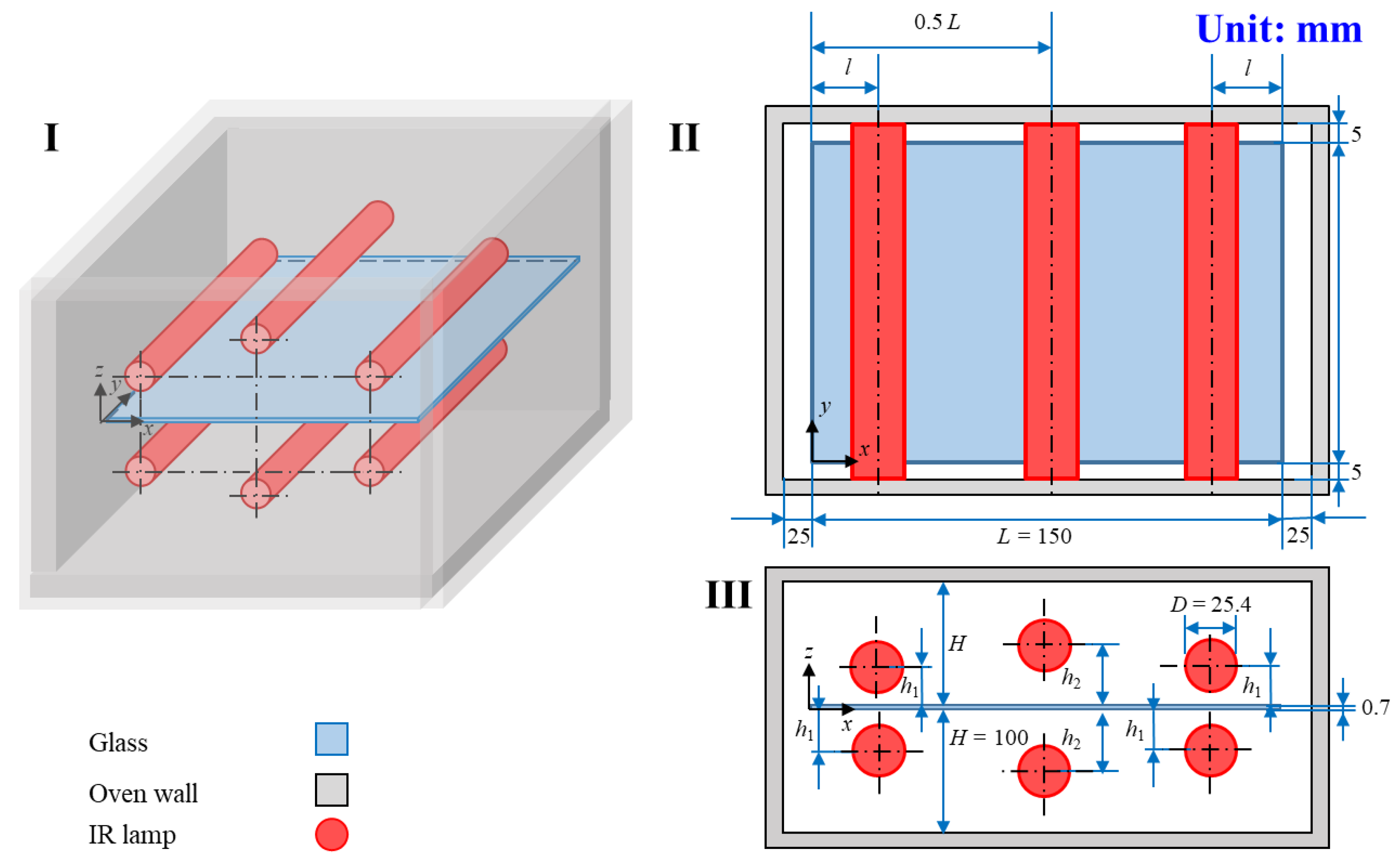
Figure 1 shows a sketch of the proposed thermal radiation oven, which is cuboid in appearance. It contains six lamps for heating a glass panel, as shown in subgraph I. The panel is placed horizontally in the middle of oven. Three lamps are located above and below the panel. Three lamps at one side and their counterparts at the other side are located symmetrically with respect to the panel. The middle lamp is directly above the center line of the panel. The other two are side lamps, and their alignment is symmetric with respect to the center plane defined by the centerlines of the middle lamp and the panel. Actually, the centerline of the oven is also on the center plane. Subgraph II shows the top view of the oven. The lateral dimensions of the panel are length L = 150 mm and width W = 70 mm. The gap between the edge of the panel and the oven wall is 25 mm for four sides. l symbolizes the horizontal distance between the center line of the side lamp and the edge of the panel. Subgraph III provides the front view of the oven. The vertical distance from the oven top or bottom to the panel is H = 100 mm. Since the panel is for a smart phone, the thickness is as little as 0.7 mm. The diameter of each lamp is D = 25.4 mm. h1 is the vertical distance between the center of a side lamp and the panel surface, while h2 is the vertical distance between the center of the middle lamp and the panel surface.
Table 1 lists three dimensionless control factors (l/L, h1/H, and h2/H) considered in modeling. Each control factor has three levels, and these levels form an arithmetic series. For l/L, the first level (Level 1) is zero. The center line of a side lamp is aligned along with a panel edge. As the level increases, side lamps get close to the middle one. The other two control factors are the vertical distance between lamps and the panel surface. h1/H and h2/H are the gaps associated with the side lamps and the middle one, respectively. The gap is enlarged as the level increases. Once the levels of all control factors were specified, the configuration of the oven was determined for testing. A test was then conducted numerically by heating a panel inside. Results were the temperature distribution at the top surface of the panel. Key quantitative data about the distribution was also recorded for analysis. One was ΔTmax, the maximum temperature difference within the surface, to reflect temperature uniformity. Another was Tavg, the average temperature over the surface. This value should be higher than panel’s initial temperature Tini after the panel is heated. Here, Tini = 25 °C was set to be the same as the temperature in the surroundings Tsurr and the commonly employed “room temperature”. The temperature difference (Tavg − Tini) can be viewed as the heating capability of an oven. For an ideal oven, temperature uniformity of the heated panel should be high, and heating capability of the oven should be as large as possible.
A dimensionless fitness function Q is defined below to quantitatively evaluate the performance of the oven in all tests:
where Q was first determined by ΔTmax. If it was larger than 20 °C, the temperature of the panel varied too much for the oven to be considered in further performance evaluation. As a result, Q was set to null. On the other hand, Q was calculated for the remaining tests with ΔTmax ≤ 20 °C. The calculation not only needs the denominator ΔTmax, but the numerator Tavg − Tini. Q is expected to be a large positive number for an ideal oven, which brings about uniform and high temperature within panels.
3. Numerical Model
3.1. Thermophysical Properties
Lamps at 500 °C were used as heating sources in our numerical model. The emissivity of their surfaces was assumed to be unity like a blackbody (i.e., εL = 1). The emission was partly absorbed by the glass (SiO2) panel. Its thermal conductivity k and diffusivity a at room temperature were k = 1.51 W/m·K and a = 8.34 × 10⁻⁷ m2/s, respectively [19]. Their variations with temperature were not considered in modeling because the amount was trivial. Clearly, the panel was not a good thermal conductor. Its temperature uniformity became critical for an oven using only thermal radiation.
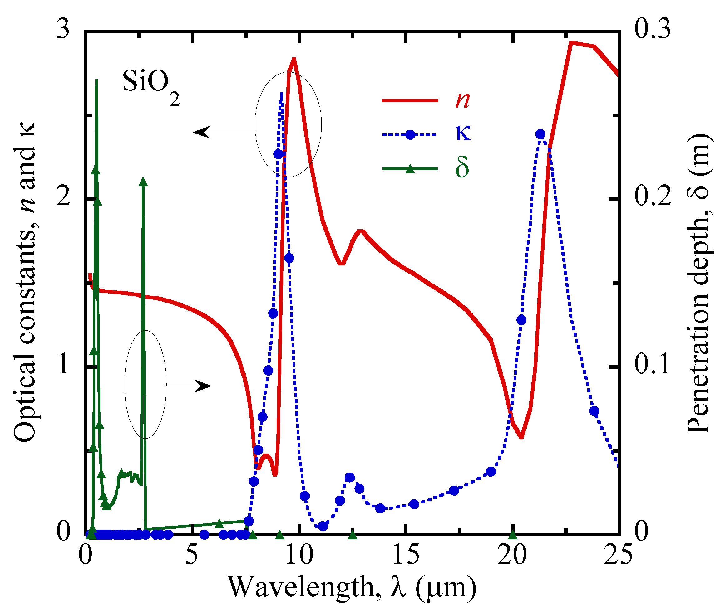
Figure 2 shows the optical constants (refractive index n and extinction coefficient κ) spectra of SiO2 [20]. The spectral range was from 0.2 μm to 20 μm, covering most of the emission spectra. These constants are employed later for calculating the spectral absorptivity αλ. When the wavelength was between 0.2 and 8 μm, the extinction coefficient κ was almost zero. The penetration depth δ = λ/4πκ was much greater than the thickness of the panel (0.7 mm), such that the panel was semi-transparent to emission. Conversely, as the wavelength λ was longer than 8 μm, the penetration depth δ was almost null. The panel became opaque to incident radiation, and the energy was either absorbed or reflected.
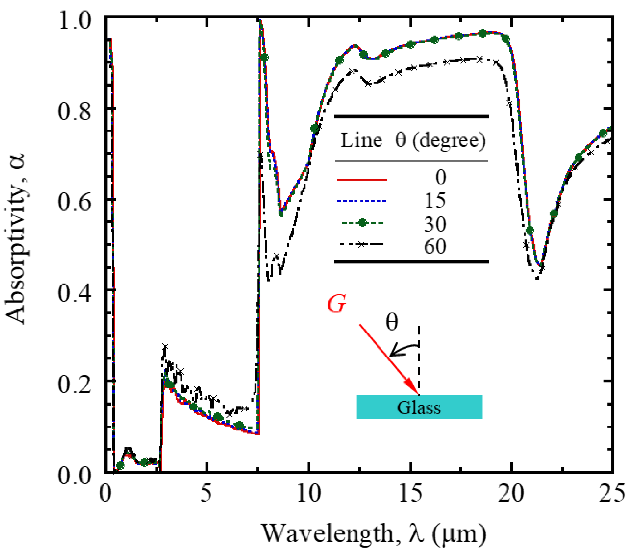
Figure 3 shows the absorptivity spectrum of a panel. Each plot corresponds to an incident angle θ = 0°, 15°, 30°, or 60°. Since the difference among plots is insignificant, the angular dependence of radiative properties was omitted in our model. On the other hand, wavelength-dependence was obvious such that a total radiative property was averaged over the spectral range. A spectral radiative property could be numerically obtained by solving Maxwell’s equations with the aforementioned optical constants [21]. The spectral absorptivity αλ was equal to the spectral emissivity ελ according to Kirchhoff’s law [19]. The spectrum could therefore be employed to obtain the glass emissivity. Note that the total absorptivity αtotal is not the same as total emissivity εtotal because temperature was different for the panel and lamps. The wavelength λ = 8 μm serves as a demarcation point in the figure. When λ < 8 μm, the glass absorptivity was low, but radiation power of the lamp was high, indicating that the absorption effect of the glass was poor in this range. When λ > 8 μm, the glass emissivity was high, indicating that the glass had high energy loss in this range. In particular, when 8 μm ≦ λ ≦ 10 μm or 20 μm ≦ λ ≦ 25 μm, the absorptivity attenuated significantly. The reason is the curves n and κ intersected in these two ranges. The radiative properties of the panel switched between those of a dielectric and a metal.
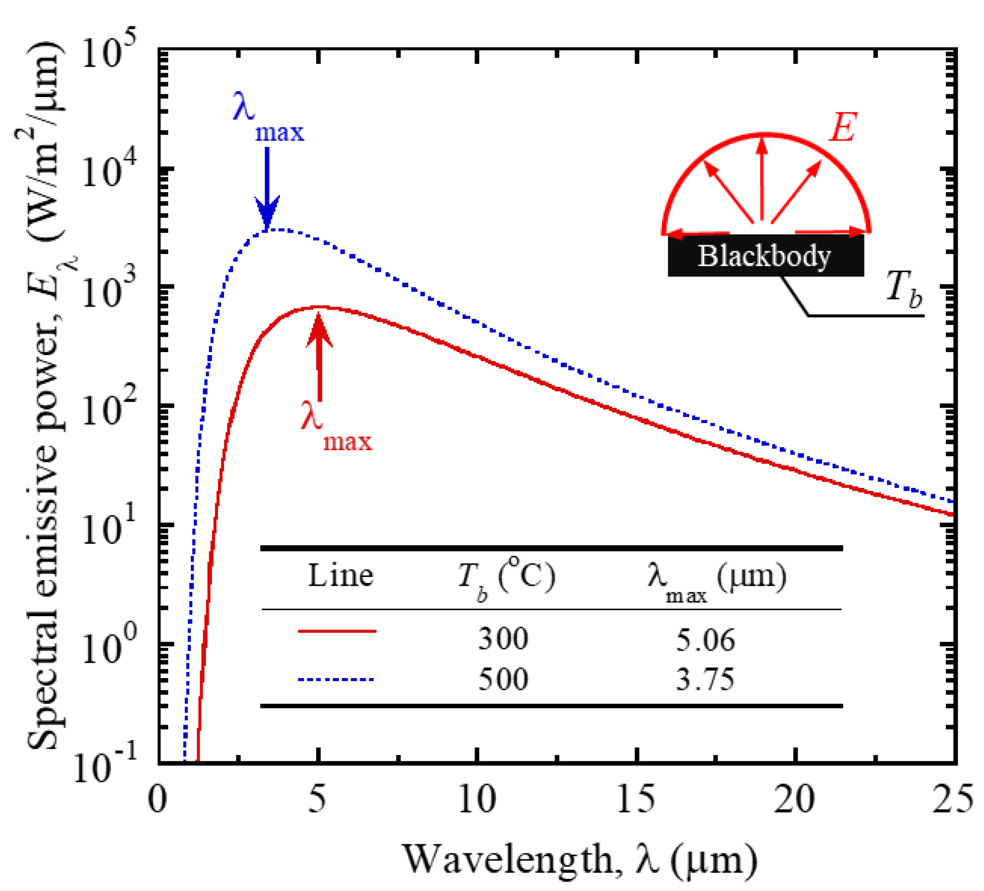
Figure 4 shows the spectral emissive power from a blackbody following Planck’s distribution [19]. The power at temperatures Tb = 500 °C and 300 °C were treated as the ideal radiation intensity of lamp and glass, respectively. The peak values of the two radiation intensities were at λ = 3.75 μm and λ = 5.06 μm, respectively, indicating that the main distribution range of radiation energy was around the peak point. In addition, the combined effect of the demarcation point of absorptivity and the spectral distribution of the black body radiation intensity was considered, and the blackbody radiative energy ratio (Equation (2)) was used as the basis for selecting the average band for total absorptivity and total emissivity of the glass.
where σ = 5.67 × 10⁻⁸ W/m2·K4 is the Stefan–Boltzmann constant, and C1 = 3.742 × 10⁸ W·μm4/m2 and C2 = 1.439 × 104 μm·K are the first and second radiation constants, respectively. According to calculation, when 0.2 μm ≦ λ ≦ 8 μm, the radiative energy ratio is . When 5 μm ≦ λ ≦ 25 μm, the radiative energy ratio is , indicating that the two bands are representative.
In summary, the total absorptivity αtotal = 0.17 in the band of 0.2 μm ≦ λ ≦ 8 μm was selected as representative of the glass absorptivity, and the total emissivity εtotal = 0.79 in the band of 5 μm ≦ λ ≦ 25 μm was selected as representative of the glass emissivity.
3.2. Finite-Difference Method
In the simulation analysis of temperature distribution, we used the finite difference method to directly analyze the steady state of panels. By assuming that the oven is internal heat-free and that the glass is homogeneous, isotropic, and stable, the energy equation can be reduced to Equation (3):
Then, Equation (3) can be converted into to Equation (4) according to the central difference method [22]. Equation (4) is then solved using the tridiagonal matrix algorithm for temperature T at node (i, j, k) and others. Solving this equation takes multiple iterations, and the iteration number is specified with superscript m. Iteration continues until temperature is converged at every node.
Four sides of the glass were assumed adiabatic as boundary conditions. Because the upper and lower surfaces were irradiated directly by lamps, they absorbed part of irradiation with total absorptivity αtotal. At the same time, the surfaces emitted thermal radiation to the environment with the total emissivity εtotal. Boundary conditions for these surfaces therefore included these parts and conduction as listed in Equation (5):
4. Results and Discussion
4.1. Program Convergence
Figure 5a displays the flow chart for the calculation program. Firstly, the infrared lamp, glass thermophysical properties, environmental thermophysical properties. Level of each control factor was assigned in the MATLAB program for obtaining temperature distribution of the panel by cyclic calculation. Secondly, by repeated iterations, results were output when they satisfied the following two criteria. Equation (6) is criterion one to assure the convergence of temperature at node (i, j, k). The maximum relative error of temperature Ti,j,k obtained from two successive iterations is less than 0.1%. Criterion two is to prevent the program from infinite iterations. The maximum number of iterations was set to 400,000. If the loop number does not provide temperature convergence, an error message will pop out.
Figure 5b chooses one of 27 combinations to make a grid convergence test. The control factors of this oven were l/L = 0, h1/H = 0.5, and h2/H = 0.5, and the grid sizes for the test were Δy = 1.75, 3.5, 7, and 14 mm, respectively. The upper and lower subgraphs show the convergence of the average temperature Tavg and the maximum temperature difference ΔTmax with the iteration number m, respectively. Results showed that the results of the previous four mesh sizes were all convergent when the number of iteration times m was about 300,000. In addition, the average temperature Tavg was consistent with the maximum temperature difference ΔTmax when the size of the grid was Δy ≤ 7 mm. To ensure convergence and consider the spatial temperature distribution resolution, the grid was set as Δy = 1.75 mm.
4.2. Temperature Distribution
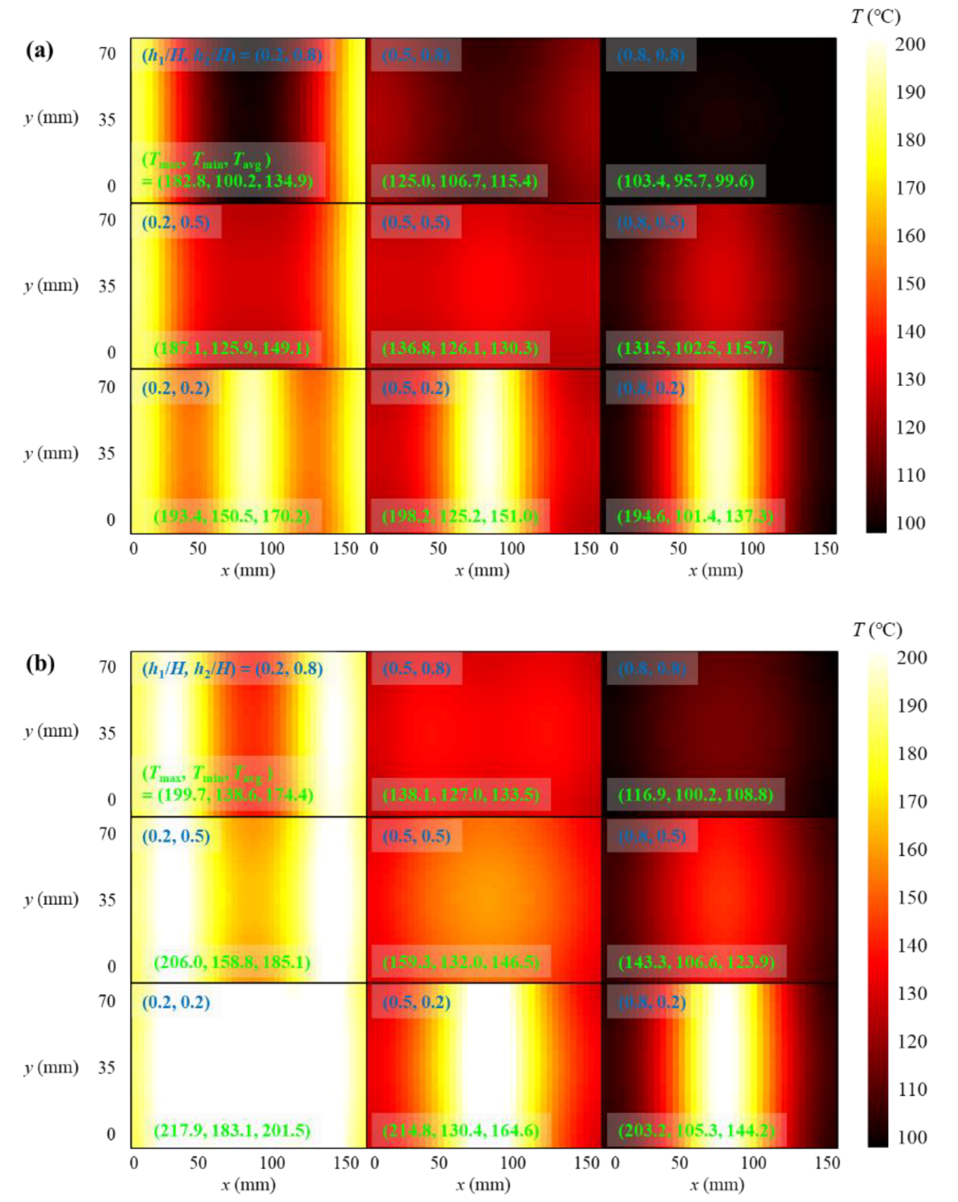
Figure 6 shows the temperature distribution of the panel surface based on Table 2. Subgraphs (a), (b), and (c) represent the temperature distribution when the control factor l/L was 0, 1/6, and 1/3, respectively. Each subgraph contains nine (3 × 3) temperature figures. The darkest and lightest colors correspond to 100 °C and 200 °C, respectively. Each row has the same control factor h1/H, and the three rows correspond to h1/H = 0.2, 0.5, and 0.8, respectively. Each column has the same number of h2/H, and the three columns from left to right correspond to h2/H = 0.2, 0.5, and 0.8, respectively. Each temperature distribution corresponding to the control factor is also marked blue in the upper-left corner, and the highest temperature Tmax, the lowest temperature Tmin, and the average temperature Tavg are marked in green in the lower-left corner.
In Figure 6a, when h1/H = h2/H = 0.2 (the temperature distribution in the lower-left corner of the figure), the glass had the highest average temperature (Tavg = 170 °C), because all the lamps were close enough to the glass surface that the panel was effectively heated. In contrast, the temperature distribution in the upper-right corner (h1/H = h2/H = 0.8) showed the lowest average temperature (Tavg = 99.6 °C) when all the lamps were far away from the glass. However, once the lamp was near the panel, the heat was concentrated below the lamps and the heat diffusion capacity of the glass is very low, forming a partial high temperature, such as the high temperature occurring under the central lamp in the third column (h2/H = 0.2), and the first line (h1/H = 0) showing the high temperature below the edge lamp. So, the compromise scheme is to improve the height of the lamp to h1/H = h2/H = 0.5, and the temperature distribution is shown in the second rows and second columns. In this figure, the temperature not only increased, but the distribution was also relatively uniform, indicating that the heat radiation energy emitted by all lamps was more evenly irradiated on the panel surface.
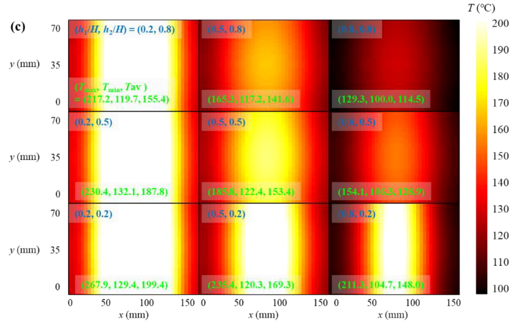
Figure 6b is the counterpart of Figure 6a. The difference is only that side lamps shrank to the center so that l/L = 1/6. In addition to finding the same result as Figure 6a, we could clearly see the effect of the two side lamps. The first effect was that the heating range of side lamp was also retracted, and the high-temperature region was concentrated in the center of the glass. For example, the central temperature distribution figure (h1/H = h2/H = 0.5) has a large pattern of high temperature in the center. The second effect was that the average temperature was also increased, so when h1/H = h2/H = 0.2, the maximum average temperature could even reach 201.5 °C. The third effect was that the temperature at the edge of the glass was also increased. The main reason is that the side lamps shrank, and more heat could be absorbed by the edge of the glass.
Figure 6c shows that the effect of the side lamps was more obvious, the highest temperature and the average temperature of the glass increased, which could reduce the temperature drop caused by increasing the distance between the lamps and the glass. For example, the average temperature of the first row third line (h1/H = h2/H = 0.8) increased to 114.5 °C, but the three lamps were too close to the glass, which made the heat concentrated in the middle of the glass line. This concentration caused the highest and lowest temperatures to be at the center and edge, respectively, so the temperature difference became larger. For example, in the first row of the third line (h1/H = h2/H = 0.2), the temperature difference could reach 138.5 °C, which is unacceptable for an oven.
4.3. Main Effects and Fitness Function
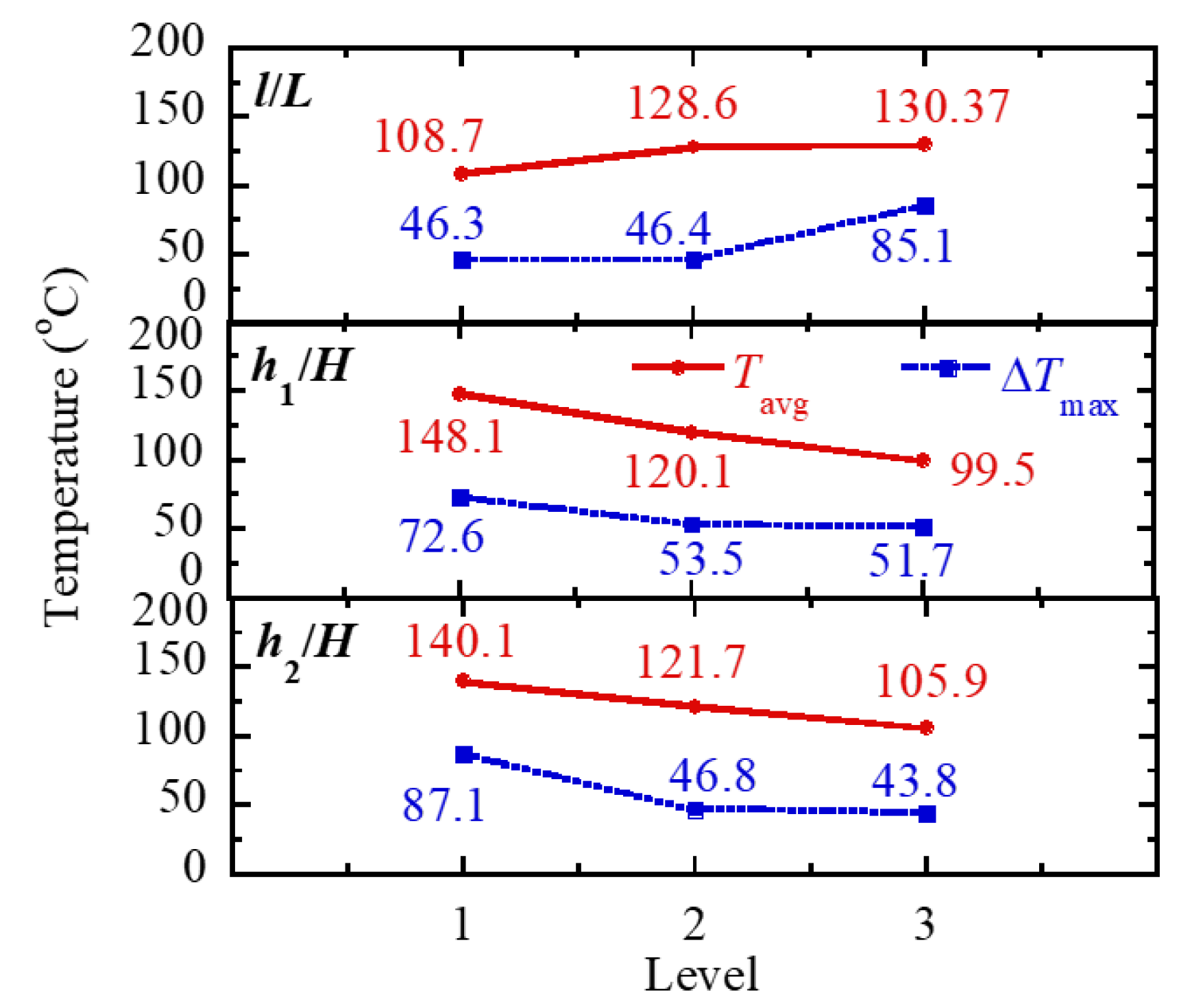
Figure 7 shows the main effects of each control factor to make a comprehensive comparison. The red line and the blue line represent the trend of the variation of control factors with the level of Tavg and ΔTmax, respectively. The numbers in the figure show the control factor’s effect, illustrating its calculation method: the Tavg value of l/L at Level 1 was 108.7, meaning the average value of Tavg in the l/L in line number 1 in Table 2. The results show that Tavg increased by 20 °C when the level of l/L rose from Level 1 to Level 2, but the ΔTmax only increased by 0.1 °C. When the level of l/L increased to Level 3, the variation of Tavg was not significant (<2 °C), but the ΔTmax obviously increased (>38 °C). This indicates that a moderate reduction in the distance between lamps could obviously increase Tavg without ΔTmax of the panel, but further decrease of the distance between lamps would not only yield a minor increase the average temperature, but lead to a sharp rise in the temperature difference. The best level of l/L was therefore l/L = 1/6 (Level 2). In terms of h1/H and h2/H performance, it was found that Tavg decreased monotonically when their levels increased. ΔTmax decreased obviously when the Level 1 was raised to Level 2, but ΔTmax changed little when it continued to increase to Level 3. This indicates that increasing the distance between the lamps and the glass is helpful to reduce the temperature difference, but will also decrease the average temperature. The best level of h1/H and h2/H was therefore h1/H = h2/H = 0.5 (Level 2).
However, when l/L was 1/6 and h1/H = h2/H = 0.5, the figure in the center of Figure 6b shows that ΔTmax was larger than 20 °C, so the combination l/L = 0 and h1/H = h2/H = 0.5 should be taken into account. Its temperature distribution figure shows more uniformity and the Tavg was not very low. So, the value of fitness function Q for each combination was calculated and listed for analysis below.
Table 2 lists the 27 combinations of control factors l/L, h1/H, and h2/. Furthermore, the Tavg and ΔTmax of panel and fitness function Q for each combination are shown in the table. It was found that the highest and lowest Tavg were in Test 10 (201.5 °C) and Test 9 (99.6 °C), respectively. The highest and lowest ΔTmax were in Test 19 (138.5 °C) and Test 9 (7.7 °C), respectively. The highest and lowest fitness function Q were in Test 5 (9.93) and Test 25 (1.15), respectively. Obviously, the number is quite discrete, so the effect of each oven was quite different. In addition, Test 5 which was treated as the choice of optimal combinations had the highest Q. So, the optimal design level was l/L = 0 and h1/H = h2/H = 0.5.
5. Conclusions
This work proposes and successively optimizes an oven utilizing radiative heat transfer as the single heat mechanism for smart phone panels. The temperature distribution of the glass panel was modeled based on the finite-difference method. The spatial configuration of six heating lamps as well as their relative distance with respect to the glass panel gave three control factors for optimization. Results showed that a well-tuned lamp configuration was able to increase the average temperature of the panel without seriously deteriorating temperature uniformity. On the other hand, enlarging the gap between lamps and panel benefited temperature uniformity but reduced the heating capability of the oven. Among 27 candidates, the oven with l = 0 mm, h1 = 50 mm, and h2 = 50 mm performed the best with fitness function Q = 9.93. This work has given a preliminary but systematic way of developing a thermal radiation oven. A comprehensive study taking into account more practical issues than this work will be followed up soon.
Author Contributions
M.-J. Gu developed numerical models and obtained most results. S. Yang generated figures, tables, and the first draft of manuscript. Y.-C. Wu as well as C.-J. Chiu provided preliminary design of the oven and suggested evaluation criteria for its performance. Y.-B. Chen supervised his MS students, Gu and Yang, to finish this work. He also organized meetings between NTHU and C SUN for fruitful discussion.
Funding
This work was financially supported by the Ministry of Science and Technology (MOST) in Taiwan under grant No. 106-2628-E-007 -006 -MY3, 106-3114-E-007-011, and 107-2622-E-007-014-CC2. The work was also supported from C SUN Manufacturing Limited Company, Taiwan.
Conflicts of Interest
The authors declare no conflicts of interest.
Nomenclature
| a | thermal diffusivity, m/s2 |
| C1 | first radiation constant, 3.742 × 10⁸ W μm4/m2 |
| C2 | second radiation constant, 1.439 × 104 μm·K |
| D | diameter of infrared lamp, m |
| E | emissive power, W/m2 |
| fraction of the total emission in a wavelength interval λ1 ≦ λ ≦ λ2 | |
| G | irradiation, W/m2 |
| H | height, m |
| h1 | vertical distance between the upper/lower side of oven wall and panel top/bottom surface, m |
| h2 | vertical distance between center of the middle lamp and panel, m |
| k | thermal conductivity, W/m·K |
| L | length of glass panel |
| l | lateral distance between center of a side lamp and the closest edge of glass panel, m |
| Q | fitness function |
| T | temperature, K |
| W | width of panel, m |
| x, y, z | Cartesian coordinate system |
| Superscript | |
| m | number of iterations |
| Subscripts | |
| avg | average |
| b | blackbody |
| down | bottom surface of panel |
| ini | initial temperature |
| i,j,k | incidence dummy index for x, y, and z |
| L | heating lamp |
| max | maximum |
| min | minimum |
| surr | surrounding |
| total | total radiative property |
| up | top surface of panel |
| Greek symbols | |
| α | absorptivity |
| Δ | difference |
| δ | penetration depth, m |
| ε | emissivity |
| θ | incident angle, degree |
| κ | extinction coefficient |
| λ | wavelength, m |
| σ | Stefan–Boltzmann constant, 5.67×10⁻⁸ W/m2·K4 |
| Abbreviations | |
| CFD | computational fluid dynamics |
References
- Blundell, S.; Blundell, K. Concepts in Thermal Physics; Oxford University Press: Oxford, UK, 2006. [Google Scholar]
- Rabl, A.; Nielsen, C.E. Solar ponds for space heating. Sol. Energy 1975, 17, 1–12. [Google Scholar] [CrossRef]
- Mayo, E.I.; Kilså, K.; Tirrell, T. Cyclometalated iridium(III)-sensitized titanium dioxide solar cells. Photochem. Photobiol. Sci. 2006, 10, 1039. [Google Scholar] [CrossRef] [PubMed]
- Rabi, A.; Sevcik, V.J.; Giugler, R.M.; Winston, R. Use of Compound Parabolic Concentrator for Solar Energy Collection; United States Press: Las Vegas, NV, USA, 1974. [Google Scholar]
- Lewis, N.S.; Nocera, D.G. Powering the planet: Chemical challenges in solar energy utilization. Proc. Natl. Acad. Sci. USA 2006, 103, 15729–15735. [Google Scholar] [CrossRef] [PubMed] [Green Version]
- Reisfeld, R. New developments in luminescence for solar energy utilization. Opt. Mater. 2010, 32, 850–856. [Google Scholar] [CrossRef]
- Shuai, Y.; Wang, F.Q.; Xia, X.L.; Tan, H.P.; Liang, Y.C. Radiative properties of a solar cavity receiver/reactor with quartz window. Int. J. Hydrogen Energy 2011, 36, 12148–12158. [Google Scholar]
- Huang, X.; Chen, X.; Shuai, Y.; Yuan, Y.; Zhang, T.; Li, B.X.; Tan, H.P. Heat transfer analysis of solar-thermal dissociation of NiFe2O4 by coupling MCRTM and FVM method. Energy Convers. Manag. 2015, 106, 676–686. [Google Scholar] [CrossRef]
- Chow, C.W.; Urquhart, B.; Lave, M.; Dominguez, A.; Kleissl, J.; Shields, J.; Washomc, B. Intra-hour forecasting with a total sky imager at the UC San Diego solar energy testbed. Sol. Energy 2011, 85, 2881–2893. [Google Scholar] [CrossRef]
- Usamentiaga, R.; Venegas, P.; Guerediaga, J.; Vega, L.; Molleda, J.; Bulnes, F.G. Infrared thermography for temperature measurement and non-destructive testing. Sensors 2014, 14, 12305–12348. [Google Scholar] [CrossRef] [PubMed]
- Kylili, A.; Fokaides, P.A.; Christou, P.; Kalogirou, S.A. Infrared thermography (IRT) applications for building diagnostics: A review. Appl. Energy 2014, 134, 531–549. [Google Scholar] [CrossRef]
- Sorour, H.; Mesery, H.E. Eeffect of microwave and infrared radiation on drying of onion slices. Impact J. 2014, 2, 119–130. [Google Scholar]
- Shibukawa, S.; Sugiyama, K.; Yano, T. Effects of heat transfer by radiation and convection on browning of cookies at baking. J. Food Sci. 1989, 54, 621–624. [Google Scholar] [CrossRef]
- Forrer, W.O. Infrared Cooking Oven. U.S. Patent No. 2864932, 16 December 1958. [Google Scholar]
- Bergendal, L.R.G. Domestic Infrared Radiation Oven. U.S. Patent No. 4575616, 11 March 1986. [Google Scholar]
- Wassman, D. Convectively-Enhanced Radiant Heat Oven. U.S. Patent No. 5676870, 14 October 1997. [Google Scholar]
- Lee, D.R. Gas Radiation Oven Range. U.S. Patent No. 7690374 B2, 6 April 2010. [Google Scholar]
- James, L.P. Radiant Convection Oven. U.S. patent No. 9513057 B2, 6 December 2016. [Google Scholar]
- Bergman, T.L.; Incropera, F.P.; DeWitt, D.P.; Lavine, A.S. Fundamentals of Heat and Mass Transfer; John Wiley & Sons Press: Hoboken, NJ, USA, 2011. [Google Scholar]
- Pallik, E.D. Handbook of Optical Constants of Solids; Academic Press: Cambridge, MA, USA, 1998. [Google Scholar]
- Chen, Y.-B.; Zhang, Z.M.; Timans, P.J. Radiative properties of patterned wafers with nanoscale linewidth. J. Heat Transf. Trans. ASME 2007, 129, 79–90. [Google Scholar] [CrossRef]
- Gu, M.J.; Chen, Y.-B. Modeling bidirectional reflectance distribution function of one-dimensional random rough surfaces with the finite difference time domain method. Smart Sci. 2014, 2, 101–106. [Google Scholar] [CrossRef]
Figure 1.
Configuration sketch of the proposed thermal radiation oven. Subgraphs I, II, and III are the oven from stereoscopic perspective view, top view, and front view, respectively.
Figure 1.
Configuration sketch of the proposed thermal radiation oven. Subgraphs I, II, and III are the oven from stereoscopic perspective view, top view, and front view, respectively.

Figure 2.
Optical constants (n and κ) of glass (SiO2) and the penetration depth (δ) of a 0.7-mm-thick glass panel at the spectral range 0.2 μm ≤ λ ≤ 25 μm.
Figure 2.
Optical constants (n and κ) of glass (SiO2) and the penetration depth (δ) of a 0.7-mm-thick glass panel at the spectral range 0.2 μm ≤ λ ≤ 25 μm.

Figure 3.
Absorptivity spectrum of the glass panel when the incident angle of irradiation was θ = 0°, 15°, 30°, and 60°.
Figure 3.
Absorptivity spectrum of the glass panel when the incident angle of irradiation was θ = 0°, 15°, 30°, and 60°.

Figure 4.
Spectra of spectral emissive power (Eλ) from a blackbody at temperature Tb = 300 °C and Tb = 500 °C. The wavelength (λmax) corresponding to peak of each spectrum is also listed.
Figure 4.
Spectra of spectral emissive power (Eλ) from a blackbody at temperature Tb = 300 °C and Tb = 500 °C. The wavelength (λmax) corresponding to peak of each spectrum is also listed.

Figure 5.
(a) Flow chart of program for modeling; (b) Results of grid convergence verification.
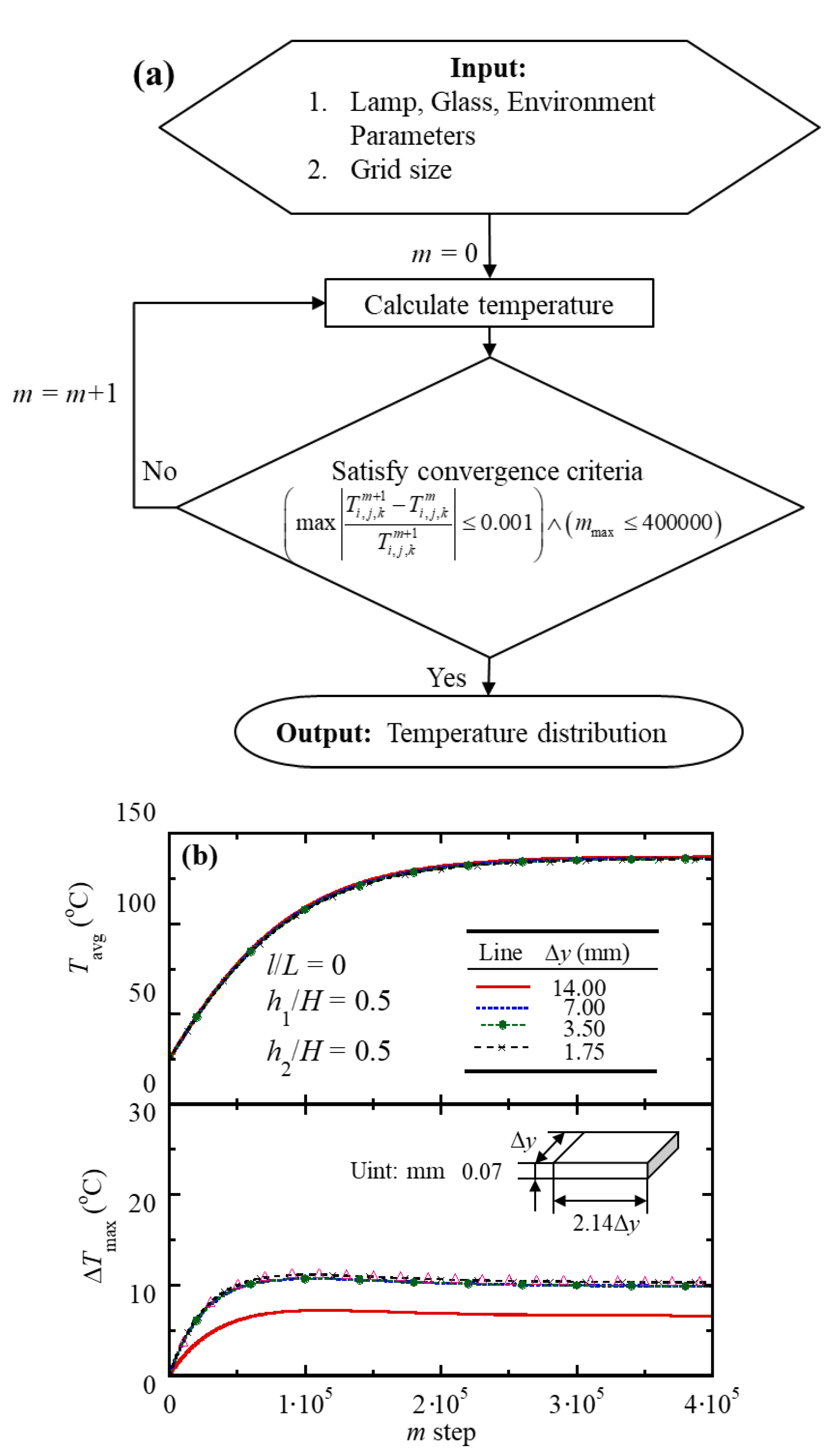
Figure 6.
Temperature distribution of a glass panel within different ovens. Subgraphs (a–c) are associated with l/L = 0, 1/6, and 1/3, respectively. Each subgraph contains nine distributions. Three in the same row are results corresponding to h1/H = 0.2, 0.5, and 0.8 from left to right. Three in the same column are results corresponding to h2/H = 0.2, 0.5, and 0.8 from top to bottom.


Figure 7.
Main effects of three control factors on Tavg and ΔTmax. Three subgraphs from top to bottom show the main effects of l/L, h1/H, and h2/H.
Figure 7.
Main effects of three control factors on Tavg and ΔTmax. Three subgraphs from top to bottom show the main effects of l/L, h1/H, and h2/H.


Table 1.
Three levels of control factors l/L, h1/H, and h2/H.
| Factor | Level 1 | Level 2 | Level 3 |
|---|---|---|---|
| l/L | 0 | 1/6 | 1/3 |
| h1/H | 0.2 | 0.5 | 0.8 |
| h2/H | 0.2 | 0.5 | 0.8 |
Table 2.
Average temperature Tavg (°C), maximum temperature difference ΔTmax (°C), and fitness function Q in all tests. Each test used an oven configuration specified with levels in the same row.
Table 2.
Average temperature Tavg (°C), maximum temperature difference ΔTmax (°C), and fitness function Q in all tests. Each test used an oven configuration specified with levels in the same row.
| Test | l/L (Level) | h1/H (Level) | h2/H (Level) | Tavg | ΔTmax | Q |
|---|---|---|---|---|---|---|
| 1 | 1 | 1 | 1 | 170.2 | 40.9 | 0 |
| 2 | 1 | 1 | 2 | 149.1 | 61.2 | 0 |
| 3 | 1 | 1 | 3 | 134.9 | 82.5 | 0 |
| 4 | 1 | 2 | 1 | 151.0 | 73.0 | 0 |
| 5 | 1 | 2 | 2 | 130.3 | 10.6 | 9.93 |
| 6 | 1 | 2 | 3 | 115.4 | 18.4 | 4.91 |
| 7 | 1 | 3 | 1 | 137.3 | 93.2 | 0 |
| 8 | 1 | 3 | 2 | 115.7 | 29.1 | 0 |
| 9 | 1 | 3 | 3 | 99.6 | 7.7 | 9.69 |
| 10 | 2 | 1 | 1 | 201.5 | 34.8 | 0 |
| 11 | 2 | 1 | 2 | 185.1 | 47.2 | 0 |
| 12 | 2 | 1 | 3 | 174.4 | 61.1 | 0 |
| 13 | 2 | 2 | 1 | 164.6 | 84.4 | 0 |
| 14 | 2 | 2 | 2 | 146.5 | 27.3 | 0 |
| 15 | 2 | 2 | 3 | 133.5 | 11.2 | 9.69 |
| 16 | 2 | 3 | 1 | 144.2 | 97.9 | 0 |
| 17 | 2 | 3 | 2 | 123.9 | 36.7 | 0 |
| 18 | 2 | 3 | 3 | 108.8 | 16.7 | 5.02 |
| 19 | 3 | 1 | 1 | 199.4 | 138.5 | 0 |
| 20 | 3 | 1 | 2 | 187.8 | 98.3 | 0 |
| 21 | 3 | 1 | 3 | 155.4 | 89.2 | 0 |
| 22 | 3 | 2 | 1 | 169.3 | 115.0 | 0 |
| 23 | 3 | 2 | 2 | 153.4 | 63.4 | 0 |
| 24 | 3 | 2 | 3 | 141.6 | 78.0 | 0 |
| 25 | 3 | 3 | 1 | 148.0 | 106.5 | 0 |
| 26 | 3 | 3 | 2 | 128.9 | 47.8 | 0 |
| 27 | 3 | 3 | 3 | 114.5 | 29.3 | 0 |
© 2018 by the authors. Licensee MDPI, Basel, Switzerland. This article is an open access article distributed under the terms and conditions of the Creative Commons Attribution (CC BY) license (http://creativecommons.org/licenses/by/4.0/).
Share and Cite
MDPI and ACS Style
Gu, M.-J.; Yang, S.; Wu, Y.-C.; Chiu, C.-J.; Chen, Y.-B. Designing a Thermal Radiation Oven for Smart Phone Panels. Inventions 2018, 3, 36. https://doi.org/10.3390/inventions3020036
AMA Style
Gu M-J, Yang S, Wu Y-C, Chiu C-J, Chen Y-B. Designing a Thermal Radiation Oven for Smart Phone Panels. Inventions. 2018; 3(2):36. https://doi.org/10.3390/inventions3020036
Chicago/Turabian StyleGu, Min-Jhong, Shuai Yang, Yen-Cheng Wu, Chien-Jui Chiu, and Yu-Bin Chen. 2018. "Designing a Thermal Radiation Oven for Smart Phone Panels" Inventions 3, no. 2: 36. https://doi.org/10.3390/inventions3020036