A New Observer Design for Fuzzy Bilinear Systems with Unknown Inputs

1
Department of Electrical Engineering and Electronics, Aoyama Gakuin University, Sagamihara 252-5258, Japan
2
Department of Mechanical and Aerospace Engineering, University of California, Los Angeles, CA 90095, USA
†
Current address: 420 Westwood Plaza, Los Angeles, CA 90095, USA.
Designs 2017, 1(2), 10; https://doi.org/10.3390/designs1020010
Submission received: 3 September 2017
/
Revised: 16 November 2017
/
Accepted: 16 November 2017
/
Published: 21 November 2017
(This article belongs to the Special Issue Optimization, Health Monitoring and Control Methods for Modern Complex Systems)
Abstract
:An observer design for a class of nonlinear systems with unknown inputs is considered. Takagi–Sugeno fuzzy bilinear systems represent a wide class of nonlinear systems, and these systems with unknown inputs are an ideal model for many physical systems. For such systems, a design method for obtaining an observer that estimates the state of the system is proposed. A parallel distributed observer (PDO), which is constructed with local linear observers and the appropriate grade of the membership functions, is a conventional observer for Takagi–Sugeno fuzzy bilinear systems. However, it is known that its design conditions have conservativeness. In this paper, to reduce the conservatism in the design conditions, non-PDO with new design conditions is proposed. Our design conditions are derived from a multiple Lyapunov function, which depends on the membership function with time-delay in the premise variables. This method eventually reduces the conservatism and enables us to construct an observer for a wide class of nonlinear systems. When the premise variables are the state variables that are not measurable, Takagi–Sugeno fuzzy bilinear systems can represent a wider class of nonlinear systems. Hence, an observer design for fuzzy bilinear systems with unmeasurable premise variables is also proposed. Finally, numerical examples are given to illustrate our design methods.
1. Introduction
It is well known that the Takagi–Sugeno fuzzy system has a great potential to describe a wide class of nonlinear systems [1]. It is a nonlinear system described by a set of fuzzy if-then rules that gives a local representation of an underlying system. Due to its importance, system analysis and control design based on Takagi–Sugeno fuzzy systems have been active (see [2,3,4,5,6] for example). As an extension of system representation, much attention has recently been paid to fuzzy bilinear systems. A bilinear system is a class of nonlinear systems, and its analysis and synthesis are of importance. Although both the fuzzy bilinear system and standard fuzzy system can describe nonlinear systems, a fuzzy bilinear system has the advantage of its representation with a lesser number of subsystems, which significantly reduces the conservatism in analysis and synthesis [7]. Due to its significant advantage, control problems for fuzzy bilinear systems have been considered, and many results have been given in [8,9,10,11,12,13,14,15,16]. For a controller design of fuzzy systems, a parallel distributed compensator (PDC) with a common Lyapunov function approach is conventionally employed. A PDC uses linear controllers corresponding to local linear systems, and a common Lyapunov function guarantees the stabilization. This method eventually produces the conservatism because a common Lyapunov function is exactly the same quadratic Lyapunov function for linear systems, despite the fact that a fuzzy system is nonlinear. To overcome this issue, a multiple Lyapunov function approach has been introduced in [4] where a descriptor system approach and multiple Lyapunov function were adopted. The descriptor approach reduced the conservatism in control design conditions for the state feedback control design. Although the analysis of descriptor systems is more complicated than state-space systems, they have richer structures that give less conservatism in the control design conditions. The multiple Lyapunov matrix method in [4] is a generalization of a common Lyapunov matrix method. However, this method requires the upper bound of the derivatives of the membership functions. The membership functions are not always differentiable, and their upper bounds are not easily calculated in advance. The recent papers [17,18] proposed the control design method based on a new multiple Lyapunov function approach. Since their Lyapunov function has an integral of the membership functions, any information on the derivatives of the membership functions is not necessary. Furthermore, their methods reduced the conservatism in the stability and control design for fuzzy systems.
Parallel to control design problems, a study on observer design for fuzzy systems has started [3,19,20,21,22,23,24]. An observer design for fuzzy bilinear systems has also been considered in [25,26,27,28], some of which are concerned with the design of an observer that attenuates unknown inputs. A conventional method of constructing an observer for a fuzzy system is based on a parallel distributed observer (PDO). Each sub-observer of a PDO corresponds to a local linear subsystem in a fuzzy system, and then, the overall fuzzy observer is constructed with the grade of the same membership functions for the system. Similar to control design, however, this approach is also found to be conservative because its design conditions stem from a common Lyapunov function. In the literature, a PDO has been extensively employed for fuzzy bilinear systems. A generalization of the PDO observer design is necessary. Another issue for the observer design of fuzzy systems is the availability of the premise variables. The premise variable plays an important role in the observer design for fuzzy systems. When the premise variable is the output, a fuzzy system representation is limited, but its observer design is simple because the premise variable can be used for the observer. When the premise variable is the state of the system, a fuzzy system describes a wider class of nonlinear systems, but its observer design becomes complicated because the premise variable is not available for the observer. The output feedback control and observer design with the unmeasurable premise variables was first considered in [29]. Since then, various methods of control and observer design have been proposed [22,23,30,31,32,33,34,35].
In this paper, we consider an observer design for nonlinear systems based on Takagi–Sugeno fuzzy bilinear models. First, we assume a new class of fuzzy observers and consider the stability of the error between the actual state and its estimate. In order to obtain less conservative stability conditions for the error system, we introduce a new type of multiple Lyapunov function. A multiple Lyapunov function is a natural extension of a common Lyapunov function. However, a conventional multiple Lyapunov function contains the membership function, and hence, the resulting stability condition depends on the derivative of the membership function, which is a function of the premise variable. This causes the issues that the membership function may not always be known a priori nor differentiable. In these cases, this design method is infeasible. Followed by [17,18], a class of multiple Lyapunov functions that contain an integral of the membership function of fuzzy systems is adopted. This approach requires no information on the derivative of the membership function and is shown to reduce the conservatism in control design conditions. Our multiple Lyapunov function eventually does not require the upper bound of the derivative of the membership function. Based on such a multiple Lyapunov function, an observer design method of fuzzy bilinear systems is proposed. Our observer design not only takes care of unknown inputs in the systems, but also fuzzy systems with the unmeasurable premise variables. The design methods for these extensions are also proposed. Finally, numerical examples are shown to illustrate our observer design method and to show the effectiveness of our approach.
2. Fuzzy Bilinear Systems
In this section, we introduce Takagi–Sugeno fuzzy bilinear systems. Consider the Takagi–Sugeno fuzzy model, described by the following IF-THENrules:
where is the state, is the control input, is the unknown input and is the measurement output. The matrices and C are constant matrices of appropriate dimensions, and C is of column full rank. r is the number of IF-THEN rules. are fuzzy sets, and , ⋯, are premise variables. We set . The premise variable is assumed to be measurable.
Then, the state and output equations are described by:
where:
and is the grade of the membership function of . We assume:
for any . Hence, satisfies:
for any .
Remark 1.
The standard Takagi–Sugeno fuzzy system can represent a nonlinear system. However, the Takagi–Sugeno fuzzy bilinear system has some advantages in estimation for nonlinear systems over the standard one. For example, consider the nonlinear system:
By a simple calculation, it can be written as the standard Takagi–Sugeno fuzzy system with :
The system can also be written as the Takagi–Sugeno fuzzy bilinear system with :
The system (4) can be written by (5) and (6) where is the membership function. The system (6) allows bilinear terms but the system (5) does not. The system (5) has four subsystems, while the system (6) has only two of these. This makes a big difference in analysis and synthesis. As we see in the literature, control and observer design conditions depend on the number of subsystems. The greater the number of subsystems a fuzzy system has, the more conservative the resulting design conditions are. Therefore, the number of subsystems is important, and establishment of observer design methods based on fuzzy bilinear systems gives an alternative approach to nonlinear systems.
Our problem is to find an observer that estimates the state of the system (1) and (2) and gets rid of unknown inputs in the system.
The following lemmas are given to prove our main results in the later sections.
Lemma 1.
Lemma 2.
([37]) Let and Q be matrices of appropriate dimensions. The following inequalities are equivalent.
- 1.
- A and are given. There exists such that:
- 2.
- A and are given. There exist and R such that:
Lemma 3.
([38]) Let and . If is a differentiable function on , then there exists a vector with such that:
where , and means the open interval between and .
Lemma 4.
([39]) For any given matrices of appropriate dimensions and scalar , we have:
3. Observer Design
In this section, we attempt to make an observer design. We first give stability conditions of the error system, and then, we propose a design method of observers for the fuzzy bilinear system (1) and (2). We also consider the generalization of the nonlinear output equation and unmeasurable premise variables.
3.1. Non-PDO Design
In the conventional observer design, the parallel distributed observer is usually employed. However, observer design conditions in this case are conservative. In order to avoid such conservatism, we adopt the non-parallel distributed observer (non-PDO). Let us assume the full-order observer of the form:
where is the vector and is the estimated state of . The matrices and are constant matrices of appropriate dimensions to be determined, and the variable is defined by:
for some scalar . We note that and:
which implies that and share the same properties as seen in (3).
Now, we state the first main result.
Theorem 1.
For a given , (7) and (8) become an observer for the system (1) and (2) if there exist matrices and T such that:
In this case, observer gains are calculated as:
where is a pseudoinverse matrix of C.
Proof.
We consider the error between the actual state and its estimate, which is defined by:
where:
Then, the error follows the dynamics:
If the following conditions are satisfied:
the error dynamics becomes:
Hence, if the system (25) is asymptotically stable, (7) and (8) become an observer for the system (1) and (2) under the conditions (21)–(24).
Let us obtain conditions for (25) to be asymptotically stable. To begin with, we consider a polytopic matrix:
The time-derivative can be calculated as:
where:
Taking into account, we consider the following Lyapunov function:
where are positive definite matrices to be determined. We calculate the time-derivative of to get:
Conditions (10)–(12) are not strict Linear Matrix Inequalities (LMIs), and (13) is a constraint. Due to this difficulty, we propose the following algorithm:
| Algorithm 1: |
|
Remark 2.
Theorem 1 is a generalized result of the existing ones in the literature because the multiple Lyapunov function approach is used in Theorem 1 while the single Lyapunov function approach was applied to the existing results. Hence, the observer (7) and (8) is a generalization of the PDO. As is readily seen, the observer (7) and (8) reduces to the PDO if . Multiple Lyapunov matrices obviously allow a wider region of solutions of the observer design conditions (10)–(13). The observer (7) and (8) and its multiple Lyapunov function also adopt the integral of the membership function, as well as its time delay function, which help (1) reduce the conservatism in the observer design conditions (10)–(13) and (2) avoid the derivatives of the membership functions in the observer design [17,18]. The knowledge of the derivative of the membership function is a tight requirement because the membership functions are not always differentiable and may not be calculated in advance. The existing results for the observer design of fuzzy bilinear systems employs the common Lyapunov function approach only and has never been extended to the use of the multiple Lyapunov function approach.
Remark 3.
Theorem 1 adopts Lemma 1 for the relaxation of its design condition. It is known [17] that although more decision variables are needed, Lemma 2 can make further relaxation of the conditions of Theorem 1. In fact, it follows from Lemma 2 and (30) that the condition (12) in Theorem 1 can be replaced by:
where and are matrices of appropriate dimensions, as well as and , to be chosen. This approach leads to less conservative results.
Letting and in Theorem 1, we have the following corollary as a special case of Theorem 1. Corollary 1 is basically equivalent to the result in [26], which proposes a design method for a conventional PDO.
Corollary 1.
In this case, observer gains are calculated as:
Proof.
If , then the condition (10) reduces to:
Letting leads to a reduction of the number of decision variables while preserving the advantages of this approach and, hence, reduces computational burden.
3.2. Generalization of the Nonlinear Output Equation
In the previous section, we assumed to have the linear output equation. However, it is more realistic that the output equation is nonlinear. Now, the output equation is given by:
For this generalization, we assume the following.
Assumption 1.
The following conditions are satisfied.
- 1.
- ;
- 2.
- is measurable.
Following the idea of [31], we shall transform the system (1) and (45) into the one without unknown input . It follows from (1) and (45) that:
The Assumption 1 allows us to obtain the unique solution:
where denotes the Moore–Penrose pseudoinverse of . In fact, is given by:
Despite the structures of and , using the sector nonlinearity technique [40], we can obtain the equivalent system described by the Takagi–Sugeno fuzzy system:
and (45) where satisfies:
Example 1.
Now, we have the system (48) and (45) without unknown input , and the corresponding observer to be proposed is assumed to be:
Theorem 2.
For a given , (49) becomes an observer for the system (48) and (45) if there exist matrices and such that:
In this case, observer gain is chosen such that:
Proof.
The error dynamics satisfies:
If the following conditions are satisfied:
the error dynamics becomes:
where:
Remark 4.
The transformation method in this section takes care of the nonlinear output equation. The nonlinear output equation is a generalization of not only the theoretical point of view, but also the practical point of view. It also eliminates the unknown input . This leads to no consideration of the unknown input in the observer design. It is a advantage to reduce the conservatism in the design conditions.
3.3. Extension to Observer Design with Unmeasurable Premise Variables
In Takagi–Sugeno fuzzy system representation, the premise variables play an important role. The premise variables basically describe nonlinearity in the system, but they are not always measurable variables. In order to design an observer for fuzzy systems with unmeasurable premise variables, we need to calculate the estimate of the unmeasurable premise variables.
For the case of the unmeasurable premise variables, we make the following assumptions:
Assumption 2.
The following conditions are satisfied.
- 1.
- 2.
For the system (1) and (2) with the unmeasurable premise variables, the following observer is proposed.
where is the estimate of . The error satisfies:
where:
Since , we have the identity:
where and are some constant matrices of appropriate dimensions. Applying Lemma 3 to (69), we find that there exists such that:
where . Applying Lemma 3 to in (63), assuming the linear transformation of where V is a constant matrix of appropriate dimension and adding (70), we obtain:
where:
Then, we have:
which implies that there exists a bound of the uncertainty . Now, we are in a position to give the following result.
Theorem 3.
Suppose that Assumption 2 holds. For a given and , (60) and (61) become an observer for the system (1) and (2) in the domain if there exist matrices and scalars such that:
where indicates the transpose of the off-diagonal block matrix. In this case, observer gains are calculated as:
where is a pseudoinverse matrix of C.
Proof.
We use the Lyapunov function (26) with replaced by and calculate the time-derivative of along the solution of (81) by applying Lemma 4 to get:
Making the same argument in (28) and applying the Schur complement formula, we see that:
is a sufficient condition for the system (81) to be asymptotically stable in the domain . Rewriting (83) as:
and applying Lemma 1, we get (72)–(74), and (75) follows from (67). Gains follow from (19), (28), (29), (64)–(66). This completes the proof. ☐
Remark 5.
If there is no difference between and , then Δ becomes zero. This implies that we can take in (74) and consequently can choose big enough for (74) to be satisfied. This means the conditions in Theorem 3 reduce to those in Theorem 1. Algorithm 1 may be used to solve the design conditions (72)–(75). Alternatively, for the case of the nonlinear output equation and elimination of the unknown input term, the technique in Section 3.2 is applicable to the observer design with the unmeasurable premise variables.
Remark 6.
For the reduction of the computational burden, simplification of and can be applied to Theorems 2 and 3, respectively, as we obtain Corollary 2.
4. Numerical Examples
We consider three examples here. Example 2 compares our main design method with the existing method. Example 3 shows the observer design with the unmeasurable premise variables. Finally, Example 4 takes care of the practical system for two cases of the linear and nonlinear measurement output equations.
Example 2.
Consider the fuzzy bilinear system (1) and (2) with the following system matrices:
and the membership functions are given by:
For this system, none of the conditions of Corollary 1, Theorem 3.1 in [41], Theorem 1 in [26] and Theorem 1 in [27] are satisfied, and hence, these results do not make an observer design. In order to compare with Theorem 2 in [42] and Theorem 1 in [43], we let (because [42] only considers the standard fuzzy system). Conditions of Theorem 2 in [42] and Theorem 1 in [43] fail to be satisfied. On the other hand, Theorem 1 and Corollary 2 allow us to design an observer. This implies that Theorem 1 and Corollary 2 comprise a less conservative observer design method. Other results including Corollary 1 are based on a conventional PDO approach with the common Lyapunov matrix. In fact, Theorem 1 allows us to construct the observer (7) and (8) with:
Example 3.
We consider a nonlinear system described by:
For and , this system can be written as the system (1)–(2) with the following matrices:
and the membership functions:
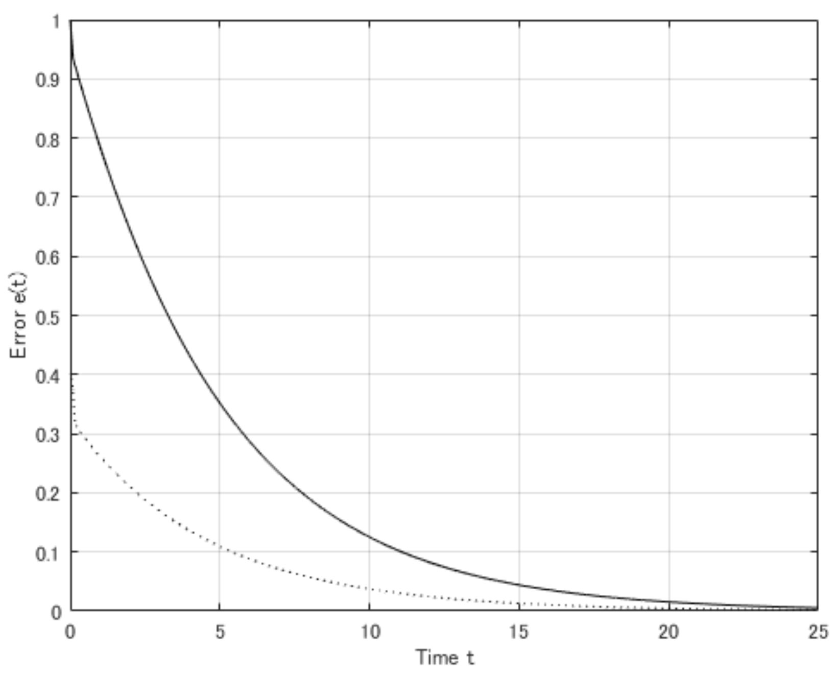
The premise variable for this system is , which is not measurable. Hence, we shall design an observer (60) and (61) with the unmeasurable premise variable. The error of the immeasurable premise variable . and . It follows that . Assume that . Then, we calculate . Observer gain matrices can be calculated by Theorem 3 as:
Given the initial conditions , the simulation result is shown in Figure 1. The solid line and dotted line indicate the errors and , respectively. The designed observer obviously estimates the true values of the states and since the errors and converge to zero.
Example 4.
We shall design an observer for an isothermal continuous stirred tank reactor (CSTR) [41,44], whose dynamics can be described by:
where the state represents the concentration of the reactant inside the reactor (mol/L) and the state is the concentration of the product in the CSTR output stream (mol/L). The input-feed stream to the CSTR consists of a reactant with concentration , and the controlled input is the dilution rate where F is the input flow rate to the reactor (L/h) and V is the constant volume of the CSTR (L). The kinetic parameters are chosen to be and as in [44]. We assume that . The system (84) can be written into (1) and (2) with the following matrices:
with the membership functions:
For a finite value , we can design a local observer, and for , we can construct a global observer. The output determines the grade of the final product and is assumed to be the following two cases.
Case 1: The output equation is linear:
It is shown in [41] that for , an observer can be designed. However, ; the method in [41] fails to design an observer. Even for , Theorem 1 still guarantees the designing of an observer. This concludes that Theorem 1 guarantees a much wider stability region of the error system.
Case 2: The output equation is nonlinear:
Applying the technique in Section 3.2, we transform the system (84) into:
which, under the assumption that , can be written as (45) and (48) with:
Defining , we have the membership functions:
Let . Theorem 2 designs the observer (49) with the membership functions (85). Note that we can calculate from the output equation where is the measurable output. Solving for , we get:
uniquely for . Given the initial conditions , the simulation result is shown in Figure 2. The solid line and dotted line indicate the error and , respectively. The designed observer obviously works well, as wee see the error and converge to zero.
5. Conclusions
An observer design method for Takagi–Sugeno fuzzy bilinear systems with unknown inputs has been proposed. A non-PDO was introduced, and new design conditions based on a multiple Lyapunov function were given. This approach reduces the conservatism of observer design and allows us to construct an observer for a wide class of nonlinear systems. The generalization of the nonlinear output equation and the observer design method with the unmeasurable premise variables were also considered. Finally, numerical examples were given to illustrate our results.
Acknowledgments
This work is supported by JSPS KAKENHI Grant Number 26330283.
Conflicts of Interest
The author declares no conflict of interest. The founding sponsors had no role in the design of the study; in the collection, analyses, or interpretation of data; in the writing of the manuscript, and in the decision to publish the results.
References
- Takagi, T.; Sugeno, M. Fuzzy identification of systems and its applications to modeling and control. IEEE Trans. Syst. Man Cybern. 1985, 15, 116–132. [Google Scholar] [CrossRef]
- Dong, S.; Wu, Z.-G.; Shi, P.; Su, H.; Lu, R. Reliable control of fuzzy systems with quantization and switched actuator failures. IEEE Trans. Syst. Man Cybern. Syst. 2017, 47, 2198–2208. [Google Scholar] [CrossRef]
- Lendek, Z.; Guerra, T.M.; Babuska, R.; De Schutter, B. Stability Analysis and Nonlinear Observer Design Using Takagi–Sugeno Fuzzy Models; Springer: Berlin, Germany, 2010. [Google Scholar]
- Tanaka, K.; Ohtake, H.; Wang, H.O. A descriptor system approach to fuzzy control system design via fuzzy Lyapunov functions. IEEE Trans. Fuzzy Syst. 2007, 15, 333–341. [Google Scholar] [CrossRef]
- Tanaka, K.; Sugeno, M. Stability analysis and design of fuzzy control systems. Fuzzy Sets Syst. 1992, 45, 135–156. [Google Scholar] [CrossRef]
- Wu, Z.-G.; Dong, S.; Shi, P.; Su, H.; Huang, T.; Lu, R. Fuzzy-model-based non fragile guaranteed cost control of nonlinear Markov jump systems. IEEE Trans. Syst. Man Cybern. Syst. 2017, 47, 2388–2397. [Google Scholar] [CrossRef]
- Yoneyama, J. Nonlinear control design based on generalized Takagi–Sugeno fuzzy systems. J. Frankl. Inst. 2014, 351, 3524–3535. [Google Scholar] [CrossRef]
- Gao, Z.-F.; Chen, J.; Liu, F. Guaranteed cost control for fuzzy bilinear systems with uncertain parameters. In Proceedings of the 2010 International Conference on Electrical Engineering, Computing Science and Automatic Control, Tuxtla Gutierrez, Mexico, 8–10 September 2010; pp. 644–647. [Google Scholar]
- Guo, Z.; Bo, R. Non-fragile static output controller design for fuzzy systems. In Proceedings of the 2000 International Conference on Intelligent System Design and Engineering Application, Changsha, China, 13–14 October 2010; pp. 1017–1020. [Google Scholar]
- Li, T.-H.S.; Tsai, S.-H.; Lee, J.-Z.; Hsiao, M.-Y.; Chao, C.-H. Robust H∞ fuzzy control for a class of uncertain discrete fuzzy nonlinear systems. IEEE Trans. Syst. Man Cybern. Part B 2007, 38, 510–527. [Google Scholar] [CrossRef] [PubMed]
- Li, T.-H.S.; Tsai, S.-H. T–S fuzzy bilinear model and fuzzy controller design for a class of nonlinear systems. IEEE Trans. Fuzzy Syst. 2007, 15, 494–506. [Google Scholar] [CrossRef]
- Takada, R.; Uchida, Y.; Yoneyama, J. Output Feedback Stabilization of Takagi–Sugeno Fuzzy Bilinear Time-Delay Systems. In Proceedings of the 2012 IEEE International Conference on Fuzzy Systems, Brisbane, Australia, 10–15 June 2012; pp. 300–307. [Google Scholar]
- Takada, R.; Uchida, Y.; Yoneyama, J. Output feedback guaranteed cost control for fuzzy bilinear systems. Appl. Math. Sci. 2013, 7, 1303–1318. [Google Scholar]
- Tsai, S.-H.; Li, T.-H.S. Robust fuzzy control of a class of fuzzy bilinear systems with time-delay. Chaos Solitons Fractals 2009, 39, 2028–2040. [Google Scholar] [CrossRef]
- Yoneyama, J. Stabilization of Takagi–Sugeno fuzzy bilinear time-delay systems. In Proceedings of the 2010 IEEE Multi-Conference Systems and Control, Yokohama, Japan, 8–10 September 2010; pp. 111–116. [Google Scholar]
- Yoneyama, J. Output feedback control design for Takagi–Sugeno fuzzy bilinear time-delay systems. In Proceedings of the 2010 IEEE Conference on Systems, Man and Cybernetics, Istanbul, Turkey, 10–13 October 2010; pp. 1671–1677. [Google Scholar]
- Marquez, R.; Guerra, T.M.; Bernal, M.; Kruszewski, A. A non-quadratic Lyapunov functional for H∞ control of nonlinear systems via Takagi–Sugeno models. J. Frankl. Inst. 2016, 353, 781–796. [Google Scholar] [CrossRef]
- Yoneyama, J.; Hoshino, K. A novel non-fragile output feedback controller design for uncertain Takagi–Sugeno fuzzy systems. In Proceedings of the World Congress on Computational Intelligence, Vancouver, BC, Canada, 24–29 July 2016; pp. 2193–2198. [Google Scholar]
- Estrada-Manzo, V.; Guerra, T.M.; Lendek, Z. An LMI approach for observer design for Takagi–Sugeno descriptor models. In Proceedings of the 2014 IEEE International Conference on Automation, Quality and Testing, Robotics, Cluj-Napoca, Romania, 22–24 May 2014. [Google Scholar]
- Shi, P.; Su, X.; Li, F. Dissipativity-based filtering for fuzzy switched systems with stochastic perturbation. IEEE Trans. Autom. Control 2016, 61, 1694–1699. [Google Scholar] [CrossRef]
- Shi, P.; Zhang, Y.; Chadli, M.; Agarwal, R.K. Mixed H-infinity and passive filtering for discrete fuzzy neural networks with stochastic jumps and time delays. IEEE Trans. Neural Netw. Learn. Syst. 2016, 27, 903–909. [Google Scholar] [CrossRef] [PubMed]
- Yoneyama, J. H∞ Filtering for Fuzzy Systems with Immeasurable Premise Variables: An Uncertain System Approach. Fuzzy Sets Syst. 2009, 160, 1738–1748. [Google Scholar] [CrossRef]
- Yoneyama, J. H∞ Filtering for Sampled-Data Systems. In Proceedings of the 2009 IEEE International Conference on Control and Automation, Christchurch, New Zealand, 9–11 December 2009; pp. 1728–1733. [Google Scholar]
- Yoneyama, J.; Nishikawa, M.; Katayama, H.; Ichikawa, A. Output stabilization of Takagi–Sugeno fuzzy systems. Fuzzy Sets Syst. 2000, 111, 253–266. [Google Scholar] [CrossRef]
- Saoudi, D.; Mechmeche, C.; Braiek, N.B. T-S fuzzy bilinear observer for a class of nonlinear systems. In Proceedings of the 18th Mediterranean Conference on Control and Automation, Marrakech, Morocco, 23–25 June 2010; pp. 1395–1400. [Google Scholar]
- Saoudi, D.; Chadli, M.; Braiek, N.B. State estimation of unknown input fuzzy bilinear systems: Application to fault diagnosis. In Proceedings of the 2013 European Control Conference, Zurich, Switzerland, 17–19 July 2013; pp. 2465–2470. [Google Scholar]
- Saoudi, D.; Chadli, M.; Braiek, N.B. Robust H∞ fault detection for fuzzy bilinear systems via unknown input observer. In Proceedings of the 22nd Mediterranean Conference on Control and Automation, Palermo, Italy, 16–19 June 2014; pp. 281–286. [Google Scholar]
- Tsai, T.H. A global exponential fuzzy observer design for time-delay Takagi–Sugeno uncertain discrete fuzzy bilinear systems with disturbance. IEEE Trans. Fuzzy Syst. 2012, 20, 1063–1075. [Google Scholar] [CrossRef]
- Yoneyama, J.; Nishikawa, M.; Katayama, H.; Ichikawa, A. Design of output feedback controllers for Takagi–Sugeno fuzzy systems. Fuzzy Sets Syst. 2001, 121, 127–148. [Google Scholar] [CrossRef]
- Guerra, T.M.; Marquez, R.; Kruszewski, A.; Bernal, M. H∞ LMI-based observer design for nonlinear systems via Takagi–Sugeno models with unmeasured premise variables. IEEE Trans. Fuzzy Syst. 2017, PP. [Google Scholar] [CrossRef]
- Rotondo, D.; Witczak, M.; Puig, V.; Nejjari, F.; Pazera, M. Robust unknown input observer for state and fault estimation in discrete-time Takagi–Sugeno systems. Int. J. Syst. Sci. 2016, 47, 3409–3424. [Google Scholar] [CrossRef] [Green Version]
- Wang, L.K.; Zhang, H.G.; Liu, X.D. H∞ observer design for continuous-time Takagi–Sugeno fuzzy model with unknown premise variables via nonquadratic Lyapunov function. IEEE Trans. Cybern. 2016, 46, 1986–1996. [Google Scholar] [CrossRef] [PubMed]
- Yoneyama, J.; Ishihara, T. Control Design of Fuzzy Systems with Immeasurable Premise Variables. In Fuzzy Systems; In-Tech: Rijeka, Croatia, 2010. [Google Scholar]
- Yoneyama, J. Robust H∞ Output Feedback Control for Uncertain Fuzzy Systems with Immeasurable Premise Variables. Adv. Fuzzy Sets Syst. 2008, 3, 99–113. [Google Scholar]
- Yoneyama, J. H∞ Output Feedback Control for Fuzzy Systems with Immeasurable Premise Variables: Discrete-Time Case. Appl. Soft Comput. 2008, 8, 949–958. [Google Scholar] [CrossRef]
- Tuan, H.D.; Apkarian, P.; Narikiyo, T.; Yamamoto, Y. Parameterized linear matrix inequality techniques in fuzzy control system design. IEEE Trans. Fuzzy Syst. 2001, 9, 324–332. [Google Scholar] [CrossRef]
- Peaucelle, D.; Arzelier, D.; Bachelier, O.; Bemussou, J. A new robust D-stabiity condition for real convex polytopic uncertainty. Syst. Control Lett. 2000, 40, 21–30. [Google Scholar] [CrossRef]
- Zill, D.G.; Wright, W.S. Calculus: Early Transcendentals; Jones & Bartlett Publishers: Burlington, MA, USA, 2010. [Google Scholar]
- Xie, L.; de Souza, C.E. Robust H∞ control for linear systems with norm-bounded time-varying uncertainty. IEEE Trans. Autom. Control 1992, 37, 1188–1191. [Google Scholar] [CrossRef]
- Tanaka, K.; Wang, H.O. Fuzzy Control Systems Design and Analysis: A Linear Matrix Inequality Approach; Wiley: Hoboken, NJ, USA, 2000. [Google Scholar]
- Saoudi, D.; Chadli, M.; Mechmeche, C.; Braiek, N.B. Unknown input observer design for fuzzy bilinear system: An LMI approach. Math. Probl. Eng. 2012, 2012, 794581. [Google Scholar] [CrossRef]
- Chadli, M.; Karimi, H.R. Robust observer design for unknown inputs Takagi–Sugeno models. IEEE Trans. Fuzzy Syst. 2013, 21, 158–164. [Google Scholar] [CrossRef]
- Li, S.; Wang, H.; Aitouche, A.; Tian, Y.; Christov, N. Robust unknown input observer design for state estimation and fault detection using linear parameter varying model. J. Phys. Conf. Ser. 2017, 783, 012001. [Google Scholar] [CrossRef]
- Perez, H.; Ogunnaike, B.; Devasia, S. Output tracking between operating points for nonlinear processes: Van de Vusse example. IEEE Trans. Control Syst. Technol. 2002, 10, 611–617. [Google Scholar] [CrossRef]
Figure 1.
The error trajectories.
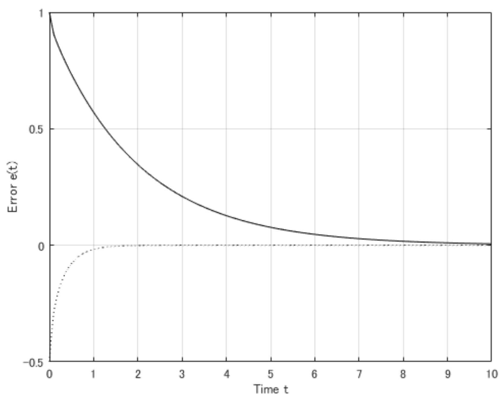
Figure 2.
The error trajectories.

© 2017 by the author. Licensee MDPI, Basel, Switzerland. This article is an open access article distributed under the terms and conditions of the Creative Commons Attribution (CC BY) license (http://creativecommons.org/licenses/by/4.0/).
Share and Cite
MDPI and ACS Style
Yoneyama, J. A New Observer Design for Fuzzy Bilinear Systems with Unknown Inputs. Designs 2017, 1, 10. https://doi.org/10.3390/designs1020010
AMA Style
Yoneyama J. A New Observer Design for Fuzzy Bilinear Systems with Unknown Inputs. Designs. 2017; 1(2):10. https://doi.org/10.3390/designs1020010
Chicago/Turabian StyleYoneyama, Jun. 2017. "A New Observer Design for Fuzzy Bilinear Systems with Unknown Inputs" Designs 1, no. 2: 10. https://doi.org/10.3390/designs1020010