Demand Response Design of Domestic Heat Pumps

Faculty of Engineering, University of Kufa, P.O. Box (21), Najaf Governorate, 54001 Al Najaf, Iraq
Designs 2018, 2(1), 1; https://doi.org/10.3390/designs2010001
Submission received: 23 November 2017
/
Revised: 14 December 2017
/
Accepted: 19 December 2017
/
Published: 23 December 2017
(This article belongs to the Special Issue Challenges and Progress in Turbomachinery Design)
Abstract
:This paper proposes an emergency-based demand response (DR) controller of domestic heat pump (DHP) units based on an estimated frequency of the UK electricity in 2035. The normal pattern of DHP demand is adjusted to maintain system frequency within its limit using a linear model of power and temperature inside low-carbon houses, while considering consumer comfort. Simulation results show that the proposed DR design of static/dynamic frequency-controlled DHPs will increase the amount of power reserve by 75% and the amount of electricity market by 70%, as compared to their values of the current frequency response by flexible loads.
1. Introduction
The residential sector of European countries forms nearly 40% of their overall energy consumption [1]. A reasonable level of economic and environmental objectives can be attained by adjusting some flexible domestic loads. Demand response (DR) schemes adapt the normal pattern of end-user power consumption using an external signal. The DR schemes are mainly classified into two types, which are emergency-based and economic-based designs. An emergency-based DR design adjusts end-user energy using direct load control (DLC) signals (e.g., system frequency), whereas an economic-based DR design adjusts end-user energy using price signals (e.g., time-of-use tariff) [2].
A dynamic demand control was studied in [3] to maintain system frequency using domestic appliances (refrigerators). The study of [3] demonstrated that the decline of system frequency could be delayed by controlling the demand side without a major contribution of backup generators. Centralized, decentralized, and hierarchical frameworks were discussed in [4] to achieve controllable electric loads, while providing ancillary services (e.g., contingency and regulation reserves). A decentralized DR approach was addressed in [5] to maintain system frequency without intensive communications between control and demand entities. Some demand-side management techniques were reviewed in [6], while simulating a specific DR strategy using heating, ventilating and air conditioning systems across a group of 629 residential buildings. Moreover, several DR programs were surveyed in [7] for sustainable energy systems, presenting different strategies of application and implementation in a smart grid paradigm.
1.1. Problem Description
The system operability framework (SOF) [8] examined the effect of future energy scenarios (FES) [9] on the UK power system. The operational challenges of UK power systems were estimated over the next two decades. It was concluded that both short circuit capacity and system inertia will decrease due to the integration of renewable energy sources (RES) [8]. Synchronous generators naturally contribute to the system inertia, which resists the change of system frequency when an event (e.g., plant outage) triggers frequency fluctuations [10]. However, RES nonsynchronous generators are connected to power systems using solid-state devices that have no inertia. National Grid has to maintain system frequency between 49.5–50.5 Hz. Maintaining system frequency within this limit will be a challenging issue beyond 2020 due to a subsequent reduction of system inertia with RES integration [8].
1.2. Potential Solution
A provider of ancillary services restores system frequency either traditionally using flexible electricity generators, or alternatively using a DR scheme. In this context, the DR scheme represents demand reduction using a high number of small-scale loads to provide an equivalent response from a backup electricity generator. National Grid uses different DR schemes to match supply with demand based on the following requirements of each DR service.
- Short term operating reserve (STOR) service is used in a form of demand reduction or backup generation. With a short notice of 4 h ahead, a STOR provider must supply at least 3 MW power over a minimum interval of 2 h [11]. The average payment of the STOR service was £25,000/MW per year in 2015/16 [12,13,14].
- Static frequency control by demand management (FCDM) service needs a minimum power of 3 MW over a half-hour time interval to deliver this service. System frequency triggers the FCDM service when it declines below 49.7 Hz [16]. The average payment of the FCDM service was £35,000/MW per year in 2015/16 [12,13,14].
1.3. Paper Contribution
This paper investigates two types of DR controllers, which are the dynamic and static controllers of domestic heat pump (DHP) units. The dynamic DR controller is implemented based on the FFR requirements, whereas the static DR controller is designed based on the FCDM requirements. In the dynamic DR controller, the available power reserve is regularly changing its amount, while responding to the rate of change of frequency. On the other hand, an aggregated power reserve is obtained in the static DR controller based on a threshold of system frequency. The proposed emergency-based DR controller requires a proper mathematical model of studied heating systems to provide such service. Therefore, the contributions of the paper are highlighted as follows.
- Developing a linear mathematical model of the DHPs in low-carbon domestic buildings.
- Managing power consumption of the DHPs based on a square root function of system frequency while considering climate-controlled temperature inside the buildings.
- Reporting the available DR reserve of the DHPs in advance.
- Estimating an average payment of such DR reserve.
1.4. Paper Structure
The rest of this paper is organized as follows. Mathematical models of system frequency and DHP unit are presented in Section 2. The proposed DR controller by load management is described in Section 3 based on the considerations of prediction, assumption, and implementation. Simulation results are shown in Section 4, while conclusions are given in Section 5.
2. Mathematical Models
System frequency and DHP unit are mathematically modelled in this study to evaluate the available DR reserve in advance.
2.1. System Frequency
Equation (1) is a square root function that calculates system frequency based on the total kinetic energy of rotating mass connected to the UK system [3].
where is the system frequency updated over successive time steps (i.e., ). is the width of each time step. is the nominal system frequency (i.e., Hz for the UK). is the difference between the overall power of generation and consumption. is the total kinetic energy of connected rotating mass to the system in GWs. According to [17], the relationship between the rate of change of frequency and power deviation is illustrated as follows:
where is the rate of change of frequency. Thus, the rate of change of frequency is predicted using the following equation:
where and are the present and predicted rate of change of frequency based on the same amount of power difference between generation and consumption (i.e., ). and are the current and future total kinetic energy of rotating mass connected to the system.
2.2. Domestic Heat Pump
The coefficient of performance () is used to calculate electricity demand of the DHPs. In fact, the () value represents the efficiency of heat transfer.
where are output and input power of the DHP unit in kW. The DHPs are used in conjunction with the thermal resistivity of buildings to maintain climate-controlled temperatures within comfortable conditions. Equation (5) is used to calculate electricity consumption by the DHPs [18].
where is the air density in kg/m3. is specific heat of air in kJ/kg°C. is the air flow rate in m3/s, which represents the measurement of a sensor that records the volume and density of the air entering heating engine to calculate the power required based on the model developed in the paper. is the difference between supply and return temperatures of the DHPs in °C. According to Carnot’s cycle, the efficiency of heating engine is calculated based on the difference of temperatures across that engine. Carnot’s equation is multiplied by a factor () to acquire realistic values of () for the DHPs. The factor in Equation (6) is empirically adjusted based on the literature [19,20] to determine the value of () as shown below.
where is a numerical constant (i.e., ) to convert temperature from Celsius scale into Kelvin scale. is the supply temperature of the DHP unit in °C. is the outdoor temperatures in °C. By substituting Equation (6) in (5), electricity power consumption is calculated as follows.
where is the rate of electricity power consumption in kW at the time step relative to variable outdoor temperatures (). Equation (8) is used to determine the rate of heat losses to outdoor environment through walls and fenestrations [21].
where is the rate of heat losses in kW at the time step considering the variable outdoor temperatures (i.e., ). is the return temperature of the DHP unit in °C. is the equivalent thermal resistivity of the walls and fenestrations in °C/kW. However, the wall capacitance was not considered (i.e., the limitation of the study). Therefore, the climate-controlled temperature () in °C is updated in every time step using the following equation.
where is the air mass flow in kg/s. The DHPs are equipped with load control devices (thermostats). The complete model of electricity demand is represented by considering thermostatic operational cycles of the DHP unit, as shown below.
where is the electricity demand of the DHP unit in kW at time step considering thermostat operations. is the off-state thermostatic temperature (i.e., 20 °C). Table 1 shows the considered parameters of the DHPs.
3. Emergency-Based Demand Response
The design of the emergency-based DR program requires highlighting the prediction, assumption, and implementation, which are considered in this study. Therefore, these considerations are systematically presented as follows.
3.1. Prediction
A number of DHPs are predicted over the coming years based on the FES by National Grid [9], as shown in Table 2. The low scenario in 2035 (i.e., 849,558 units in Table 2) is considered in this study. The distribution of the DHPs across the different zones of distribution network operator (DNO) is calculated based on the statistics of UK households for each geographical area, as presented in Table 3. These statistics are reported by office for gas and electricity market (Ofgem) [22].
3.2. Assumption
The following assumptions are considered to present the work of this study.
- The value of () is estimated to drop from the current amount of 360 GWs to just 150 GWs in the UK by 2035, as presented in [8].
- Daily ambient temperatures of January, February and December (2014) in the UK [23] were used to predict ambient temperatures on a winter day by 2035 using a normal probabilistic distribution. The winter was only considered because the DHP unit will be in a semi-idle state in UK residential dwellings during summer.
- The dynamic DR controller of the DHPs is activated based on a generation loss of 1.32 GW from the UK power system [24]. Meanwhile, the static DR controller is activated based on a normal probabilistic deviation between supply and demand with the mean value of 0 GW and standard deviation of 0.5 GW over a day.
- Each DNO is assumed to be responsible for providing the DLC signals that control the DHPs accordingly, using information and communication technologies (ICTs). In this context, aggregator is the technical term that should be used to call DNO entities.
- Domestic buildings were modelled considering the low-carbon houses of high-thermal mass materials, which indicate a slow decline of the internal temperature when the DHP is switched off over a short-term timescale [25].
- Equivalent thermal resistivity is synthesized using a uniform probabilistic distribution to represent a variety of modelled buildings. This consideration is identified based on an evaluation of heat losses through external walls and fenestrations [21].
3.3. Implementation
The DLC signal of the static DR controller is used to control the DHPs considering system frequency and climate-controlled temperature based on the following conditions.
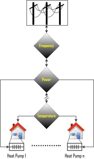
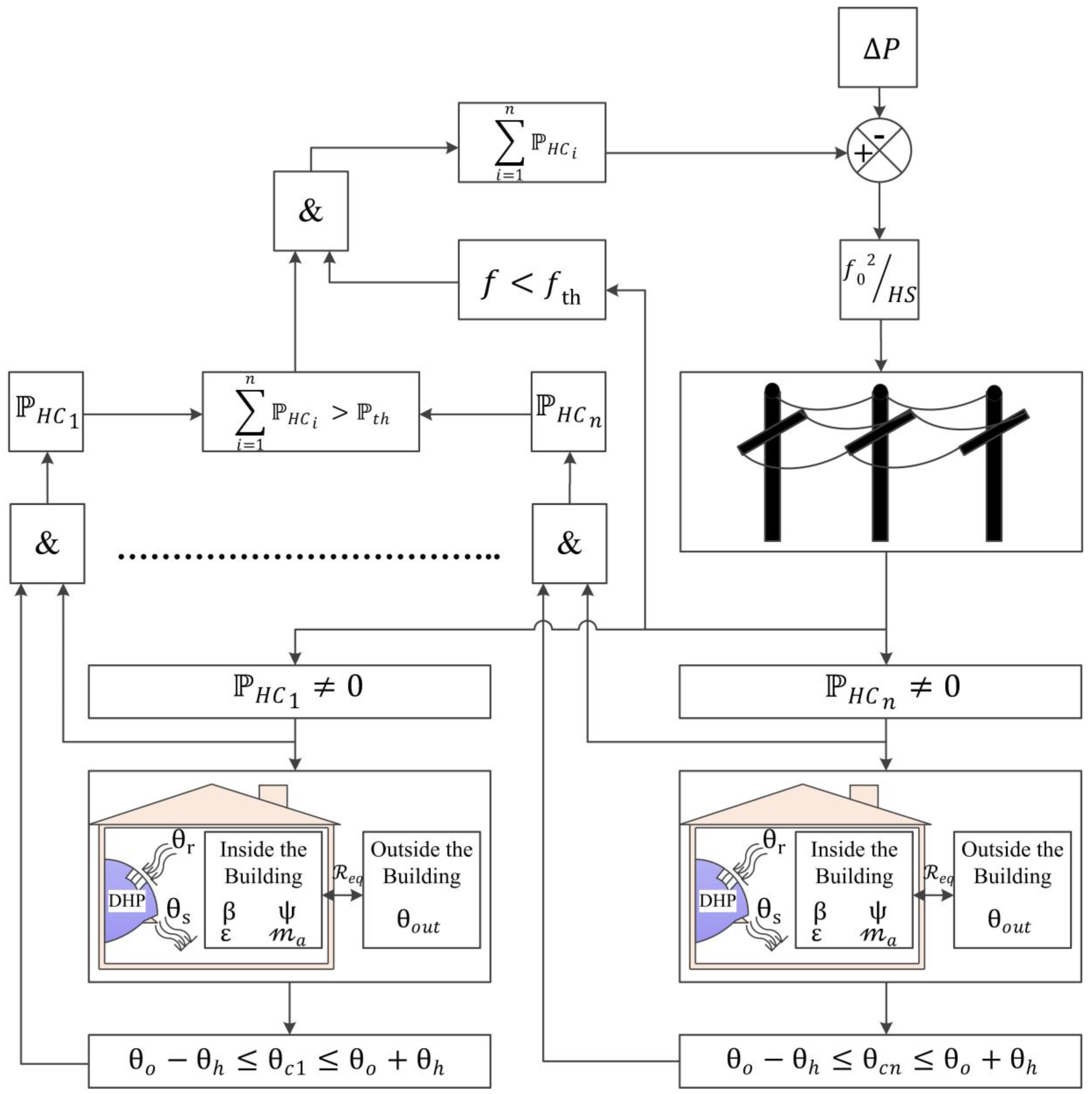
where is the total number of the DHPs for each DNO area. is the minimal power that is required to obtain the DR reserve ( MW). is the electricity demand of the DHPs in kW at time step considering frequency control and thermostat operation simultaneously. is the activation threshold of frequency ( Hz). is the range of the climate-controlled temperatures of the buildings based on a thermostatic hysteresis of 1 °C (i.e., ). is a real, integer and positive number. Figure 1 shows the proposed static DR controller using demand reduction of the DHPs in the UK domestic buildings. In the meantime, the dynamic DR controller is designed based on the rate of change of frequency (), considering a value of MW.
4. Simulation Results
By considering the parameters of Table 1, all DHPs were modelled on a 15-minute basis over a day. Figure 2a depicts the average value of daily ambient temperatures in 2035 considering the UK weather temperatures, as recorded in winter [23]. Figure 2b illustrates the internal temperature of a building modelled with a DHP unit. This temperature fluctuates around 20 °C based on thermal resistivity, thermal mass, ambient temperature and other factors, as evaluated in Section 2.2 and Section 3.2. Figure 2c demonstrates the electric loads of the DHPs, which are dependent on their coefficient of performance as shown in Figure 2d. Similarly, these characteristics were determined for all DHPs modelled in this paper.
Figure 3 shows the frequency of the values of and for the DHPs evaluated in DNO14. The numbers of the DHPs were considered for each DNO area based on Table 3.
Figure 3a indicates the recurrence of the thermal resistivity for the buildings modelled at the zone of DNO 14. It can be seen that the values of the thermal resistivity vary within a bounded room of a uniform probabilistic distribution, as considered in Section 3.2. Figure 3b illustrates the frequency of the coefficient of performance for the DHPs considered at the area of DNO 14. Figure 3c shows the recurrence of the daily climate-controlled temperatures for the buildings investigated at the region of DNO 14. Figure 3d depicts the frequency of the daily electricity loads of the DHPs considering their number in DNO 14, as shown in Table 3.
Figure 4 demonstrates the overall electricity demand of the DHPs predicted for each DNO area by 2035. For example, the overall electricity demand is calculated in DNO1 by aggregating the electricity loads of 25,487 DHPs over a day considering the UK weather in winter.
According to West Midlands Public Health Observatory (UK), “an adequate level of wintertime warmth is 21 °C (70 °F) for a living room, and a minimum of 18 °C (64 °F) for other occupied rooms, giving 24 °C (75 °F) as a maximum comfortable room [i.e., climate-controlled] temperature for sedentary adults”. Thus, the DR reserve is only provided with the buildings that have a climate-controlled temperature between 19 °C and 21 °C to maintain a convenient use of the DHPs.
Figure 5 shows an estimate of the total electricity demand for each DNO area based on the conditions of Equation (11). When the system frequency declines below the threshold, a load shedding of frequency-controlled DHPs will be activated considering the limited range of comfortable internal temperatures (i.e., between 19–21 °C). The proposed design of frequency-controlled DHP is able to maintain consumer comfort while supplying the dynamic/static DR reserve based on the following criteria:
- Thermal mass of low-carbon buildings.
- Thermal resistivity of these buildings.
- Demand diversity across DNO areas.
Figure 6 represents system frequency using the proposed design of dynamic DR controller taking into account the present and predicted values of the UK total kinetic energy, as mentioned in [8]. The system frequency is evaluated in Figure 6 considering three different scenarios of the 1.32 GW of generation loss in the UK electricity system. Two scenarios were determined using 360 GWs and 150 GWs of without the DR design of frequency-controlled DHPs. Meanwhile, the third scenario is calculated based on the 150 GWs of while considering 1.05 GW load shedding of frequency-controlled DHPs in all DNO areas. The 1.05 GW power reserve is estimated based on Figure 4 because the dynamic frequency-controlled DHPs will be requested over a 30 s only.
Figure 7 shows the comparison between daily system frequency with and without the DR reserve of frequency-controlled DHPs. The static power reserve is obtained by aggregating the power of frequency-controlled DHPs at DNO9 as it can provide a sufficient power reserve for such drop in system frequency. If there is a further decline of system frequency, more power reserve can be supplied by load shedding of extra frequency-controlled DHPs considering other DNO areas.
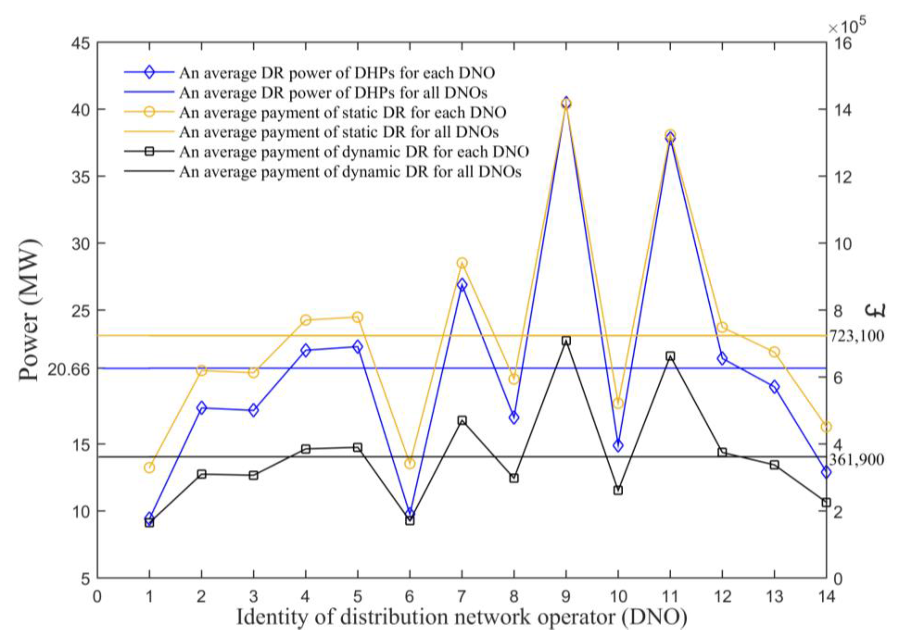
Figure 8 illustrates power share of electricity demand reduction for each DNO area using these DHPs, differentiating DNO9 as it provides the higher power reserve. Figure 9 gives an estimate of the total payment with the proposed DR controller for each DNO zone, considering the current DR market (i.e., reported in [12,13,14]). The average power reserve for each DNO region using the DHPs is also illustrated in Figure 9. Table 4 shows an executive summary of the values of DR services in 2015/16 [12,13,14] in the UK, as compared to their values in 2035 using the frequency-controlled DHPs.
5. Conclusions
A linear model of power and temperature inside low-carbon buildings was developed to estimate the available demand reduction of frequency-controlled DHPs in the UK by 2035. Total and regional distributions of DHPs were predicted based on external databases, as shown in Table 2 and Table 3. A square root function is used to evaluate system frequency with and without the proposed design of emergency-based DR controller. The low-carbon domestic houses, which denote a valid condition of Equation (11), were only considered to activate the emergency-based DR controller, maintaining the internal temperature of DHP houses between 18 °C and 21 °C. Simulation results demonstrated that there will be an increase of 75% in the amount of power reserve and an increase of 70% in the amount of electricity market in 2035, as compared to 2015/16 (see Table 4). This increment will occur if the proposed DR design of static/dynamic frequency-controlled DHPs is used taking into account all DNO regions in the UK.
The DHPs are more competitive than other frequency-controlled appliances (e.g., refrigerators), because they will form a higher portion of total demand, affording additional resilience [3]. DNOs are the main beneficiaries of this study as they can regulate the use of the proposed DR controller to manage the total load of consumers, while considering a satisfactory level of DHP utilization.
Acknowledgments
The valuable comments of the anonymous reviewers are greatly appreciated.
Conflicts of Interest
The author declares no conflicts of interest.
References
- Dall’O’, G.; Galante, A.; Pasetti, G. A methodology for evaluating the potential energy savings of retrofitting residential building stocks. Sustain. Cities Soc. 2012, 4, 12–21. [Google Scholar] [CrossRef]
- Albadi, M.H.; El-Saadany, E.F. A summary of demand response in electricity markets. Electr. Power Syst. Res. 2008, 78, 1989–1996. [Google Scholar] [CrossRef]
- Short, J.A.; Infield, D.G.; Freris, L.L. Stabilization of Grid Frequency through Dynamic Demand Control. IEEE Trans. Power Syst. 2007, 22, 1284–1293. [Google Scholar] [CrossRef] [Green Version]
- Callaway, B.D.S.; Hiskens, I.A. Achieving Controllability of Electric Loads. IEEE Proc. 2011, 99, 184–199. [Google Scholar] [CrossRef]
- Molina-garcía, A.; Bouffard, F.; Kirschen, D.S. Decentralized Demand-Side Contribution to Primary Frequency Control. IEEE Trans. Power Syst. 2011, 26, 411–419. [Google Scholar] [CrossRef]
- Gelazanskas, L.; Gamage, K.A.A. Demand side management in smart grid: A review and proposals for future direction. Sustain. Cities Soc. 2014, 11, 22–30. [Google Scholar] [CrossRef]
- Shariatzadeh, F.; Mandal, P.; Srivastava, A.K. Demand response for sustainable energy systems: A review, application and implementation strategy. Renew. Sustain. Energy Rev. 2015, 45, 343–350. [Google Scholar] [CrossRef]
- National Grid. System Operability Framework; National Grid House: Warwick, UK, 2014. [Google Scholar]
- National Grid. Future Energy Scenarios; National Grid House: Warwick, UK, 2015. [Google Scholar]
- Element Energy. Frequency Sensitive Electric Vehicle and Heat Pump Power Consumption; Element Energy: Cambridge, UK, 2015. [Google Scholar]
- National Grid. Short Term Operating Reserve Standard Contract Terms; National Grid Electricity Transmission: Warwick, UK, 2014. [Google Scholar]
- Power Responsive. Demand Side Flexibility Annual Report; National Grid House: Warwick, UK, 2016. [Google Scholar]
- Open energy. Demand Response Market Overview; Lincoln House: London, UK, 2014. [Google Scholar]
- Curtis, M. Overview of the UK Demand Response Market; University of Reading: London, UK, 2015. [Google Scholar]
- National Grid. Firm Frequency Response Review; National Grid House: Warwick, UK, 2016. [Google Scholar]
- National Grid. National Grid Frequency Control by Demand Management User Manual; National Grid House: Warwick, UK, 2016. [Google Scholar]
- Seyedi, M.; Bollen, M.; STRI. The Utilization of Synthetic Inertia from Wind Farms and Its Impact on Existing Speed Governors and System Performance; Electricity and Heat Production, Elforsk AB: Stockholm, Sweden, 2013. [Google Scholar]
- Johnson, R.K. Measured Performance of a Low Temperature Air Source Heat Pump; Department of Energy Office of Scientific and Technical Information: Oak Ridge, TN, USA, 2013.
- National Grid; Affordable Warmth Solution (AWS); National Energy Action (NEA); Peaks and Plains Housing Trust. Monitoring Air Source Heat Pumps in Domestic Properties; National Energy Action (NEA) Technical: London, UK, 2013. [Google Scholar]
- Power Knot. COPs, EERs, and SEERs How Efficient is Your Air Conditioning System? Power Knot LLC.: San Jose, CA, USA, 2011. [Google Scholar]
- Model a Dynamic System. Available online: http://uk.mathworks.com/help/simulink/gs/define-system.html (accessed on 1 May 2016).
- Office for gas and electricity market (Ofgem). Regional Differences in Network Charges for Information; Office for Gas and Electricity Market: London, UK, 2015.
- Weather data of temperature. Available online: http://www.weatherfamily.org/bracknell/wxarchive.html (accessed on 28 January 2017).
- National Grid. Report of the National Grid Investigation into the Frequency Deviation and Automatic Demand Disconnection that Occurred on the 27th May 2008; National Grid House: Warwick, UK, 2009. [Google Scholar]
- Cabrol, L.; Rowley, P. Towards low carbon homes—A simulation analysis of building-integrated air-source heat pump systems. Energy Build. 2012, 48, 127–136. [Google Scholar] [CrossRef] [Green Version]
Figure 1.
The proposed design of demand response (DR) controller using demand reduction of frequency-controlled DHPs (symbols and abbreviations are defined in the text).
Figure 1.
The proposed design of demand response (DR) controller using demand reduction of frequency-controlled DHPs (symbols and abbreviations are defined in the text).

Figure 2.
A one sample of all DHPs modelled in this paper. (a) The daily average of ambient temperature predicted based on historical temperatures and normal probabilistic distributions during winter in the UK by 2035; (b) The climate-controlled temperature of the building with the DHP unit based on Equation (9); (c) The electricity demand of the DHP unit based on Equations (7)–(10); (d) The coefficient of performance of that DHP unit based on Equation (6).
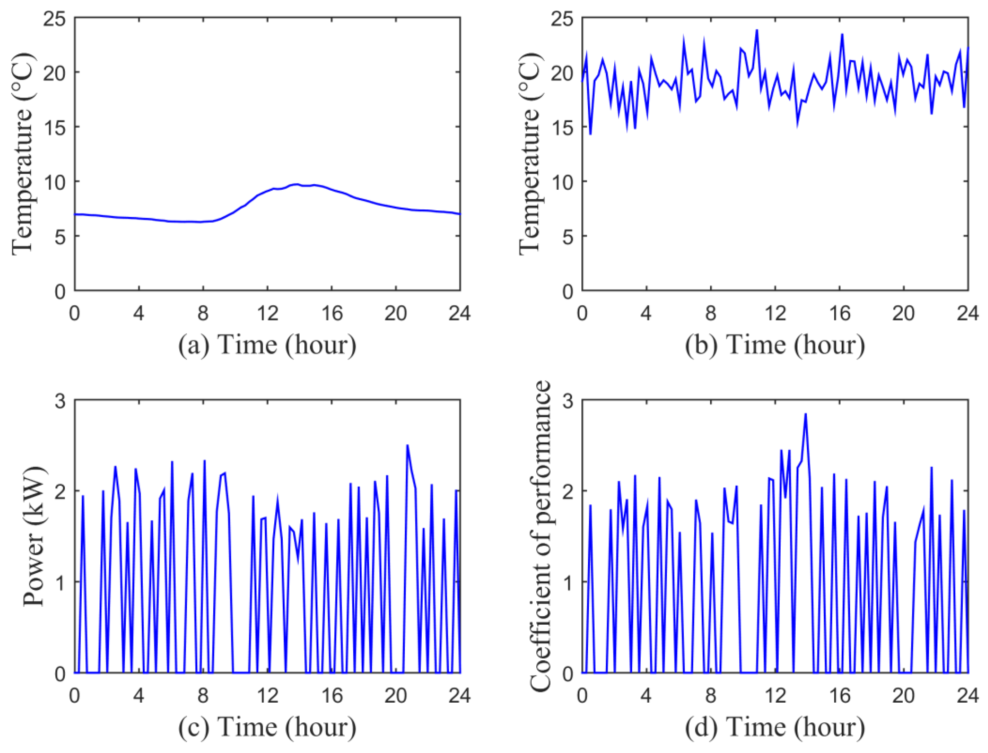
Figure 3.
In DNO14, (a) the thermal resistivity of modelled buildings using a uniform probabilistic distribution, while considering a normal probabilistic distribution to represent the following characteristics: (b) the coefficient of performance of the DHPs, (c) the climate-controlled temperatures of the buildings, and (d) the electricity loads of the DHPs.
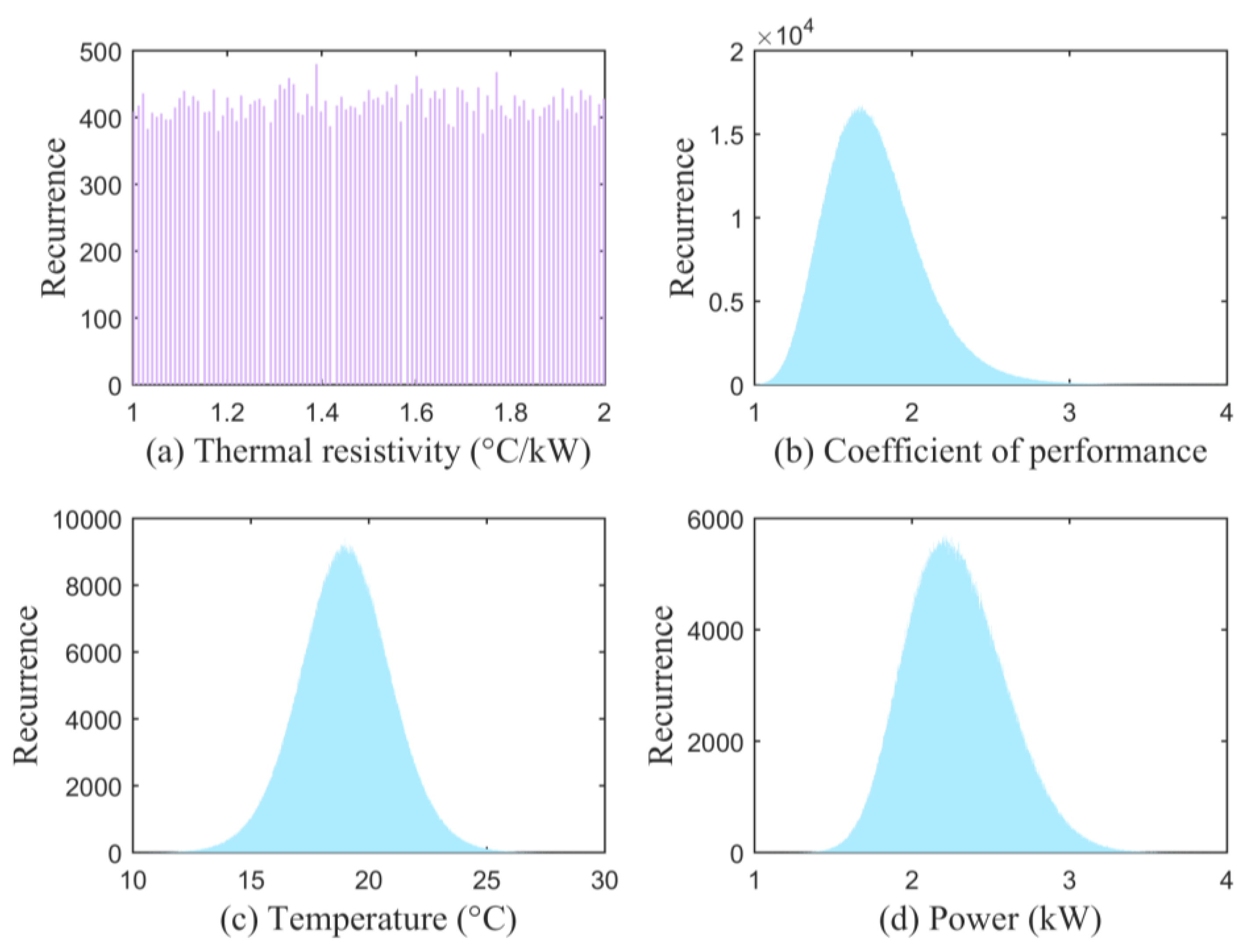
Figure 4.
A predicted overall demand of the DHPs for each DNO area by 2035.
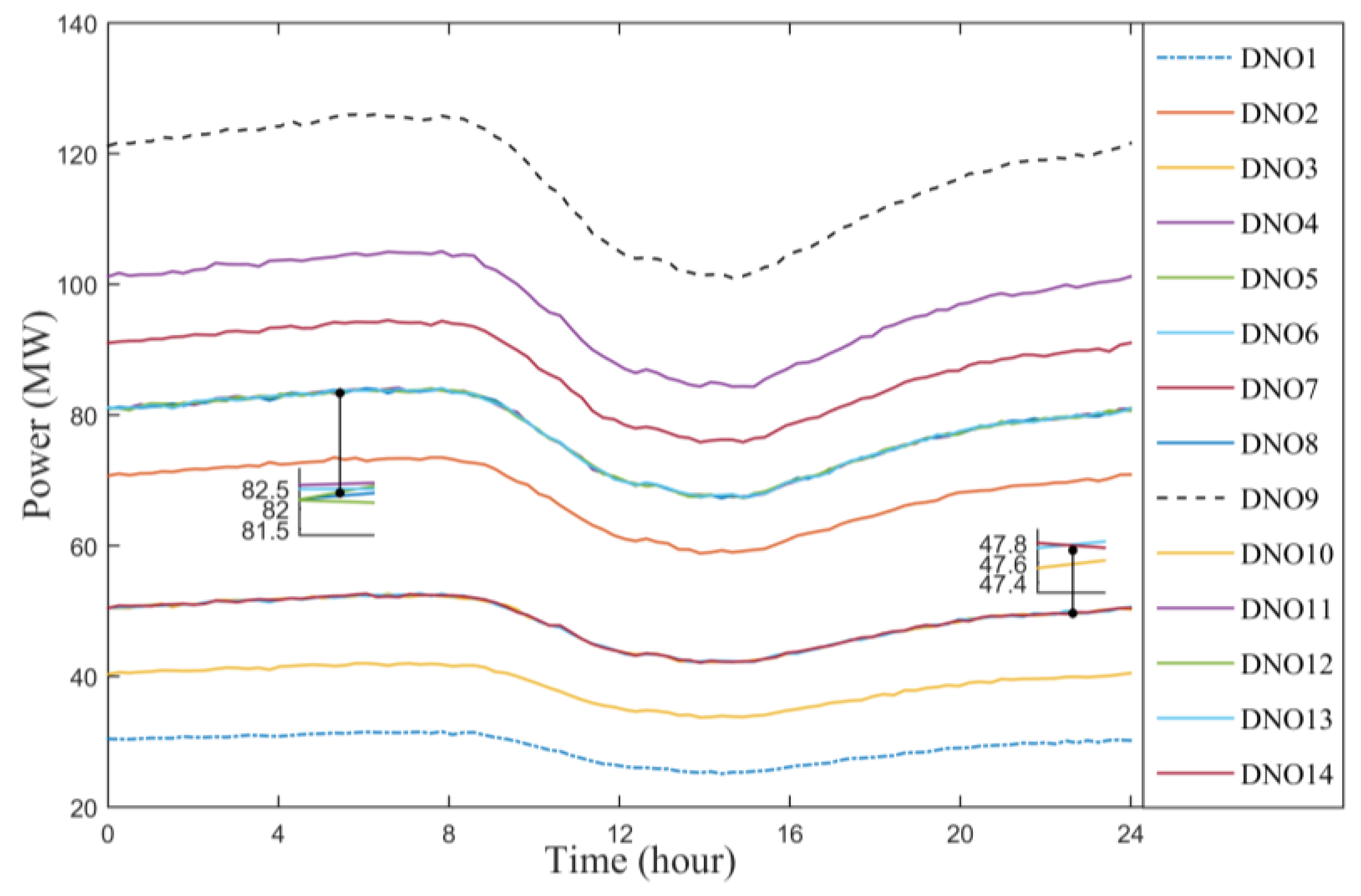
Figure 5.
Available demand reduction using the DHPs for each DNO area by 2035, considering the inside temperatures of buildings between 18–21°C.
Figure 5.
Available demand reduction using the DHPs for each DNO area by 2035, considering the inside temperatures of buildings between 18–21°C.
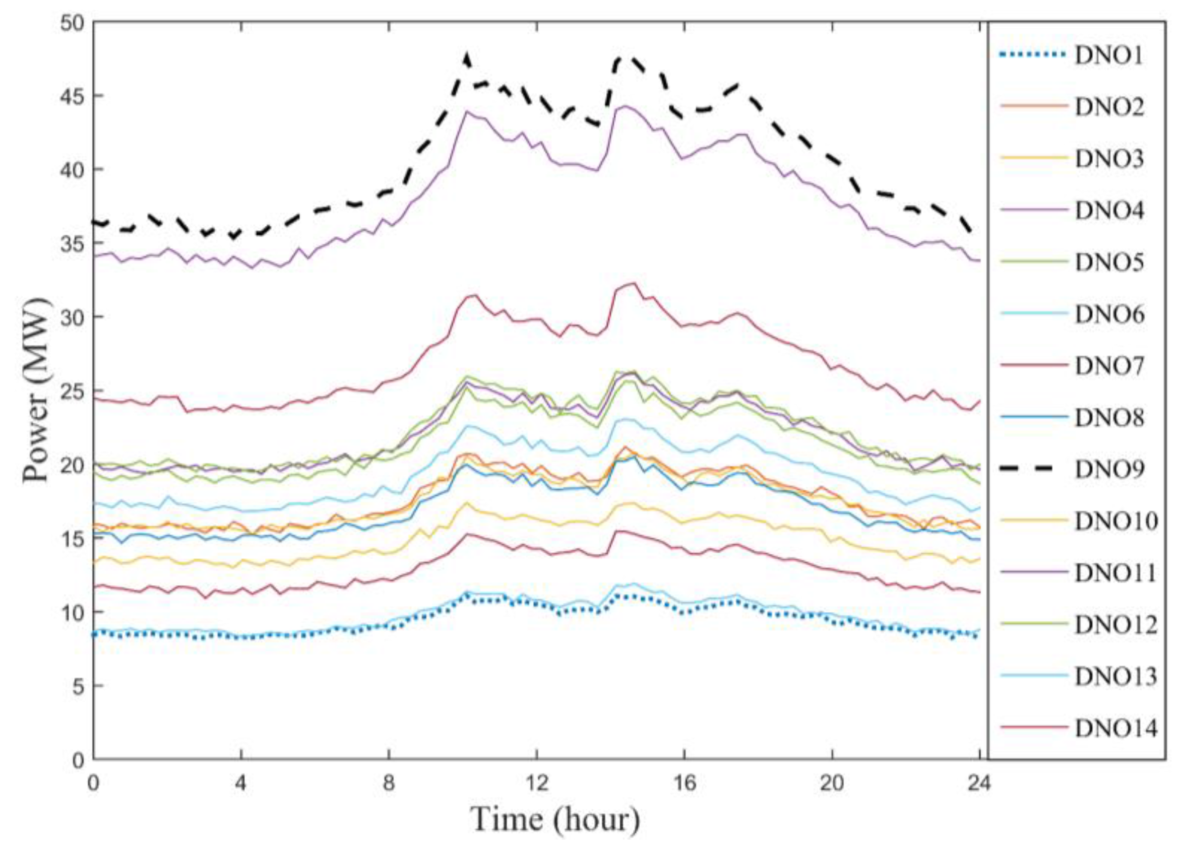
Figure 6.
System frequency (i.e., a 1.32 GW generation loss) without and with the dynamic controller, considering 1.05 GW power reserve of frequency-controlled DHPs in all DNO regions.
Figure 6.
System frequency (i.e., a 1.32 GW generation loss) without and with the dynamic controller, considering 1.05 GW power reserve of frequency-controlled DHPs in all DNO regions.
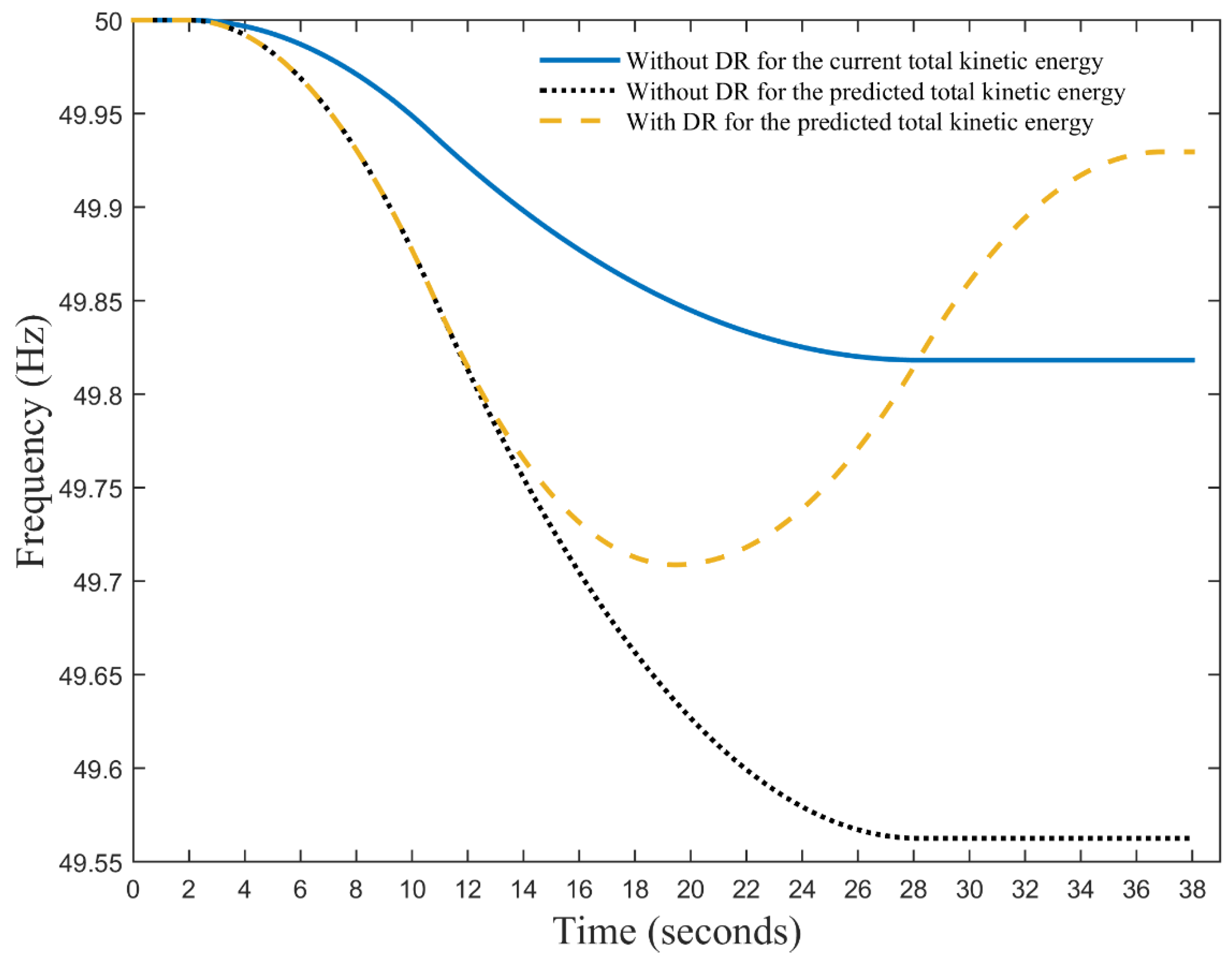
Figure 7.
System frequency (i.e., based on normal probabilistic deviations between supply and demand) without and with the static DR controller using demand reduction of frequency-controlled DHPs at DNO9 only.
Figure 7.
System frequency (i.e., based on normal probabilistic deviations between supply and demand) without and with the static DR controller using demand reduction of frequency-controlled DHPs at DNO9 only.
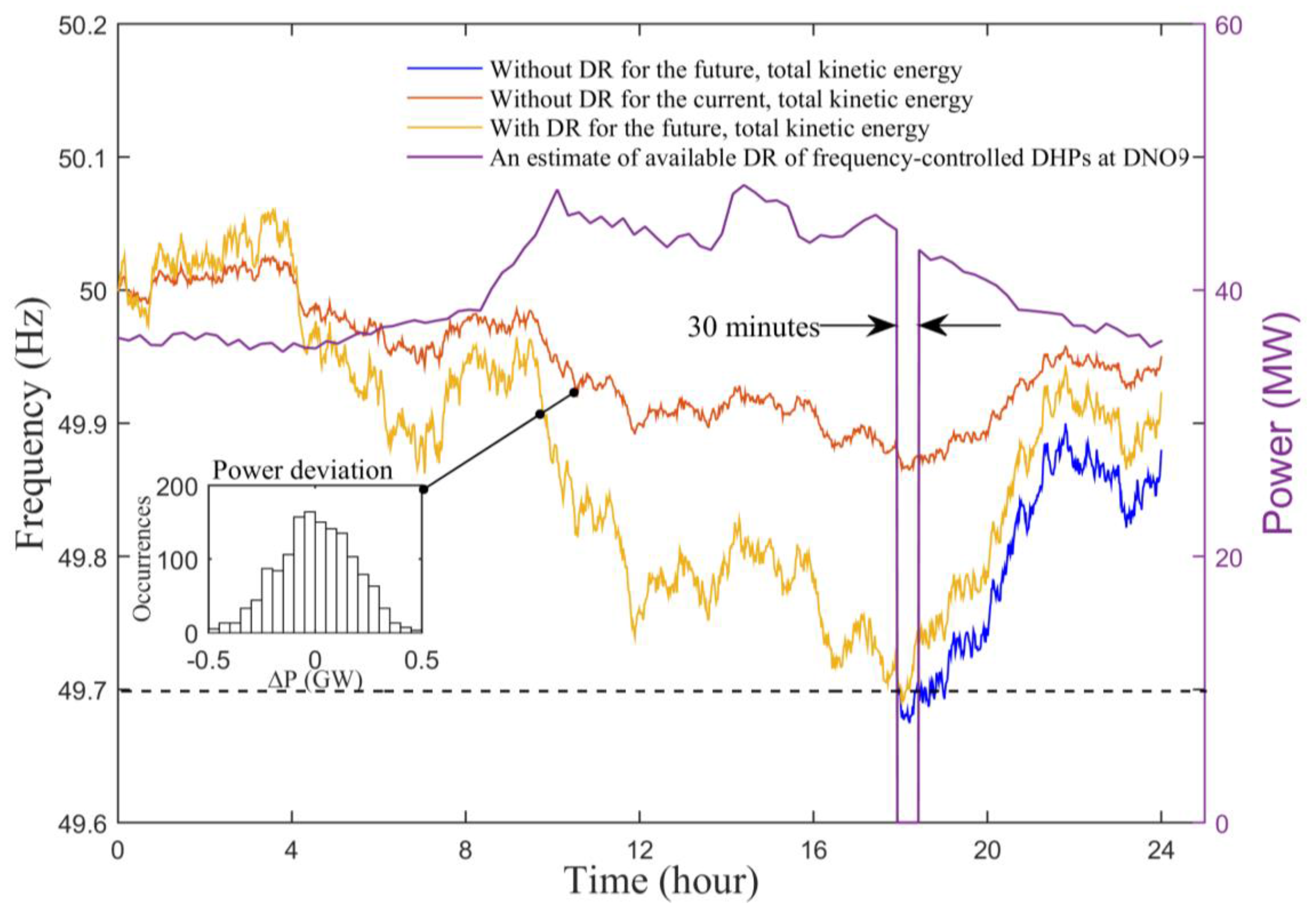
Figure 8.
Power share of demand reduction using the DHPs for each DNO area across the UK.
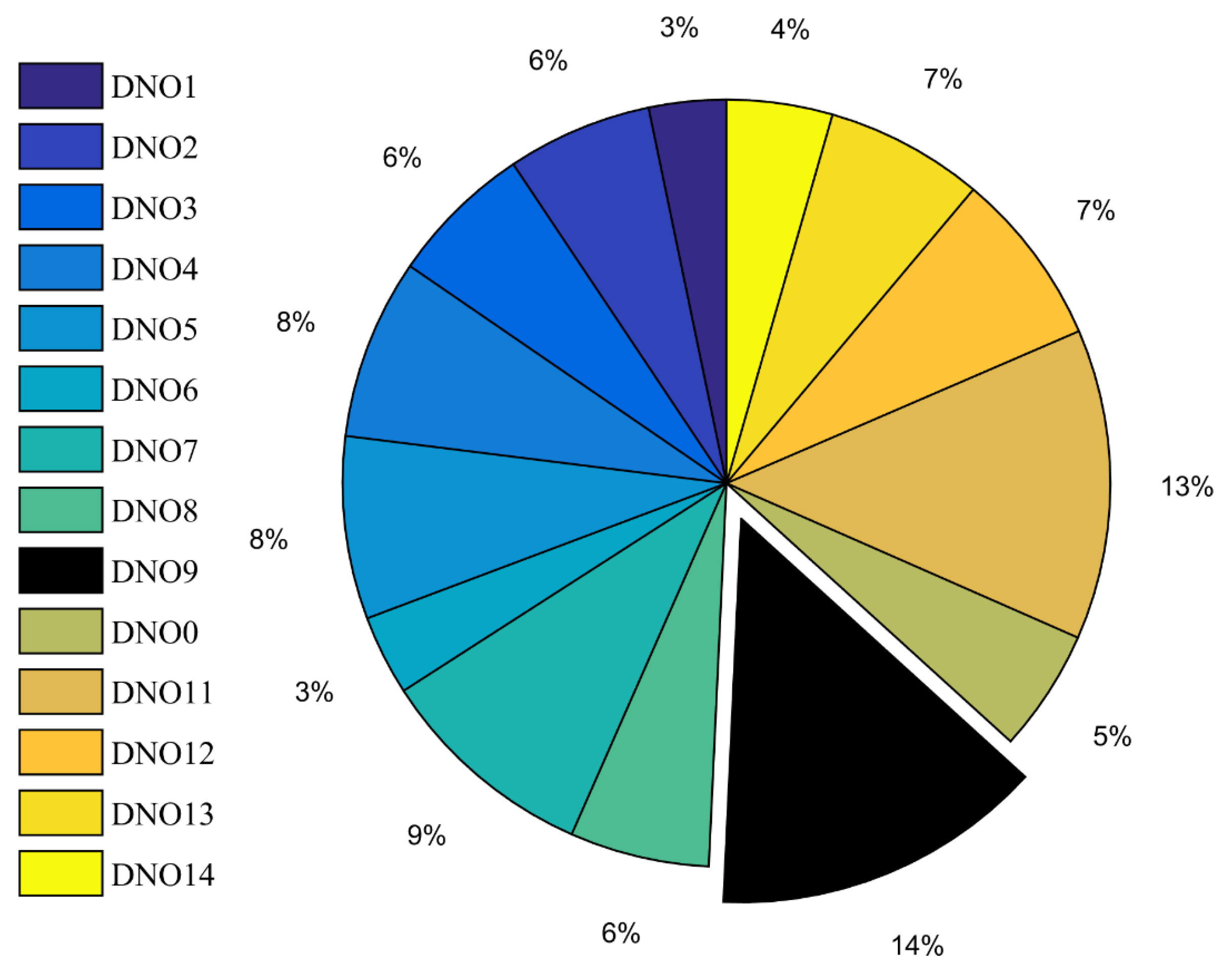
Figure 9.
An estimate of average demand reduction and average payment for the static/dynamic DR controller of DHPs for each DNO region in the UK based on the current electricity market.
Figure 9.
An estimate of average demand reduction and average payment for the static/dynamic DR controller of DHPs for each DNO region in the UK based on the current electricity market.

Table 1.
The considered parameters of domestic heat pumps (DHPs).
| Symbol | Quantity | Values | In Equations |
|---|---|---|---|
| air density | 1.2 kg/m3 | (5) and (7) | |
| specific heat of air | 1 kJ/kg°C | (5), (7) and (9) | |
| air flow rate | 0.5 m3/s | (5) and (7) | |
| supply temperature | 25 °C | (6) and (7) | |
| return temperature | 19 °C | (8) and (9) | |
| air mass flow | 1 kg/s | (9) |
Table 2.
The projected numbers of DHPs in the UK [9].
Table 2.
The projected numbers of DHPs in the UK [9].
| Year | The number of the DHPs | |
|---|---|---|
| High Scenario | Low Scenario | |
| 2020 | 386,200 | 183,252 |
| 2025 | 1,912,406 | 485,293 |
| 2030 | 3,306,832 | 713,964 |
| 2035 | 4,198,906 | 849,558 |
Table 3.
The predicted numbers of the DHPs for each distribution network operator (DNO) area in the UK by 2035 (i.e., using the low scenario of Table 2).
Table 3.
The predicted numbers of the DHPs for each distribution network operator (DNO) area in the UK by 2035 (i.e., using the low scenario of Table 2).
| The DNO Area | Predicted Numbers | The DNO Area | Predicted Numbers |
|---|---|---|---|
| DNO1 (North Scotland) | 25,487 | DNO8 (West Midlands) | 67,965 |
| DNO2 (South Scotland) | 59,469 | DNO9 (Eastern England) | 101,947 |
| DNO3 (North East England) | 42,478 | DNO10 (South Wales) | 33,982 |
| DNO4 (North West) | 67,965 | DNO11 (Southern England) | 84,956 |
| DNO5 (Yorkshire) | 67,965 | DNO12 (London) | 67,965 |
| DNO6 (Merseyside and N Wales) | 42,478 | DNO13 (South East England) | 67,965 |
| DNO7 (East Midlands) | 76,460 | DNO14 (South West England) | 42,478 |
Table 4.
An executive summary of the values of DR services in 2015/16 in the UK, as compared to their values in 2035 using the proposed DR controller.
Table 4.
An executive summary of the values of DR services in 2015/16 in the UK, as compared to their values in 2035 using the proposed DR controller.
| Year | Type of DR Services | Power Reserve | Payment |
|---|---|---|---|
| 2015/16 | Static and dynamic | 374 MW | £9.8m |
| 2035 | Static and dynamic | 663 MW | £17m |
© 2017 by the author. Licensee MDPI, Basel, Switzerland. This article is an open access article distributed under the terms and conditions of the Creative Commons Attribution (CC BY) license (http://creativecommons.org/licenses/by/4.0/).
Share and Cite
MDPI and ACS Style
Al Essa, M.J.M. Demand Response Design of Domestic Heat Pumps. Designs 2018, 2, 1. https://doi.org/10.3390/designs2010001
AMA Style
Al Essa MJM. Demand Response Design of Domestic Heat Pumps. Designs. 2018; 2(1):1. https://doi.org/10.3390/designs2010001
Chicago/Turabian StyleAl Essa, Mohammed Jasim M. 2018. "Demand Response Design of Domestic Heat Pumps" Designs 2, no. 1: 1. https://doi.org/10.3390/designs2010001