Adaptive Sliding Mode Control for High-Frequency Sampled-Data Systems with Actuator Faults


Harbin Institute of Technology, Harbin 150001, China
*
Author to whom correspondence should be addressed.
Designs 2018, 2(1), 3; https://doi.org/10.3390/designs2010003
Submission received: 14 December 2017
/
Revised: 11 January 2018
/
Accepted: 11 January 2018
/
Published: 17 January 2018
(This article belongs to the Special Issue Optimization, Health Monitoring and Control Methods for Modern Complex Systems)
Abstract
:This paper investigates the sliding mode control for high-frequency sampled-data systems with actuator faults. Besides matched nonlinearity, this paper also considers unmeasurable states and unknown actuator degradation ratio as important factors of the overall system. The estimates of system state vector are obtained by an adaptive sliding mode observer method firstly. Then, a novel integral-type sliding surface, corresponding to the unified closed-loop delta operator system, is provided based on aforementioned estimation values, and the fault closed-loop system is proven to be stable by the proposed sliding mode control law. Finally, the fault-tolerant control theory is verified to be valid via a practical simulation example.
1. Introduction
In practical engineering, unexpected faults of components including sensors and actuator and/or the system’s structure always occur inevitably in practice due to components burn-in, damage, physical constraint, etc. The impact of a fault or failure can lead to performance deterioration or instability of the systems, and could even cause unexpected catastrophic accidents. For example, an actuator of the vehicle system is stuck and failed to deflect the certain control state, which may result in a serious problem. Hence, developing effective fault-tolerance design techniques to accommodate sensor/actuator failures, and ensure high degree safe operation performances of the overall control systems has been an essential and significant issue in recent years [1,2,3], and some interesting results have been achieved [4,5,6,7]. In particular, adaptive control and sliding mode control methods have been applied to different systems to cope with sensor/actuator faults and unknown external disturbances (for instance, [8,9,10,11,12], and the references therein).
A great deal of attention has been paid to networked control systems (NCSs) in recent years [13,14,15,16,17], because they are able to be combined with different kinds of practical systems widely [18,19,20]. It should be noticed that, in modern industrial systems, the high frequency sampling situation always exists. Conventional discretization means derived from the model built for traditional systems failed to get the original system dynamic if the sampling time becomes more and more close to zero. However, the appearance of delta operator systems has worked out this restriction and the feature of high frequency sampling systems is able to be described accurately, the control result of using the delta operator approach is much better than applying shift operator method. For this reason, the delta operator systems have attracted abundant concern and many relevant theories such as control, adaptive control and sliding mode control methods have been applied on this issue.
The coexistence of sudden system structure change, high frequency data sampling [21], unknown model nonlinearity [22,23] and actuator faults in practical system makes it important to deal with the fault-tolerant control problems of the systems mentioned above, which motivates our work. In this paper, we simultaneously consider model nonlinearity and obtain the expected adaptive fault-tolerant control method for the delta operator system. First, the estimates of the state vector are derived from the proposed adaptive sliding mode observer and a special switching term is introduced to dispose the actuator faults. In addition, stability of the fault closed-loop system is guaranteed by the novel integral-type sliding mode controller we designed and the simulation result is presented in the end to prove the effectiveness of the method.
The structure of this paper is as follows. In Section 2, the existing problem is presented in detail. Section 3 and Section 4 introduce the stability criterion and develop the adaptive controller, respectively. The system trajectory is analyzed in Section 5 to illustrate its reachability and property. In Section 6, a practical problem is provided and the validity of the proposed method is proven by simulation results. Finally, the paper is concluded in Section 7.
2. Problem Statement
The delta operator owns the following form:
where T is the sampling period. In this paper, description of the following uncertain linear delta operator system is
where means the immeasurable system state, the signal from the hth faulted actuator in the lth faulty mode is presented by , , , the total number of faulty modes is L. is the measurable output, stands for the unknown sensor output. , and are system matrices with appropriate dimensions. means the unknown actuator efficiency factor which consist the diagonal matrix , definition of the unknown constant is
Define ; if and , it means that the hth actuator is outage in the lth fault mode, and stand for the fault-stuck problem on the hth actuator in the lth fault mode, means that effectiveness of the hth actuator is damaged in the lth fault mode, is the no fault state symbol of the hth actuator in the lth fault mode. is the unknown time-varying bounded fault-stuck in the hth actuator. For simplicity, in the following, the model is exploited by:
where .
The following assumptions are made in this paper.
- (A1)
- , where , are known constants.
- (A2)
- The actuator fault redundancy condition is that .
- (A3)
- The unknown time-varying bounded fault-deviation vector satisfies:where and stand for the unknown upper and lower bounds of , respectively, and we denote
Lemma 1.
[24] Considering known matrices and , assume that U has full column rank and . Then, holds for a scalar α if and only if where is any matrix whose columns are able to build the null space basis of .
The design of observer for the system in Equation (2) is as follows:
where means the estimation of , L is the observer gain to be designed, and stands for the discontinuous term. is the estimation of the actuator efficiency factor. and are estimations of and , ,
means the hth column of B, is the Lyapunov matrix to be designed. The definition of sliding surface is as follows:
Define the error ; the error dynamic can be obtained as follows:
Let , then rewrite the sliding surface in Equation (9) as:
Using the following coordinate transformation
with and , is any basis of the null space of , . Then, it can be obtained that
In this situation, we can obtain the reduced-order sliding mode dynamics for the sliding surface
Then, we analyze the stochastic stability of the sliding mode Equation (14).
3. Stability Analysis of the Sliding Motion Equation
In this section, the reduced-order sliding mode dynamics will be analyzed to guarantee the stochastic stability of the overall system.
Theorem 1.
The reduced-order sliding mode dynamics in Equation (14) is stochastic stable in delta domain, if there exists a matrix with appropriate dimension, and scalars such that the following LMI holds
with
Proof.
In delta domain, define a Lyapunov functional as follows:
Based on Lemma 1, and taking the delta operator manipulations of along the trajectory of delta operator system, we can obtain:
Thinking about the certain zero term
Then, it can be obtained that
holds if
with
which is equivalent to
It is not difficult to derive from Lemma 2 that is solvable for and if and only if the following holds
the formulation is equivalent to
Pre- and post-multiplying (26) by and its transpose, we have
where , , then Equation (28) can be rewritten as:
4. Stability Analysis of the Error Dynamic
This section will focus on designing the discontinuous term to guarantee the stochastic stability of the error system in Equation (10). can be designed as
with the sliding surface in Equation (9). Moreover, the adaption laws are given as follows:
Theorem 2.
With the sliding mode controller , the error system in Equation (10) is stochastic stable if the following matrix constraint is satisfied:
Proof.
Define Lyapunov function and the error variable
Taking the stochastic delta operator manipulations of along the trajectory of system, we obtain:
Recalling , Equation (39) becomes
In Equation (40) the term can be amplified as:
Then, the expression of will become:
Substituting sliding mode controller into Equation (42), it can be obtained that:
Hence, we can see that
For the Lyapunov function , it can be derived that the can described as:
then, we can rewrite the expression of as:
It should be noticed that, if we select a small enough sampling interval T, the terms containing T are able to be suppressed, and the expression becomes:
Let , then, it can be obtained that
Note that
define
The estimation of , which is and can be adjusted according to the adaptive laws:
In addition, and are updated by the adaptive laws:
then, the formulation of will be rewritten as:
Choose appropriate constants and satisfying . Then, the stability condition will be obtained:
It is obvious that is correct if the matrix inequality in Equation (38) holds, which completes the proof. ☐
5. Section Stabilization of the Overall Closed-Loop Systems
The overall closed-loop system is described as follows:
then, the sliding surface will be written as:
where F is designed such that is non-singular, and is designed to meet that is Hurwitz. It can be seen that:
For , it can be obtained that
For , it is calculated that
Thus, it is easy to derive that:
According to the definition of , it can be derived that:
If , it can be obtained that:
Therefore, the equivalent control law can be written as:
Based on the observer equation, the present objective is to design to ensure that the closed-loop system is able to be driven onto the sliding surface with probability 1 in finite time.
The can be defined as
with
Theorem 3.
Supposing Inequalities (15) and (38) have solutions, the sliding surface is given by Equation (53). Then, the trajectory of delta operator system in Equation (52) can be driven onto the sliding surface in finite time with the following control law in Equation (62), and evolve in a neighborhood around the sliding surface, converging to a residual set at the origin in the end.
Proof.
Considering , define a Lyapunov function ,
It should be noticed that the following fact holds:
In addition, considering and the control law, there will exist
The term in the above inequality contains the parameter uncertainties and a properly selected can suppress the uncertainty. If the parameter uncertainties are large, the sampling interval q should be selected small to guarantee that the term becomes small enough. Appropriately selecting parameter , it can be obtained that
where and are proper positive scalars. We can derive that
The proof is completed. ☐
6. Numerical Example
We provide an example to prove the validity of the results mentioned above in this section. The proposed method will be applied to design a robust sliding mode controller for the simplified truck-trailer system, which was proposed as in [25], and the system associated with delta operator is described as
with
Define the sampling period as and the actuator efficiency value as . The original state of system can be chosen as , .
After solving matrix constraint in Equation (15), the following solution can be obtained that:
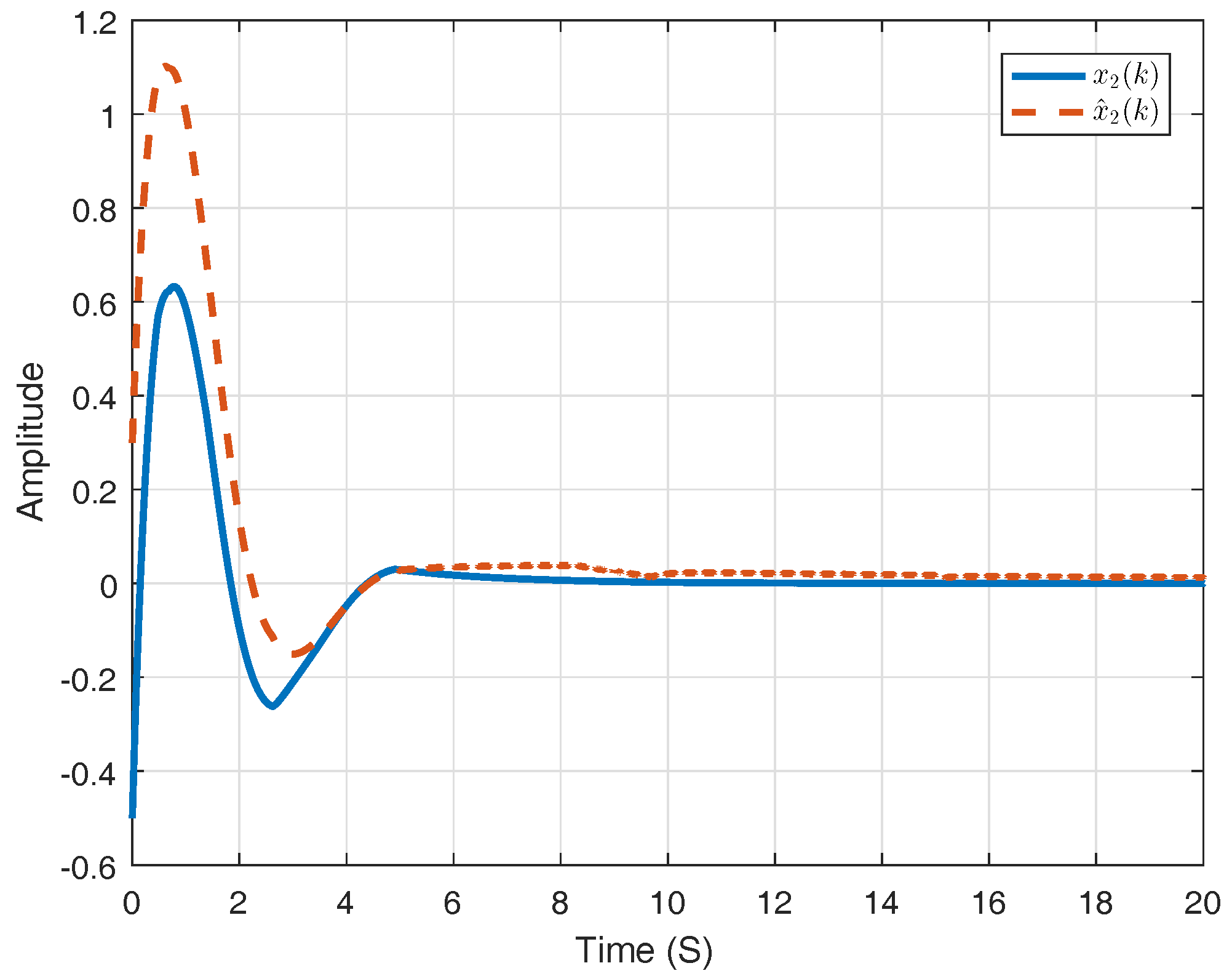
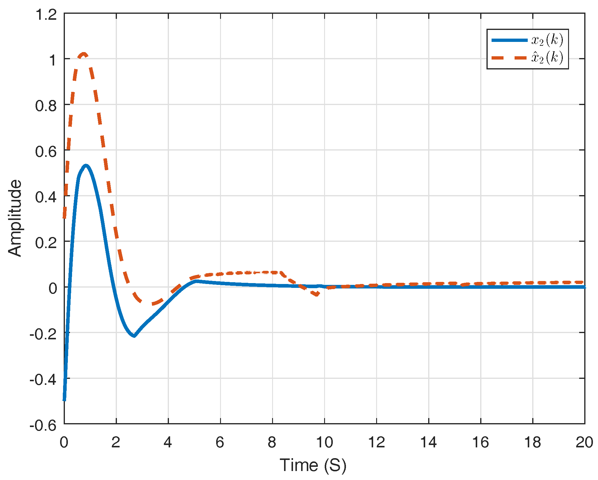
Figure 1 shows the sliding surface applied in the -domain, which can be denoted by . Considering state variable , Figure 2 and Figure 3 compare the corresponding state trajectories of system and its observer. It is easy to conclude that the system is stochastically stable. Figure 4 and Figure 5 compare the current results with the consequences gotten by the methods in previous work.
7. Conclusions
In this paper, we have investigated delta operator method to research the adaptive sliding mode control for high-frequency sampled-data systems with actuator faults. A novel observer-based sliding mode control method is proposed to deal with the problem. In future work, we will pay attention to the situation in which is influenced by network-induced communication delay and data packet losses are taken into account, simultaneously. In the future, we will focus on the combination of delta operator with semi-Markov systems, switched positive system, etc. and consider the influence of dead-zone or saturation to the overall system.
Author Contributions
Dongyang Zhao, Yu Liu and Ming Liu conceived and designed the experiments; Dongyang Zhao performed the experiments; Dongyang Zhao and Ming Liu analyzed the data; Jinyong Yu contributed reagents/materials/analysis tools; Dongyang Zhao wrote the paper.
Conflicts of Interest
The authors declare no conflict of interest.
References
- Liu, H.H.T.; Shi, P.; Jiang, B. Fault detection, diagnosis, and fault tolerant control with flight applications. J. Frankl. Inst. 2013, 350, 2371–2372. [Google Scholar] [CrossRef]
- Jiang, B.; Wang, J.L. Actuator fault diagnosis for a class of bilinear systems with uncertainty. J. Frankl. Inst. 2002, 339, 361–374. [Google Scholar] [CrossRef]
- Li, L.; Chadli, M.; Ding, S.X.; Qiu, J.; Yang, Y. Diagnostic Observer Design for TS Fuzzy Systems: Application to Real-Time Weighted Fault Detection Approach. IEEE Trans. Fuzzy Syst. 2017. [Google Scholar] [CrossRef]
- Hao, L.Y.; Yang, G.H. Robust fault tolerant control based on sliding mode method for uncertain linear systems with quantization. ISA Trans. 2013, 52, 600–610. [Google Scholar] [CrossRef] [PubMed]
- Rios, H.; Kamal, S.; Fridman, L.M.; Zolghadri, A. Fault tolerant control allocation via continuous integral sliding-modes: A HOSM-Observer approach. Automatica 2015, 51, 318–325. [Google Scholar] [CrossRef]
- Youssef, T.; Chadli, M.; Karimi, H.R.; Wagn, R. Actuator and sensor faults estimation based on proportional integral observer for TS fuzzy model. J. Frankl. Inst. 2017, 354, 2524–2542. [Google Scholar] [CrossRef]
- Saifia, D.; Chadli, M.; Labiod, S.; Guerra, T.M. Robust H∞ static output feedback stabilization of TS fuzzy systems subject to actuator saturation. Int. J. Control Autom. Syst. 2012, 10, 613–622. [Google Scholar] [CrossRef]
- Niu, Y.; Ho, D.W.C. Control strategy with adaptive quantizer’s parameters under digital communication channels. Automatica 2014, 50, 2665–2671. [Google Scholar] [CrossRef]
- Li, Y.; Tong, S.; Liu, Y.; Li, T. Adaptive Fuzzy Robust Output Feedback Control of Nonlinear Systems with Unknown Dead Zones Based on a Small-Gain Approach. IEEE Trans. Fuzzy Syst. 2014, 22, 164–176. [Google Scholar] [CrossRef]
- Liu, D.; Wei, Q. Policy iteration adaptive dynamic programming algorithm for discrete-time nonlinear systems. IEEE Trans. Neural Netw. Learn. Syst. 2014, 25, 621. [Google Scholar] [PubMed]
- Su, J.; Chen, W.H. Model-based fault diagnosis system verification using reachability analysis. IEEE Trans. Syst. Man Cybern. Syst. 2017. [Google Scholar] [CrossRef]
- Yu, S.; Yu, X.; Shirinzadeh, B.; Man, Z. Continuous finite-time control for robotic manipulators with terminal sliding mode. Automatica 2005, 41, 1957–1964. [Google Scholar] [CrossRef]
- Shah, D.H.; Mehta, A.J. Multirate output feedback based discrete-time sliding mode control for fractional delay compensation in NCSs. In Proceedings of the IEEE International Conference on Industrial Technology, Toronto, ON, Canada, 22–25 March 2017. [Google Scholar]
- Mathiyalagan, K.; Ju, H.P.; Sakthivel, R. New results on passivity-based H∞ math Container Loading Mathjax, control for networked cascade control systems with application to power plant boiler-turbine system. Nonlinear Anal. Hybrid Syst. 2015, 17, 56–69. [Google Scholar] [CrossRef]
- Du, D.J.; Qi, B.; Wang, Z.X.; Fei, M.R.; Peng, C. Distributed event-triggered hybrid wired-wireless networked control with H2/H∞, filtering. Memet. Comput. 2017, 9, 55–86. [Google Scholar] [CrossRef]
- Wang, H.; Shi, P.; Zhang, J. Event-triggered fuzzy filtering for a class of nonlinear networked control systems. Signal Process. 2015, 113, 159–168. [Google Scholar] [CrossRef]
- Wei, Y.; Park, J.H.; Karimi, H.R.; Tian, Y.C.; Jung, H. Improved Stability and Stabilization Results for Stochastic Synchronization of Continuous-Time Semi-Markovian Jump Neural Networks With Time-Varying Delay. IEEE Trans. Neural Netw. Learn. Syst. 2017, 1–14. [Google Scholar] [CrossRef] [PubMed]
- Niu, Y.; Jia, T.; Wang, X.; Yang, F. Output-feedback control design for NCSs subject to quantization and dropout. Inf. Sci. 2009, 179, 3804–3813. [Google Scholar] [CrossRef]
- Qu, F.L.; Guan, Z.H.; He, D.X.; Chi, M. Event-triggered control for networked control systems with quantization and packet losses. J. Frankl. Inst. 2015, 352, 974–986. [Google Scholar] [CrossRef]
- Tang, X.; Ding, B. Model predictive control of linear systems over networks with data quantizations and packet losses. Automatica 2013, 49, 1333–1339. [Google Scholar] [CrossRef]
- Nguyen, T.; Su W, C.; Gajic, Z. Output feedback sliding mode control for sampled-data systems. IEEE Trans. Autom. Control 2010, 55, 1684–1689. [Google Scholar]
- Bououden, S.; Chadli, M.; Karimi, H.R. Fuzzy sliding mode controller design using Takagi-Sugeno modelled nonlinear systems. Math. Probl. Eng. 2013, 2013, 734094. [Google Scholar] [CrossRef]
- Su, J.; Yang, J.; Li, S. Continuous finite-time anti-disturbance control for a class of uncertain nonlinear systems. Trans. Inst. Meas. Control 2014, 36, 300–311. [Google Scholar] [CrossRef]
- Iwasaki, T.; Skelton, R.E. All Controllers for the General, H∞, Control Problem: LMI Existence Conditions and State Space Formulas; Pergamon Press, Inc.: Oxford, UK, 1994. [Google Scholar]
- Qiu, J.; Xia, Y.; Yang, H.; Zhang, J. Robust stabilisation for a class of discrete-time systems with time-varying delays via delta operators. IET Control Theory Appl. 2008, 2, 87–93. [Google Scholar] [CrossRef]
Figure 1.
The figure of .
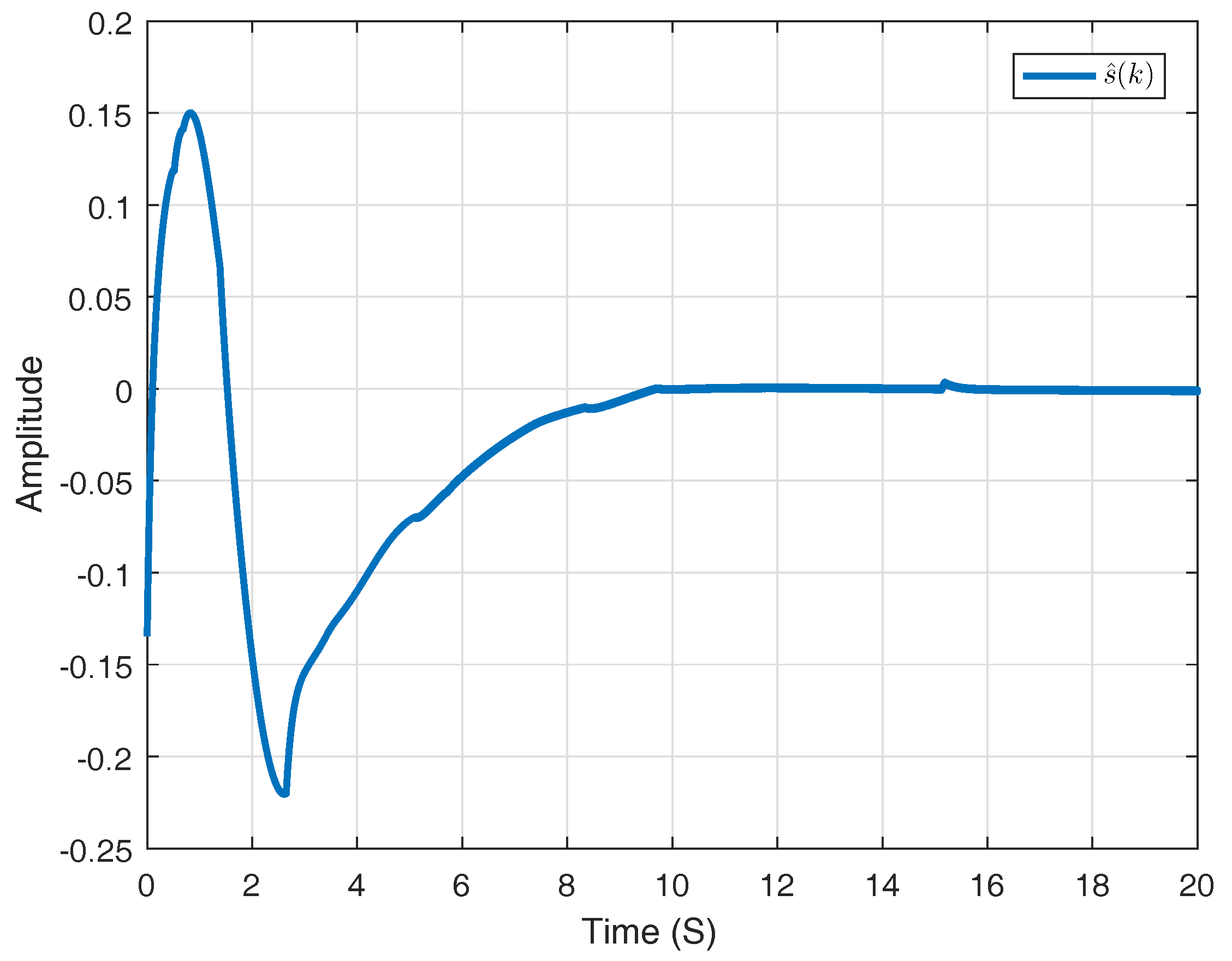
Figure 2.
State component and its estimation.
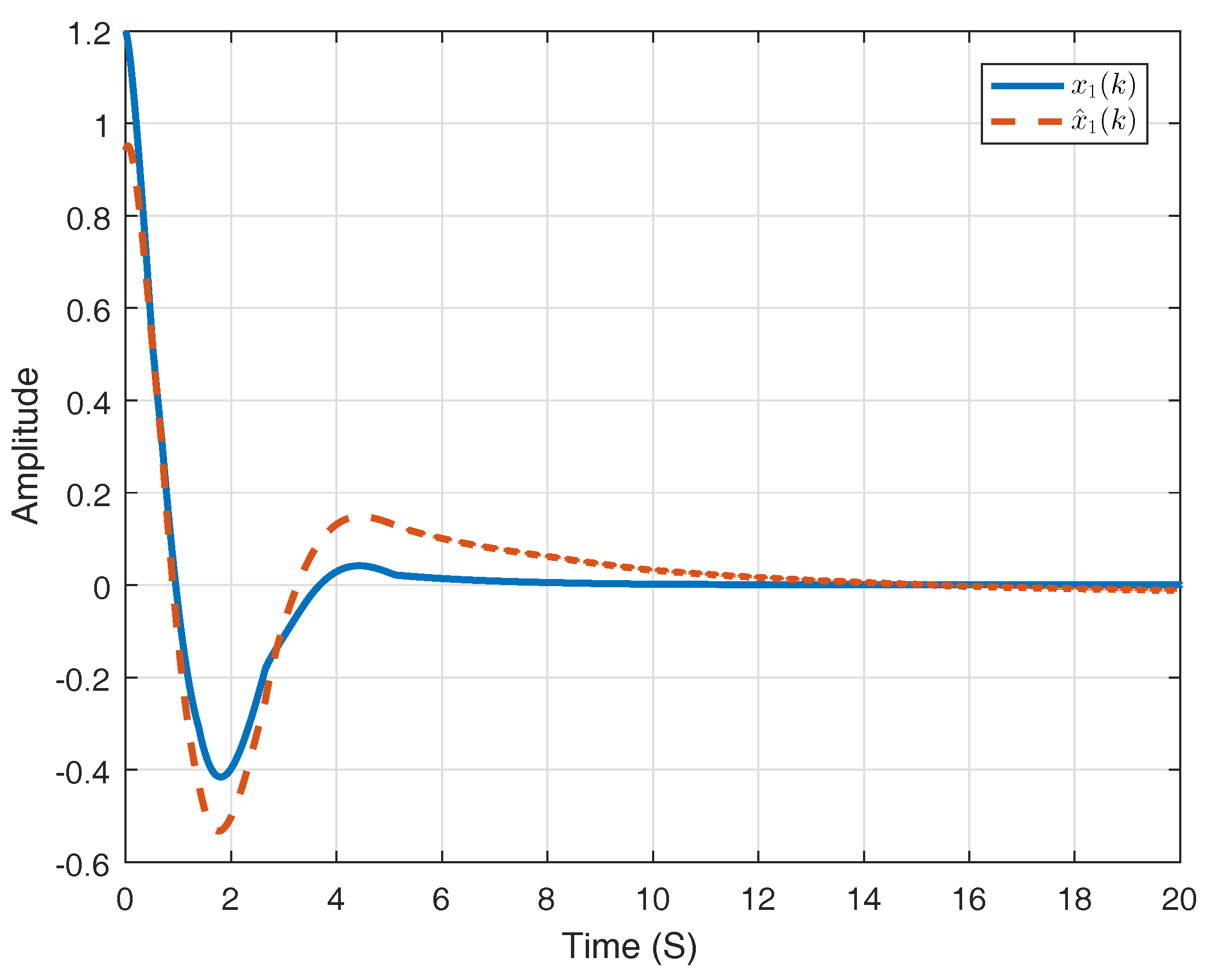
Figure 3.
State component and its estimation.

Figure 4.
and its estimation in previous work.
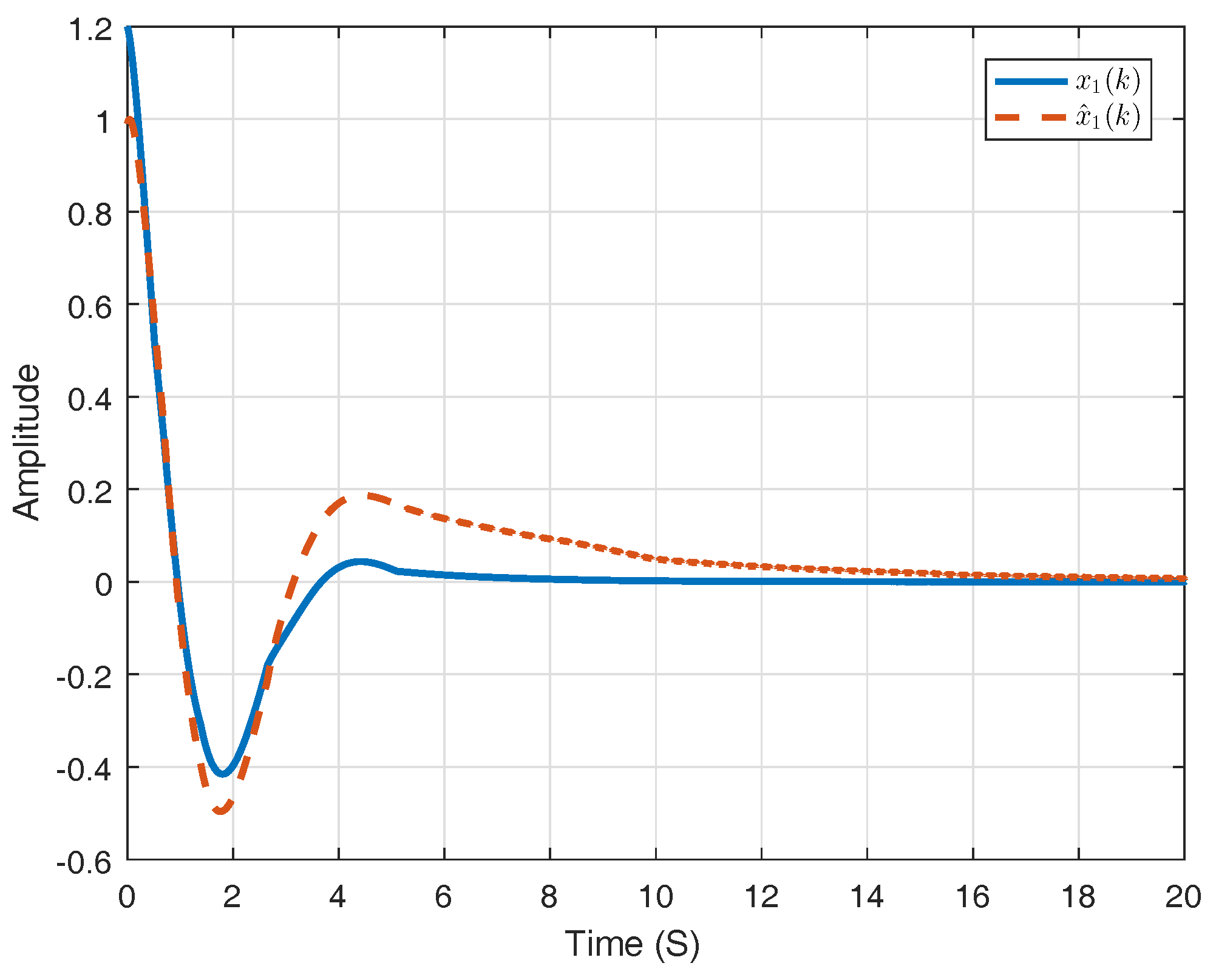
Figure 5.
and its estimation in previous work.
© 2018 by the authors. Licensee MDPI, Basel, Switzerland. This article is an open access article distributed under the terms and conditions of the Creative Commons Attribution (CC BY) license (http://creativecommons.org/licenses/by/4.0/).
Share and Cite
MDPI and ACS Style
Zhao, D.; Liu, Y.; Liu, M.; Yu, J. Adaptive Sliding Mode Control for High-Frequency Sampled-Data Systems with Actuator Faults. Designs 2018, 2, 3. https://doi.org/10.3390/designs2010003
AMA Style
Zhao D, Liu Y, Liu M, Yu J. Adaptive Sliding Mode Control for High-Frequency Sampled-Data Systems with Actuator Faults. Designs. 2018; 2(1):3. https://doi.org/10.3390/designs2010003
Chicago/Turabian StyleZhao, Dongyang, Yu Liu, Ming Liu, and Jinyong Yu. 2018. "Adaptive Sliding Mode Control for High-Frequency Sampled-Data Systems with Actuator Faults" Designs 2, no. 1: 3. https://doi.org/10.3390/designs2010003