
Machine Learning and Optimality in Multi Storey Reinforced Concrete Frames


Department of Production Engineering and Management, Technical University of Crete, 731 00 Chania, Greece
*
Author to whom correspondence should be addressed.
Infrastructures 2017, 2(2), 6; https://doi.org/10.3390/infrastructures2020006
Submission received: 25 January 2017
/
Revised: 7 April 2017
/
Accepted: 22 April 2017
/
Published: 3 May 2017
(This article belongs to the Special Issue Concrete Structures: Present and Future Trends)
Abstract
:The present study investigates the potential of the implementation of machine learning techniques in optimized multi storey reinforced concrete frames. The variables that are taken into account in the objective function of the optimization problem are the following: the frame type (frame bay length optimality) and dimensioning of the cross sections. The objective function has the goal of attaining a minimum cost design based on market data, after a structural analysis of the frames. A number of optimized examples with widely encountered cases of total lengths of frames and with various loadings are presented. Modeling is based on Eurocode 2. Optimization takes place with the use of evolutionary algorithms. The optimized results are subjected to predictive modeling based on neural networks. The objective of the study is to create predictive models with the aim of minimizing the usage of scarce resources.
1. Introduction
1.1. Initial Considerations
In the structural design of frames used in buildings, a structural analysis first takes place for the determination of the axial, shear forces, and moments of every member (beams and columns) [1]. Following this, the beams and columns are dimensioned to resist the axial, shear forces, and moments that arise. The total cost of a frame is therefore a sum that is dependent on its form and on the sizes of its beams and columns [2].
In reinforced concrete buildings, a very common formula used to evaluate the cost of each component is the following:
where: Cconcrete, Csteel reinforcement, and Cformwork, respectively, are the costs of concrete, steel reinforcement, and formwork in RC elements [2].
From an overview of the relevant literature, the following conclusions can be drawn:
Well-known examples regarding the optimization of RC structures include the works of: Krishnamurthy and Munro [6] (where linear programming was employed for the optimization of RC frames), Lee and Ahn [7] and Camp, Pezeshk & Hansson [8] (where genetic algorithms and discrete optimization were used for the optimization of RC frames), and Guerra and Kiousis [9] (where Sequential Quadratic Programming was implemented for the same purposes). As far as the implementation of Artificial Neural Networks is concerned, Yousif et al. [10] have proposed ANN-based techniques for the purpose of forecasting the resistance of a structure, by using critical structural variables such as the material strength and loading conditions as predictors.
One of the main concerns of structural designers when using frames with multiple bays is to opt for economic solutions. Since such designs depend on the number of bays of the frames, the length of the bays, and the sizes of the beam and column cross sections, optimization techniques can be implemented to effectively deal with the computational difficulties which arise when assessing the large number of potential design solutions.
In light of this, the objective of the present study is to demonstrate a method to construct a predictive model based on machine learning to predict optimality in reinforced concrete frames with multiple storeys. The potential benefits of constructing a machine learning model deal with the minimization of the time required to predict optimality. The study focuses on presenting a method for the attainment of optimality from a cost standpoint, emphasizing the structural capacity of RC frames. With respect to the optimization of the frame structural costs, the present study faces this issue as a discrete optimization problem [11].
1.2. Programming Logic Followed for the Construction of the FEM Algorithm
A 2D finite element frame analysis framework has been followed for the construction of an algorithm in MATLAB [12,13]. A uniformly distributed load is assumed to be applied on the frame. This is a loading case that is commonly encountered in real life building structures. Initially, an estimation of the number of structural elements needed (beams and columns) was made according to empirical criteria (preliminary sizing) [14]. It was therefore considered that the number of elements would be five at a minimum and 19 at a maximum. As a result of this, eight different scenarios were included in the algorithm. Since the algorithm conducts the structural analysis through the finite element method, it is meaningful to mention several details about the procedure. The algorithm has been developed in MATLAB [12,13] in a way that makes it possible to solve a frame regardless of its total number of elements and by having observed the repeated patterns of the nodes -and accordingly the degrees of freedom- of every beam and column, the applied fixed end moments and shear forces to every start and end beam element node, the applied axial loads on the end or on the intermediate columns, and of the prescribed degrees of freedom. The reader should pay attention to the fact that the number of columns is always odd and the number of beams is always even, and the following relationship is always true [11]:
This consideration has critically influenced the programming logic. Furthermore, the number of elements has a constant relationship with the number of nodes (number of nodes = number of elements + 1) and the number of degrees of freedom (number of degrees of freedom = 3 × number of nodes).
Even though there are also other possible programming approaches, for reasons of predictability, the numbering logic of the degrees of freedom in the finite element algorithm that was constructed in MATLAB and the programming logic is as follows [12]:
where: the term elementDof stands for the degrees of freedom of each element; indice is the start or end index of a node; and numberNodes is a parameter equal to the total number of nodes of a frame, assisting in the arrangement of the global stiffness matrix and the identification of each degree of freedom.
elementDof = [indice indice + numberNodes indice + 2*numberNodes]
The first term of the above matrix stands for the axial displacements’ degrees of freedom, the second for the shear displacements’ degrees of freedom, and the last for the degrees of freedom that concern the elements’ moments [12,13].
The degrees of freedom are used in the construction of the global stiffness matrix, as well as in the start and end nodes of every frame element, regardless of the number of bays, following the node numbering logic shown in the figure below. This consideration has critically influenced the programming logic. The effect that this relationship has on the node numbering logic is demonstrated below (Figure 1).
It is evident that the repeated pattern of the numbering logic renders the nodes -and accordingly the degrees of freedom- of every beam and column quite easy to predict. Therefore, for a frame with three storeys, the beams have the indices that are displayed below:
where: the colon punctuation (:) represents the increment measured in an integer number of nodes, with a start point at the bottom left column node. The logic shown above is similar to the one used in the MATLAB algorithm that was constructed. The term numberofstoreys represents the number of storeys of the examined frame and the term lastnode represents the node that concerns the last node according to the numbering logic displayed in Figure 1.
Beam nodes first floor: [2:numberofstoreys + 1):(lastnode − (numberofstoreys − 1))]
Beam nodes second floor: [3:(numberofstoreys + 1):(lastnode − (numberofstoreys − 2))]
Beam nodes third floor: [4:(numberofstoreys + 1):(lastnode)]
Beam nodes second floor: [3:(numberofstoreys + 1):(lastnode − (numberofstoreys − 2))]
Beam nodes third floor: [4:(numberofstoreys + 1):(lastnode)]
Apart from this, since the lower end of all columns at the lowest storey is considered to be fixed, the repeatability of the prescribed degrees of freedom is shown in the following pseudocode [12], demonstrating the programming logic that has been followed:
where: the term prescribedDof represents the prescribed degrees of freedom that are the bottom end nodes of each column element at the lowest storey and the term numberofelements represents the number of elements that are dependent on the form of the frames.
prescribedDof1 = [1:(numberofstoreys + 1):(lastnode − (numberofstoreys))]
prescribedDof2 = [1:(numberofstoreys + 1):(lastnode − (numberofstoreys))] + numberofelements
prescribedDof3 = [1:(numberofstoreys + 1):(lastnode − (numberofstoreys))] + 2*numberofelements
prescribedDof = [prescribedDof1,prescribedDof2,prescribedDof3]
It is also meaningful to note that the connectivities among the elements were expressed in the algorithm as preset options, following the aforementioned numbering logic and corresponding to the number of bays of each frame type. After the solution of a frame, it becomes possible for the design moments, axial forces, and shear forces to be calculated and used for the dimensioning of the cross sections.
2. Optimization Procedure and Variables
The optimization procedure aimed to simulate as variables all of the parameters that a structural designer takes into consideration when opting for a frame. Specifically, these are: the number of bays of a frame, the cross sections of all the columns that constitute the frame, the cross sections of all the beams that constitute the frame, and the length of each separate beam. As is mentioned above, the selection of the range of the potential options for each variable is also based on empirical criteria [14]. After the completion of the finite element analysis that is conducted in MATLAB [12], the frame components are optimized by taking into account the following variables:
- Variable related to the form of the frames whose change influences the number of bays (eight possible choices leading to a total number of beam-column elements between five and 19).
- Variables related to the lengths of the beams. Each front beam length is considered to have a value between 3 and 7.5 m, with a step size of 0.5 m.
- Variables related to the cross sections of the beams of each storey that compose the structural frames. For all the frame scenarios, the following beam cross sections were considered: b = 350 mm h = 550 mm ρ = 1%, b = 350 mm h = 550 mm ρ = 2%, b = 350 mm h = 550 mm ρ = 3%, b = 350 mm h = 550 mm ρ = 4%, b = 350 mm h = 550 mm ρ = 5%, b = 350 mm h = 550 mm ρ = 6%, b = 350 mm h = 600 mm ρ = 1%, b = 350 mm h = 600 mm ρ = 2%, b = 350 mm h = 600 mm ρ = 3%, b = 350 mm h = 600 mm ρ = 4%, b = 350 mm h = 600 mm ρ = 5%, and b = 350 mm h = 600 mm ρ = 6% (where: b is the smaller dimension of the cross section, h is the larger dimension of the cross section, and ρ is the steel reinforcement ratio of the cross section).
- Variables related to the cross sections of the columns (each storey is examined separately) that compose the structural frames. For all the frame scenarios, the following column cross sections were considered: b = 350 mm h = 350 mm ρ = 1%, b = 350 mm h = 350 mm ρ = 2%, b = 350 mm h = 350 mm ρ = 3%, b = 350 mm h = 400 mm ρ = 1%, b = 350 mm h = 400 mm ρ = 2%, b = 350 mm h = 400 mm ρ = 3%, b = 400 mm h = 400 mm ρ = 1%, b = 400 mm h = 400 mm ρ = 2%, b = 400 mm h = 400 mm ρ = 3%, b = 400 mm h = 450 mm ρ = 1%, b = 400 mm h = 450 mm ρ = 2%, b = 400 mm h = 450 mm ρ = 3%, b = 450 mm h = 450 mm ρ = 1%, b = 450 mm h = 450 mm ρ = 2%, b = 450 mm h = 450 mm ρ = 3%, b = 450 mm h = 500 mm ρ = 1%, b = 500 mm h = 500 mm ρ = 1%, and b = 500 mm h = 550 mm ρ = 1%.
3. Reinforced Concrete Design Constraints
3.1. Modeling the RC Interaction Diagrams as a Separate Constraint
An interaction diagram of an RC element is used to assess its capacity in an axial load and bending moment. The simulation approach that has been followed in the study generates the advantage of points with constant values, to allow for a quick estimation of the interaction diagram. The coordinates of the points are as follows: (x,y) = point 1: (0, Nrd,max), point 2: (N2, M2), and point 3: (Mbal, Nbal) (Where: Nrd is the ultimate axial resistance of the RC cross section, Nbal is the axial resistance value at the point of balanced failure, Mbal is the moment resistance value at the point of balanced failure, and Mrd is the moment of resistance of the RC cross section) [15,16,17,18,19]. The points are connected to each other in a consecutive order and this results in the creation of three lines (Figure 2), which are modelled as constraints representing bounds that must not be exceeded by any combination of Nsd and Msd (Where: Msd is the design moment of the cross section and Nsd is the design axial load of the cross section).
The first line derives from the points 1 & 2, the second from the points 2 & 3, and the third from point 3. If d is the cover of the cross section, point 2 represents a predictable condition, where the following relationship is true for the neutral axis x [16,17,18,19]:
where: x is the neutral axis depth of the cross section, d is the cover of the cross section, fsc is the inner force generated by the reinforcement at the compression zone, fs is the steel reinforcement stress, fy is the characteristic yield strength of the reinforcement, and fyd is the design yield strength of the reinforcement (fyd = fy/1.15).
Since the values of x, fs, and fsc are known, the axial and moment resistance of the cross section can easily be computed by the following generalized formulae [9,11,16,17,18,19]:
where: k1, k2 are the characteristic ratios of the stress block, Fc is the inner force generated by the concrete section, Fsc is the inner force generated by the reinforcement at the compression zone, Fst is the inner force generated by the reinforcement at the tension zone, As1 is the cross sectional area of the steel reinforcement at the compression zone, and As2 is the cross sectional area of the steel reinforcement at the tension zone [16,17,18,19]:
Moreover:
If f(x) is the function describing the first line, g(x) is the function describing the second line, and h(x) is that describing the third line, the following constraints must be satisfied in order for an RC cross section to resist a particular combination of Nsd and Msd:
3.2. Other Constraints Considered for the Reinforced Concrete Elements
The other constraints on which the design of RC elements are subjected to, reflect the requirements of Eurocode 2 and the necessary provisions taken to avoid geometrically or functionally unacceptable conditions. The constraints that were included in the algorithms are mentioned below:
The amount of reinforcement must not exceed the permissible limits. Therefore, the minimum permissible amount of reinforcement has been modeled as follows [16]:
For the RC columns, the algorithm considers that:
It is important to note that the design moment derives from the combination of moments that are applied on each column from their adjacent beam’s moment, also taking into account a nominal eccentricity which is multiplied by the axial load and generates an extra moment [16].
Moreover, another check applies for the reinforced concrete beams: after the evaluation of the upper and lower reinforcement areas, the total required amount of reinforcement is compared with the acceptable reinforcement limits of the beam [16]. In all cases, if a specific cross section fails a check, a conditional penalty function generates very high cost values, resulting in undesirable total costs. It must be clarified that the design optimization procedure displayed in the present study is merely based on the structural capacity of RC frames, without considering other factors (especially those related to the serviceability limit state, such as cracking, creep, etc.).
4. Objective Function
The study assumes that the main concern of the structural designer is to opt for the most economic, albeit structurally feasible, design. Each element’s cost is computed taking into account the volume of its concrete area, the volume of its rebar reinforcement, and the total area of the formwork perimeter required for its construction. It is evident that this perimeter is equal to b + 2h for each beam element and equal to 2*(b + h) for each column element [2]. Since each frame consists of a number of beam and column elements, the objective function is therefore the sum of the cost of the elements that are its components:
For the computation of the cost of the constituting structural elements, two generic data structures based on functional programming that correspond to the cost of an RC beam or an RC column have been created. The cost is therefore expressed as a function of the axial loads, shear forces, and bending moments applied to them. The term pi represents all the constraints that concern the structural checks of the beam and column elements according to Eurocode 2 [16]. These checks are inside the two aforementioned generic data structures. The value of the factors pi is conditional. Whenever a constraint is satisfied, the value of the factor pi that relates to a particular constraint is equal to zero, whereas, whenever a constraint is violated, the factor pi that relates to a particular constraint has a very high value, exceeding the highest possible cost of the frame. Through this methodology, they function as conditional penalties and this leads to the evolutionary exclusion of undesired solutions.
5. Discussion
5.1. Optimization Scenarios
The frames that were used in the simulation concern 24 scenarios with different loadings, storeys, and total lengths. The relevant cost data derive from the market of Athens, Greece. The models follow a discrete optimization philosophy, where an initial estimation [11] of the number of structural elements needed (beams and columns), and the types of cross sections for the beam and the column elements, was made according to empirical criteria [14]. In a similar manner (discrete optimization), 10 cases of variable-dependent beam lengths were introduced in the algorithm (all possible beam lengths from 3 to 7.5 m for every 0.5 m). Through the use of an adjustment/multiplication coefficient that enforces the total length of the frame at each iteration to be equal to a desired total length, all the lengths of the beam elements are recalculated, in order for the sum of their lengths to be equal to the desired length. Furthermore, different cases of variable-dependent beam and column cross sections were also introduced in the algorithm [11].
Other assumptions that were made in the model frames are as follows:
- Clear column height: 3 m.
- RC forming cost: €75 per m2.
- Concrete cost (concrete grade C 25/30): €60 per m3.
- RC reinforcement cost per kg (rebar steel grade S500): €4708.2.
- RC cover: 35 mm.
The following tables (Table 1, Table 2 and Table 3) synopsize the optimization scenarios that have been considered:
It is meaningful to note that so far in the relevant literature, there is lack of similar examples—taking into account the number of parameters that the present study takes- and in this sense, the study aims to make an addition to the field.
5.2. Optimization Results and Conclusions
The method of genetic algorithms has been used in the present study for the optimization calculations. The approach that has been followed made use of the optimization toolbox of MATLAB. The authors have generally preferred the preset options of the optimization toolbox and some critical details about the optimization procedure are as follows: Fitness scaling is based on rank, the initial population can iteratively have any size from 300 to 350, the function selection is stochastic and uniform, a scattered crossover function is used, and the mutation function is constraint-dependent. Each optimization scenario necessitates at least 10 trials to ensure that the optimum found at each trial constitutes a good global solution.
The results of the trials were compared and the best solution among the optima generated by each trial was selected. The optimization results (Table A1 and Table A2) are shown in the appendix. When looking at the optimization results, the reader should consider that the uncracked equivalent concrete area of the optimized RC elements is displayed in the results, since it was used for the algorithm during the finite element analysis; that the RC elements are demonstrated following a left to right logic; and that, when considering the beam, the indicator 1 stands for a beam with b = 350 mm and h = 550 mm, whereas the indicator 2 for stands for a beam with b = 350 mm and h = 600 mm.
It is meaningful to note that the RC beam costs do not reflect the initial reinforcement area assumption made by the discrete optimization (e.g., a beam with b = 350 mm, h = 550 mm, has a reinforcement area equal to: 1%), because their reinforcement area is recalculated according to what is suggested by Eurocode 2. Nevertheless, the algorithm contains a constraint that requires that the initially assumed reinforcement area by the discrete modeling must not be exceeded.
5.3. Machine Learning Applied on the Optima
After the optimization calculations, the optimal number of bays, as well as the optimal uncracked area of the columns, are the considered independent variables that are subjected to predictive modelling with the use of artificial neural networks [20]. The following predictors are used: loading, total number of storeys, total length of the frame in order for the optimal number of bays to be predicted. Similarly, the following predictors are used: loading, total number of storeys, total length of frame, length of beam on the left side of the column and length of beam on the right side of the column, and total number of storeys above the column in order for the optimal uncracked area of column to be predicted. Even though it is not necessary, statistical significance tests were used to assess the predictors [21]. Specifically, the p values of the following predictors were found to be below 0.05: loading, total length of frame, length of beam on the left side of the column, length of beam on the right side of the column, and total number of storeys above the column. This indicates a low probability that the sampling process was inadequate [21]. A larger sample would also take into account the following predictors: cost of materials, minimum and maximum allowable cross sectional area of the beams and the columns, minimum and maximum allowable lengths of the beams, column lengths, and cross sectional area/moment of inertia of the adjacent elements (for the prediction of the optimal column cross sectional area).
The neural network toolbox of MATLAB is used and the data are automatically partitioned into a training set, a validation set, and a test set to attain statistical independence for the neural networks [20]. The overall performance graphs are used to evaluate the prediction results for all the data (a union of all the sets) attaining very high R values (above R = 0.90 in both cases). The neural networks have the following characteristics:
- Optimal column area prediction network: network train ratio = 50%, network validation ratio = 25%, network test ratio = 25%, number of neurons = 900, number of hidden layers = 2, and transfer function = tan-sigmoid.
- Optimal number of bays prediction network: network train ratio = 50%, network validation ratio = 25%, network test ratio = 25%, number of neurons = 600, number of hidden layers = 2, and transfer function = log-sigmoid.
6. Further Discussion on the Results
A robust framework for the cost optimization of RC frames has been developed, based on relevant data from the Greek market. The procedure that has been shown mainly focuses on their structural capacity. A series of optimized frames have been derived with the use of a discrete optimization modeling approach. The study aimed to simulate the logic followed by structural designers when opting for a frame, and to create an indicative database in order to check if it is possible that the optimality can be predicted with the aid of machine learning and neural networks. The very high R values of the final predictive model indicate that such a purpose is feasible and it ultimately allows for quicker decision-making in the optimal structural design of reinforced concrete frames. Using a bigger and richer database in the future will allow us to test the method for more realistic engineering projects.
Author Contributions
G.K.B. and G.E.S. conceived and designed the experiments; G.K.B. performed the numerical experiments and wrote the paper; G.E.S. supervised the work.
Conflicts of Interest
The authors declare no conflict of interest.
Appendix A

Table A1.
First set of optimized variables for the scenarios 1–24.
| Scenario | Number of Storeys | Load (kN/m) | Frame Length | Column 1 1st Storey | Beam 1 1st Storey | Column 2 1st Storey | Beam 2 1st Storey | Column 3 1st Storey | Beam 3 1st Storey | Column 4 1st Storey | Beam 4 1st Storey | Column 5 1st Storey | Beam 5 1st Storey | Column 6 1st Storey | Beam 1 6st Storey | Column 7 1st Storey | Number of Bays | Beam Length 1 | Beam Length 2 | Beam Length 3 | Beam Length 4 | Beam Length 5 | Beam Length 6 |
|---|---|---|---|---|---|---|---|---|---|---|---|---|---|---|---|---|---|---|---|---|---|---|---|
| 1 | 2 | 15 | 15 | 0.129 | 1.000 | 0.129 | 1.000 | 0.129 | 0.000 | 0.000 | 0.000 | 0.000 | 0.000 | 0.000 | 0.000 | 0.000 | 2 | 8.077 | 6.923 | 0.000 | 0.000 | 0.000 | 0.000 |
| 2 | 2 | 35 | 15 | 0.129 | 1.000 | 0.129 | 1.000 | 0.129 | 0.000 | 0.000 | 0.000 | 0.000 | 0.000 | 0.000 | 0.000 | 0.000 | 2 | 7.500 | 7.500 | 0.000 | 0.000 | 0.000 | 0.000 |
| 3 | 2 | 55 | 15 | 0.129 | 1.000 | 0.129 | 1.000 | 0.129 | 0.000 | 0.000 | 0.000 | 0.000 | 0.000 | 0.000 | 0.000 | 0.000 | 2 | 6.923 | 8.077 | 0.000 | 0.000 | 0.000 | 0.000 |
| 4 | 2 | 75 | 15 | 0.129 | 1.000 | 0.129 | 1.000 | 0.129 | 0.000 | 0.000 | 0.000 | 0.000 | 0.000 | 0.000 | 0.000 | 0.000 | 2 | 7.826 | 7.174 | 0.000 | 0.000 | 0.000 | 0.000 |
| 5 | 2 | 15 | 25 | 0.129 | 1.000 | 0.129 | 1.000 | 0.129 | 0.000 | 0.000 | 0.000 | 0.000 | 0.000 | 0.000 | 0.000 | 0.000 | 2 | 12.500 | 12.500 | 0.000 | 0.000 | 0.000 | 0.000 |
| 6 | 2 | 35 | 25 | 0.129 | 1.000 | 0.129 | 1.000 | 0.129 | 1.000 | 0.129 | 0.000 | 0.000 | 0.000 | 0.000 | 0.000 | 0.000 | 3 | 8.721 | 7.558 | 8.721 | 0.000 | 0.000 | 0.000 |
| 7 | 2 | 55 | 25 | 0.129 | 1.000 | 0.169 | 1.000 | 0.169 | 1.000 | 0.129 | 0.000 | 0.000 | 0.000 | 0.000 | 0.000 | 0.000 | 3 | 8.523 | 7.950 | 8.520 | 0.000 | 0.000 | 0.000 |
| 8 | 2 | 75 | 25 | 0.129 | 1.000 | 0.226 | 1.000 | 0.190 | 1.000 | 0.129 | 0.000 | 0.000 | 0.000 | 0.000 | 0.000 | 0.000 | 3 | 8.784 | 7.433 | 8.784 | 0.000 | 0.000 | 0.000 |
| 9 | 2 | 15 | 35 | 0.129 | 1.000 | 0.129 | 1.000 | 0.129 | 1.000 | 0.129 | 0.000 | 0.000 | 0.000 | 0.000 | 0.000 | 0.000 | 3 | 11.667 | 10.000 | 13.333 | 0.000 | 0.000 | 0.000 |
| 10 | 2 | 35 | 35 | 0.129 | 2.000 | 0.129 | 2.000 | 0.129 | 2.000 | 0.129 | 0.000 | 0.000 | 0.000 | 0.000 | 0.000 | 0.000 | 3 | 12.000 | 11.000 | 12.000 | 0.000 | 0.000 | 0.000 |
| 11 | 2 | 55 | 35 | 0.129 | 1.000 | 0.169 | 1.000 | 0.190 | 1.000 | 0.148 | 1.000 | 0.130 | 0.000 | 0.000 | 0.000 | 0.000 | 4 | 8.750 | 9.375 | 9.375 | 7.500 | 0.000 | 0.000 |
| 12 | 2 | 75 | 35 | 0.129 | 2.000 | 0.237 | 2.000 | 0.237 | 2.000 | 0.226 | 2.000 | 0.148 | 0.000 | 0.000 | 0.000 | 0.000 | 4 | 7.955 | 9.545 | 9.545 | 7.955 | 0.000 | 0.000 |
| 13 | 3 | 15 | 15 | 0.129 | 1.000 | 0.129 | 1.000 | 0.129 | 0.000 | 0.000 | 0.000 | 0.000 | 0.000 | 0.000 | 0.000 | 0.000 | 2 | 7.500 | 7.500 | 0.000 | 0.000 | 0.000 | 0.000 |
| 14 | 3 | 35 | 15 | 0.129 | 1.000 | 0.129 | 1.000 | 0.129 | 0.000 | 0.000 | 0.000 | 0.000 | 0.000 | 0.000 | 0.000 | 0.000 | 2 | 8.077 | 6.923 | 0.000 | 0.000 | 0.000 | 0.000 |
| 15 | 3 | 55 | 15 | 0.129 | 1.000 | 0.226 | 1.000 | 0.129 | 0.000 | 0.000 | 0.000 | 0.000 | 0.000 | 0.000 | 0.000 | 0.000 | 2 | 7.800 | 7.200 | 0.000 | 0.000 | 0.000 | 0.000 |
| 16 | 3 | 75 | 15 | 0.169 | 1.000 | 0.290 | 1.000 | 0.129 | 0.000 | 0.000 | 0.000 | 0.000 | 0.000 | 0.000 | 0.000 | 0.000 | 2 | 8.125 | 6.875 | 0.000 | 0.000 | 0.000 | 0.000 |
| 17 | 3 | 15 | 25 | 0.129 | 2.000 | 0.129 | 2.000 | 0.129 | 0.000 | 0.000 | 0.000 | 0.000 | 0.000 | 0.000 | 0.000 | 0.000 | 2 | 12.964 | 12.038 | 0.000 | 0.000 | 0.000 | 0.000 |
| 18 | 3 | 35 | 25 | 0.129 | 1.000 | 0.148 | 1.000 | 0.148 | 1.000 | 0.129 | 0.000 | 0.000 | 0.000 | 0.000 | 0.000 | 0.000 | 3 | 8.553 | 7.895 | 8.553 | 0.000 | 0.000 | 0.000 |
| 19 | 3 | 55 | 25 | 0.136 | 1.000 | 0.237 | 1.000 | 0.226 | 1.000 | 0.148 | 0.000 | 0.000 | 0.000 | 0.000 | 0.000 | 0.000 | 3 | 8.523 | 7.950 | 8.523 | 0.000 | 0.000 | 0.000 |
| 20 | 3 | 75 | 25 | 0.148 | 2.000 | 0.290 | 2.000 | 0.263 | 2.000 | 0.237 | 0.000 | 0.000 | 0.000 | 0.000 | 0.000 | 0.000 | 3 | 8.333 | 7.639 | 9.028 | 0.000 | 0.000 | 0.000 |
| 21 | 3 | 15 | 35 | 0.129 | 1.000 | 0.129 | 1.000 | 0.129 | 1.000 | 0.129 | 0.000 | 0.000 | 0.000 | 0.000 | 0.000 | 0.000 | 3 | 11.667 | 11.667 | 11.667 | 0.000 | 0.000 | 0.000 |
| 22 | 3 | 35 | 35 | 0.129 | 1.000 | 0.190 | 1.000 | 0.190 | 1.000 | 0.129 | 0.000 | 0.000 | 0.000 | 0.000 | 0.000 | 0.000 | 3 | 12.209 | 10.581 | 12.209 | 0.000 | 0.000 | 0.000 |
| 23 | 3 | 55 | 35 | 0.169 | 1.000 | 0.190 | 1.000 | 0.226 | 1.000 | 0.226 | 1.000 | 0.190 | 1.000 | 0.130 | 0.000 | 0.000 | 5 | 7.609 | 6.594 | 7.609 | 6.594 | 6.594 | 0.000 |
| 24 | 3 | 75 | 35 | 0.148 | 2.000 | 0.226 | 2.000 | 0.226 | 2.000 | 0.226 | 2.000 | 0.237 | 2.000 | 0.237 | 2.000 | 0.226 | 6 | 5.904 | 4.639 | 5.904 | 6.326 | 6.326 | 5.904 |
Table A2.
Second set of optimized variables for the scenarios 1–24.
| Scenario | Column 1 2nd Storey | Column 2 2nd Storey | Column 3 2nd Storey | Column 4 2nd Storey | Column 5 2nd Storey | Column 6 2nd Storey | Column 7 2nd Storey | Column 1 3rd Storey | Column 2 3rd Storey | Column 3 3rd Storey | Column 4 3rd Storey | Column 5 3rd Storey | Column 6 3rd Storey | Column 7 3rd Storey | Cost (€) |
|---|---|---|---|---|---|---|---|---|---|---|---|---|---|---|---|
| 1 | 0.129 | 0.129 | 0.129 | 0.000 | 0.000 | 0.000 | 0.000 | 0.000 | 0.000 | 0.000 | 0.000 | 0.000 | 0.000 | 0.000 | 4564.126 |
| 2 | 0.129 | 0.129 | 0.129 | 0.000 | 0.000 | 0.000 | 0.000 | 0.000 | 0.000 | 0.000 | 0.000 | 0.000 | 0.000 | 0.000 | 4671.232 |
| 3 | 0.129 | 0.148 | 0.129 | 0.000 | 0.000 | 0.000 | 0.000 | 0.000 | 0.000 | 0.000 | 0.000 | 0.000 | 0.000 | 0.000 | 4797.345 |
| 4 | 0.129 | 0.190 | 0.129 | 0.000 | 0.000 | 0.000 | 0.000 | 0.000 | 0.000 | 0.000 | 0.000 | 0.000 | 0.000 | 0.000 | 5039.027 |
| 5 | 0.129 | 0.129 | 0.129 | 0.000 | 0.000 | 0.000 | 0.000 | 0.000 | 0.000 | 0.000 | 0.000 | 0.000 | 0.000 | 0.000 | 6665.498 |
| 6 | 0.129 | 0.129 | 0.129 | 0.129 | 0.000 | 0.000 | 0.000 | 0.000 | 0.000 | 0.000 | 0.000 | 0.000 | 0.000 | 0.000 | 7192.480 |
| 7 | 0.129 | 0.129 | 0.129 | 0.136 | 0.000 | 0.000 | 0.000 | 0.000 | 0.000 | 0.000 | 0.000 | 0.000 | 0.000 | 0.000 | 7435.705 |
| 8 | 0.129 | 0.148 | 0.129 | 0.169 | 0.000 | 0.000 | 0.000 | 0.000 | 0.000 | 0.000 | 0.000 | 0.000 | 0.000 | 0.000 | 7869.759 |
| 9 | 0.129 | 0.129 | 0.129 | 0.129 | 0.000 | 0.000 | 0.000 | 0.000 | 0.000 | 0.000 | 0.000 | 0.000 | 0.000 | 0.000 | 9021.519 |
| 10 | 0.129 | 0.129 | 0.129 | 0.129 | 0.000 | 0.000 | 0.000 | 0.000 | 0.000 | 0.000 | 0.000 | 0.000 | 0.000 | 0.000 | 9589.716 |
| 11 | 0.129 | 0.129 | 0.129 | 0.129 | 0.129 | 0.000 | 0.000 | 0.000 | 0.000 | 0.000 | 0.000 | 0.000 | 0.000 | 0.000 | 10,244.155 |
| 12 | 0.129 | 0.148 | 0.169 | 0.129 | 0.129 | 0.000 | 0.000 | 0.000 | 0.000 | 0.000 | 0.000 | 0.000 | 0.000 | 0.000 | 11,055.325 |
| 13 | 0.129 | 0.129 | 0.129 | 0.000 | 0.000 | 0.000 | 0.000 | 0.129 | 0.129 | 0.129 | 0.000 | 0.000 | 0.000 | 0.000 | 6847.017 |
| 14 | 0.129 | 0.129 | 0.129 | 0.000 | 0.000 | 0.000 | 0.000 | 0.129 | 0.129 | 0.129 | 0.000 | 0.000 | 0.000 | 0.000 | 7004.584 |
| 15 | 0.129 | 0.148 | 0.129 | 0.000 | 0.000 | 0.000 | 0.000 | 0.129 | 0.129 | 0.129 | 0.000 | 0.000 | 0.000 | 0.000 | 7284.292 |
| 16 | 0.129 | 0.190 | 0.129 | 0.000 | 0.000 | 0.000 | 0.000 | 0.129 | 0.129 | 0.129 | 0.000 | 0.000 | 0.000 | 0.000 | 7758.18 |
| 17 | 0.129 | 0.129 | 0.129 | 0.000 | 0.000 | 0.000 | 0.000 | 0.129 | 0.129 | 0.129 | 0.000 | 0.000 | 0.000 | 0.000 | 9993.10 |
| 18 | 0.129 | 0.129 | 0.129 | 0.129 | 0.000 | 0.000 | 0.000 | 0.129 | 0.129 | 0.129 | 0.129 | 0.000 | 0.000 | 0.000 | 10,806.77 |
| 19 | 0.129 | 0.190 | 0.148 | 0.129 | 0.000 | 0.000 | 0.000 | 0.129 | 0.129 | 0.129 | 0.129 | 0.000 | 0.000 | 0.000 | 11,389.19 |
| 20 | 0.148 | 0.237 | 0.226 | 0.169 | 0.000 | 0.000 | 0.000 | 0.129 | 0.148 | 0.148 | 0.129 | 0.000 | 0.000 | 0.000 | 12,307.80 |
| 21 | 0.129 | 0.129 | 0.129 | 0.129 | 0.000 | 0.000 | 0.000 | 0.129 | 0.129 | 0.129 | 0.129 | 0.000 | 0.000 | 0.000 | 13,544.88 |
| 22 | 0.148 | 0.169 | 0.129 | 0.148 | 0.000 | 0.000 | 0.000 | 0.148 | 0.129 | 0.129 | 0.148 | 0.000 | 0.000 | 0.000 | 14,623.87 |
| 23 | 0.129 | 0.129 | 0.190 | 0.129 | 0.129 | 0.148 | 0.000 | 0.129 | 0.148 | 0.130 | 0.130 | 0.129 | 0.148 | 0.000 | 16,036.79 |
| 24 | 0.129 | 0.129 | 0.136 | 0.169 | 0.187 | 0.187 | 0.148 | 0.129 | 0.129 | 0.136 | 0.129 | 0.148 | 0.129 | 0.129 | 17,457.05 |
References
- Hibbeler, R.C. Structural Analysis; Prentice Hall: Singapore, 2006. [Google Scholar]
- Adeli, H.; Sarma, K. Cost Optimization of Structures: Fuzzy Logic, Genetic Algorithms and Parallel Computing; John Wiley & Sons: Chichester, UK, 2006. [Google Scholar]
- Naaman, A.E. Minimum cost versus minimum weight of prestressed slabs. J. Struct. Div. ASCE 1976, 102, 1493–1505. [Google Scholar]
- Abendroth, R.E.; Salmon, C.G. Sensitivity study of optimum RC restrained end T-sections. J. Struct. Eng. ASCE 1986, 112, 1928–1943. [Google Scholar] [CrossRef]
- Erbatur, F.; Al Zaid, R.; Dahman, N.A. Optimization and sensitivity of prestressed concrete beams. Comput. Struct. 1992, 45, 881–886. [Google Scholar] [CrossRef]
- Krishnamoorthy, C.S.; Munro, J. Linear program for Optimal Design of Reinforced Concrete Frames. Proc. IABSE 1973, 3, 119–141. [Google Scholar]
- Lee, C.; Ahn, J. Flexural Design of Reinforced Concrete Frames by Genetic Algorithm. J. Struct. Eng. ASCE 2003, 129, 762–774. [Google Scholar] [CrossRef]
- Camp, C.V.; Pezeshk, S.; Hansson, H. Flexural Design of Reinforced Concrete Frames Using a Genetic Algorithm. J. Struct. Eng. ASCE 2003, 129, 105–115. [Google Scholar] [CrossRef]
- Guerra, A.; Kiousis, P. Design Optimization of reinforced concrete structures. Comput. Concr. 2006, 3, 313–334. [Google Scholar] [CrossRef]
- Yousif, S.T.; ALsaffar, I.S.; Ahmed, S.M. Optimum Design of Singly and Doubly Reinforced Concrete Beam Sections: Artificial Neural Network Application. Iraqi J. Civ. Eng. 2010, 6, 1–19. [Google Scholar]
- Bekas, G.K. Whole Life Cost and Optimization of Steel, Reinforced Concrete and Timber Buildings. Ph.D. Thesis, Department of Production Engineering and Management, Technical University of Crete, Crete, Greece, 2017. in preparation. [Google Scholar]
- Ferreira, A.J.M. MATLAB Codes for Finite Element Analysis—Solids and Structures; Springer: Porto, Portugal, 2009; pp. 89–102. [Google Scholar]
- Hutton, D.V. Fundamentals of Finite Element Analysis; Mc Graw Hill: New York, NY, USA, 2004; pp. 91–130. [Google Scholar]
- Cobb, F. Structural Engineer’s Pocket Book: Eurocodes, 3rd ed.; CRC Press, Taylor & Francis Group: Boca Raton, FL, USA, 2015. [Google Scholar]
- Cheng, F.Y.; Truman, K.Z. Structural Optimization: Dynamic and Seismic Applications; Spon Press: New York, NY, USA, 2010. [Google Scholar]
- EN 1992-1-1: Eurocode 2: Design of Concrete Structures—Part 1–1: General Rules and Rules for Buildings; European Committee for Standardisation: Brussels, Belgium, 2004.
- Mosley, B. Reinforced Concrete Design to Eurocode 2; Palgrave Macmillan: New York, NY, USA, 2007. [Google Scholar]
- Westerberg, B. Commentary to Eurocode 2; European Concrete Platform ASBL: Brussels, Belgium, 2008. [Google Scholar]
- Bekas, G.K. Structural Optimization of Reinforced Concrete Columns. Master’s Thesis, School of Engineering, Design and Technology, University of Bradford, Bradford, UK, 2011. [Google Scholar]
- Mitchell, T. Machine Learning; McGraw Hill: New York, NY, USA, 1997. [Google Scholar]
- Trosset, M.W. An Introduction to Statistical Inference and Its Applications with R; CRC Press, Taylor & Francis Group: Boca Raton, FL, USA, 2009. [Google Scholar]
Figure 1.
Generalized depiction of the node indices’ numbering logic of a frame with multiple bays and three storeys.
Figure 1.
Generalized depiction of the node indices’ numbering logic of a frame with multiple bays and three storeys.
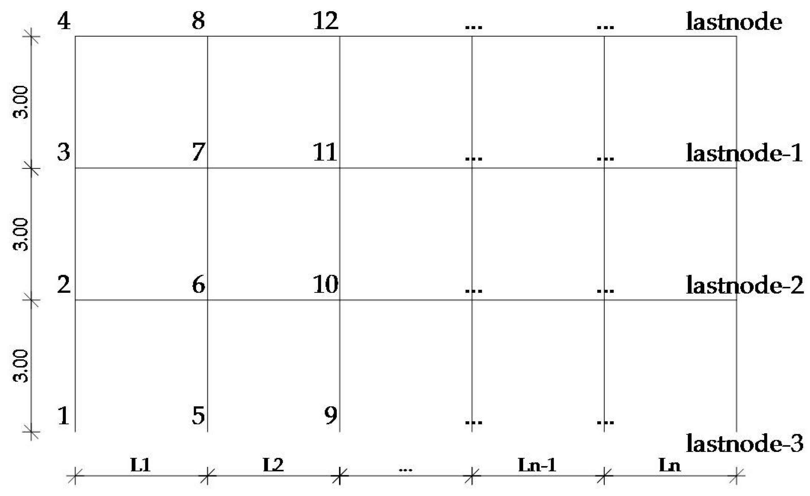
Figure 2.
Simulation of the interaction diagram of Nrd and Mrd.
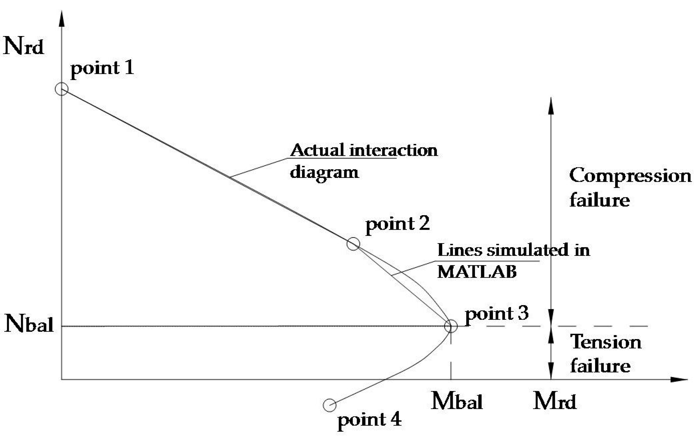
Table 1.
Loading and number of storeys considered for the first frame with a length equal to 15 m.
| Number of Storeys | Loading | Loading | Loading | Loading | Length of Frame |
|---|---|---|---|---|---|
| 2 | 15 kN/m | 35 kN/m | 55 kN/m | 75 kN/m | 15 m |
| 3 | 15 kN/m | 35 kN/m | 55 kN/m | 75 kN/m |
Table 2.
Loading and number of storeys considered for the second frame with a length equal to 25 m.
| Number of Storeys | Loading | Loading | Loading | Loading | Length of Frame |
|---|---|---|---|---|---|
| 2 | 15 kN/m | 35 kN/m | 55 kN/m | 75 kN/m | 25 m |
| 3 | 15 kN/m | 35 kN/m | 55 kN/m | 75 kN/m |
Table 3.
Loading and number of storeys considered for the third frame with a length equal to 35 m.
| Number of Storeys | Loading | Loading | Loading | Loading | Length of Frame |
|---|---|---|---|---|---|
| 2 | 15 kN/m | 35 kN/m | 55 kN/m | 75 kN/m | 35 m |
| 3 | 15 kN/m | 35 kN/m | 55 kN/m | 75 kN/m |
© 2017 by the authors. Licensee MDPI, Basel, Switzerland. This article is an open access article distributed under the terms and conditions of the Creative Commons Attribution (CC BY) license (http://creativecommons.org/licenses/by/4.0/).
Share and Cite
MDPI and ACS Style
Bekas, G.K.; Stavroulakis, G.E. Machine Learning and Optimality in Multi Storey Reinforced Concrete Frames. Infrastructures 2017, 2, 6. https://doi.org/10.3390/infrastructures2020006
AMA Style
Bekas GK, Stavroulakis GE. Machine Learning and Optimality in Multi Storey Reinforced Concrete Frames. Infrastructures. 2017; 2(2):6. https://doi.org/10.3390/infrastructures2020006
Chicago/Turabian StyleBekas, Georgios K., and Georgios E. Stavroulakis. 2017. "Machine Learning and Optimality in Multi Storey Reinforced Concrete Frames" Infrastructures 2, no. 2: 6. https://doi.org/10.3390/infrastructures2020006