
An Enhanced Algorithm for Concurrent Recognition of Rail Tracks and Power Cables from Terrestrial and Airborne LiDAR Point Clouds


Department of Geomatics Engineering, University of Calgary, 2500 University Drive NW, Calgary, AB T2N 1N4, Canada
Infrastructures 2017, 2(2), 8; https://doi.org/10.3390/infrastructures2020008
Submission received: 12 January 2017
/
Revised: 29 May 2017
/
Accepted: 31 May 2017
/
Published: 2 June 2017
(This article belongs to the Special Issue Building Information Modelling for Civil Infrastructures)
Abstract
:This study proposes an enhanced algorithm that outperforms the methods developed by the author’s earlier contributions for the recognition of railroad assets from LiDAR point clouds. The algorithm is improved by: (1) making it applicable to railroads with any slope; (2) employing Eigen decomposition for the rail seed point selection that makes it independent of the rails’ dimensions; and (3) developing a computationally efficient fully data-driven method (simultaneous identification of rail tracks and contact cables) that is able to process poorly sampled datasets with complicated configurations. The upgraded algorithm is applied to two datasets with quite different point sampling and complexity. First dataset is scanned by a terrestrial system and contains three million points covering 630 m of an inter-city railroad corridor. It presents a simple configuration with nonintersecting straight rail tracks and cables. Second dataset includes 80 m of a complex urban railroad environment comprising curved and merging rail tracks and intersecting cables. It is scanned from an airborne platform and contains 165,000 points. The results indicate that all objects of interest are identified and the average recognition precision and accuracy of both datasets at the point cloud level are greater than 95%.
1. Introduction
As-built model generation of civil infrastructures is a topic of interest in both academia and industry. Railroad corridors, buildings, roadways, and tunnels are some instances of civil infrastructure whose modeling information provides very useful information. Such 3D models can be employed for construction progress monitoring (for project management), displacement and deformation analysis (maintenance applications), and for future design refinement [1]. This study proposes an automated methodology for recognition of railroad assets from LiDAR data, which can be employed for generating modeling information of railroad environments as one of the primary civil infrastructures.
Railroad corridors are monitored to ensure they provide a safe environment for trains in motion. Safety of railroad environment is of great importance considering that rail transportation constitutes a large portion of passenger travel and freight around the globe. In Japan, for instance, more than 22 billion passengers use the rail transportation annually. The American and Russian freight rail make up to 42% and 65% of their total freight, respectively [2]. Currently, railroad corridors are monitored manually by staff traversing along the corridors to identify problematic eco-systems and potential defects in the rail infrastructure. Broken rails (29%) and equipment failure (13%) are the second and third leading causes of the rail accidents, respectively, after human factor (38%) [3].
The manual investigation of railroad environment is quite slow-paced, costly, and error prone due to human mistakes. Scanning the railroad corridors with mobile laser scanning (MLS) systems provide an accurate three-dimensional (3D) representation of the current state of such environments. MLS systems are typically composed of multiple light detection and ranging (LiDAR) sensors, a global navigation satellite system (GNSS), an inertial navigation system (INS), and sometimes digital photo/video cameras [4]. The LiDAR sensors of MLS systems scan the surrounding environment in two-dimensional (2D) profiles along trajectory of the moving train and the acquired data contains 3D points in the coordinate system of the LiDAR sensor at data collection time [5]. The captured point clouds are then integrated with the navigation data acquired by GNSS and INS and the resulting data is in the form of registered point clouds in a national or global coordinate system. MLS systems provide very fast data collection with quite precise measurements. They are mounted on either terrestrial platforms (such as trains) or airborne platforms (like helicopters). However, the volume of MLS data is often quite large and its processing is computationally very intense. Automated processing of MLS data is absolutely crucial to employ such cutting-edge remote sensing technology. This study presents an enhanced algorithm with better performance than the methods proposed in the author’s earlier contributions [6,7]. Herein, the algorithm is improved so that it is able to successfully classify very low sampled railroad point clouds with quite complicated configuration. The algorithm enhancement is elaborated in detail in the last paragraph of Section 2. Figure 1 demonstrates a sample railroad corridor and the associated elements. The key elements are shown by arrows and are fully described by Arastounia [6] and briefly in the following.
- Track bed is the surface beneath rail tracks and is topped with ballast, which holds rail tracks in line and on surface. The ballast consists of sized solid particles that are able to handle tamping and drain well [8]. Although track bed is not an essential component of railroad corridors, it indicates the areal extent of such environments.
- Rail tracks consist of two parallel steels with I-beam cross sectional profile. They come in pairs and provide a stable platform for trains in motion. Rails’ dimensions and gauge (the spatial offset between a pair of rails) follow a national or regional standard so that the railroad corridors of a country or a continent can be interconnected. The European standard gauge is 1.435 m and its rail height ranges from 0.142 m to 0.172 m [8].
- Masts are vertical poles that are located in regular spatial offset on track bed. They are either wooden or metal and hold the overhead cables in place.
- Overhead cables comprise contact cables and catenary cables. Contact cables appear as linear-shaped objects that transmit power to trains. They lie in the lowest height among all overhead cables. Catenary cables are curvilinear-shaped objects that are located immediately above contact cables and keep the contact cables in place. Contact and catenary cables are interconnected by thin plastic tubes called droppers. Catenary cables are also connected to masts by metal tubes called cantilevers. The classification of droppers and cantilevers do not fit in the scope of this work though.
2. Literature Review
Many studies have worked on the extraction and modeling of objects from LiDAR data. Estefanik et al. [9] create digital terrain model (DTM) from airborne LiDAR data. Jochem et al. [10] and Wu et al. [11] extract buildings from LiDAR data of urban environments. Yu et al. [12] identify road features from mobile terrestrial LiDAR datasets. Hullo et al. [13] create as-built model of industrial sites from terrestrial LiDAR data. Fang et al. [14] extract trees from airborne LiDAR point clouds. Arastounia [1] generates as-built model of subway tunnels from mobile terrestrial LiDAR data.
The following reviews the most recent and relevant studies in object extraction from railroad corridor point clouds. Morgan [15] visually inspects MLS data of railroad corridors to detect potential defects in the assets. Leslar et al. [16] create 3D model of rail tracks from terrestrial MLS data. Soni et al. [17] extract rail tracks from static MLS point clouds. However, the studies in [15,16,17] use manual methods. Some studies employ integrated sources of data to reconstruct rail tracks’ centerline such as Beger et al. [18] who use airborne MLS data integrated with extremely high resolution ortho-images. The rail track masks are derived by applying edge-detection algorithms to ortho-images and rail tracks are then recognized by using the spatial information provided by the rail track masks. Beger et al. [18] enhance the methodology proposed by Neubert et al. [19] in which pre-classified data are required. Sawadisavi et al. [20] use image processing techniques to detect irregularities and defects in wood-tie fasteners, rail anchors, crib ballast and turnout components. Defects in the aforementioned components do not introduce a serious danger to the moving trains though. Zhu and Hyyppa [21] recognize urban features such as terrain, roads, buildings, and trees in the surrounding of a railroad corridor. They integrate airborne and terrestrial MLS data; convert the integrated data into images; and apply image processing techniques. However, the main elements of railroad environment such as rail tracks are not recognized in this work.
Arastounia [6] recognizes key components of a railroad corridor from very well sampled terrestrial MLS data with a rather simple setup. Although all objects of interest are recognized, the performance of the algorithm deteriorates for poorly sampled data such as datasets utilized in this contribution. Arastounia [6] investigates the entire dataset’s local neighborhoods in order to detect the rail tracks, which imposes a significant computational load (taking roughly 3 h). Arastounia and Oude Elberink [7] improved the computational efficiency of the rail track extraction by coarsely classifying all of the data based on points’ height into three clusters from which the rail tracks, contact, and catenary cables are identified. The rough classification is based on the assumption that the vertical spatial offsets among the railroad assets are constant throughout the entire dataset. This assumption holds for the most parts of the urban rail corridors but it may not be the case in rural rail corridors such as mountainous areas whose track bed may experience a large slope. Herein, in order to identify “only the seed points” of the rails and cables (and not all points), the coarse classification is applied to a very small portion of the data in which the height difference among rail assets are certainly constant, due to safety regulations. This not only enhances the algorithm’s computational efficiency even more (as it only takes less than 5 min for each dataset in this work, compared to 3 h in Arastounia [6]), it also makes the algorithm applicable to both rural and urban railroad corridors with any slope angle. Furthermore, Arastounia [6] and Arastounia and Oude Elberink [7] utilize the points’ height variance and height variation for the detection of rail seed points, respectively, which both need the precise rail height. However, this work employs the Eigen decomposition for this purpose, which makes it independent of the rails dimensions. Moreover, Arastounia [6] presents a sequential algorithm in which recognition of objects of interest is carried out separately and is highly dependent on each other. That is, first, track bed is extracted and masts, cantilevers, and cables are then sequentially identified, implying that a failure in recognition of an object leads to failure in detection of the remaining objects. Arastounia and Oude Elberink [7] employ a model-driven (template matching) methodology to eliminate the false positives. Even though their proposed template matching algorithm is quite effective for the false positive removal, it is still a model-driven approach that is computationally more intense than data-driven methods. Herein, a fully data-driven (region growing) algorithm is developed that simultaneously recognizes a pair of rails and the overhead contact cable, which takes advantage of basic characteristics of rail tracks and cables for their identification. That is rail tracks always appear as a pair of rails that are parallel and are within a fixed spatial offset from one another and a contact cable always appears above a rail track as well. The introduction of these two constraints plays a major role in excluding false positives while enhancing the computational efficiency, since it is a fully data-driven algorithm. Employing this fully data-driven approach decreased the computational time from about 5 h in Arastounia and Oude Elberink [7] to less than 30 min in this work. In summary, the algorithm is enhanced by:
- Investigation of “only a small portion” of data to identify track bed in order to enhance the computational efficiency from 3 h in Arastounia [6] to less than 5 min in this study.
- Limiting the application of the coarse classification algorithm to a very small portion of the data, which makes the algorithm applicable to rail corridors with any slope angle.
- Modification of the rail seed point selection (by employing Eigen decomposition) in order to make it independent of the rails’ dimensions.
- Simultaneous recognition of the rail tracks and contact cables by a fully data-driven algorithm that takes advantage of the following two constraints. As a result, the false positives are successfully eliminated without imposing a notable computational burden. This decreased the computational time from approximately 5 h in Arastounia and Oude Elberink [7] to less than 30 min in this contribution.
- Rail tracks always appear as a pair of rails that are parallel and have an invariable spatial offset from one another.
- There is one contact cable above each rail track.
The author’s previous contributions [6,7] utilize LiDAR point clouds captured only from terrestrial platforms. This contribution, in addition to employing a terrestrial point cloud, also tests the developed algorithm on an airborne LiDAR point cloud (see Section 3.2) with the lowest sampling and most complicated configuration among all datasets employed in the author’s earlier contribution in [6,7].
3. Datasets
3.1. Terrestrial LiDAR Point Cloud
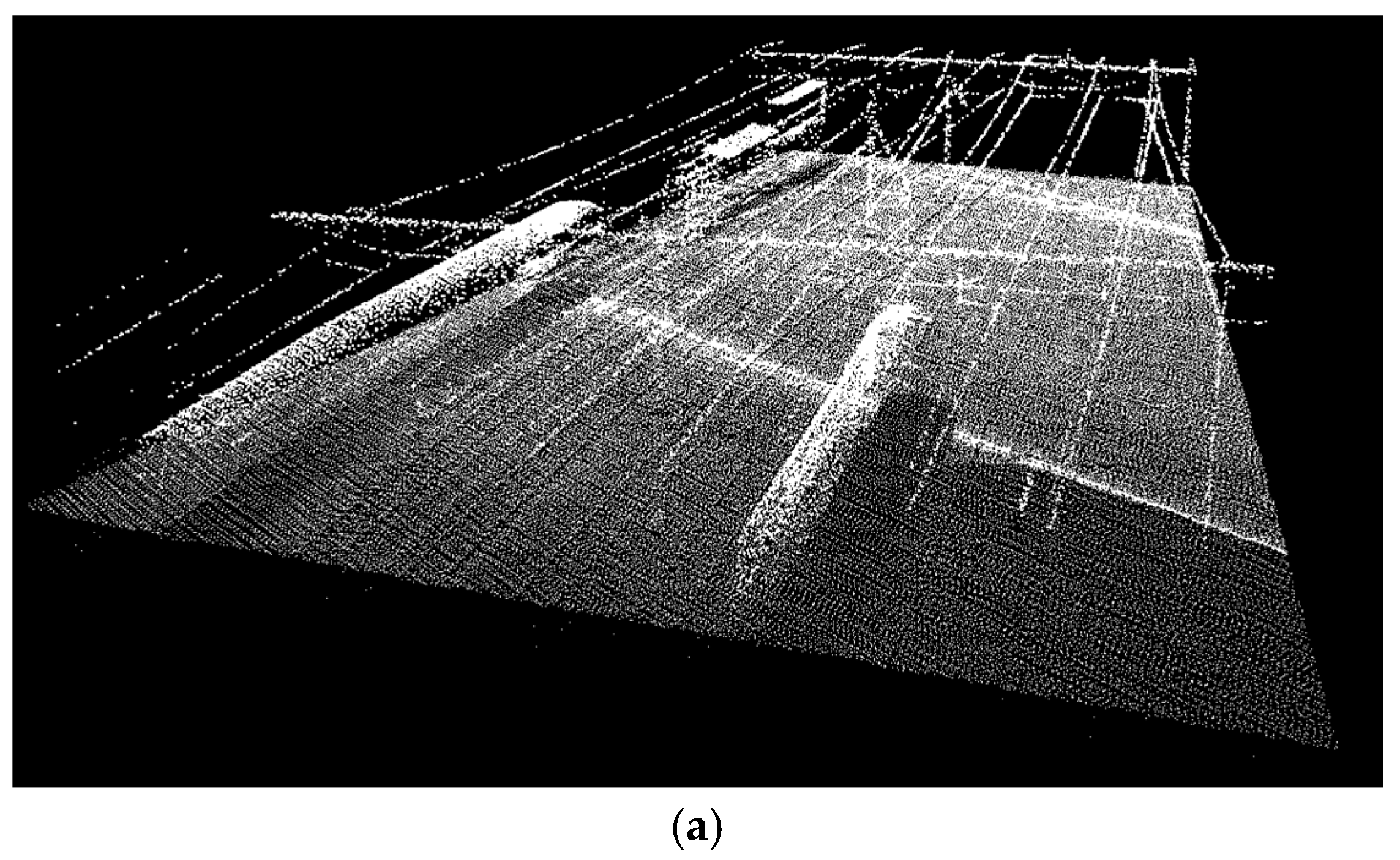
The first dataset covers 630 m of Dutch inter-city railroad corridors near the city of Elst including two rail tracks (four rails), two contact cables and two catenary cables. In addition to the railroad elements, it includes points belonging to the surrounding environment such as train stations, humans, masts, trees, etc. This dataset with more than three million (3,079,210) points contains only geometrical information (points’ 3D coordinates) with no intensity and no RGB data. The points are in the Dutch national coordinate system and their precision is at millimeter level. Figure 2a indicates the dataset from an oblique view and Figure 2b shows a finer representation of the railroad assets. As is evident in this figure, masts are located in regular spatial intervals (approximately 67 m); catenary cables lie immediately above contact cables; and cables intersect with masts.
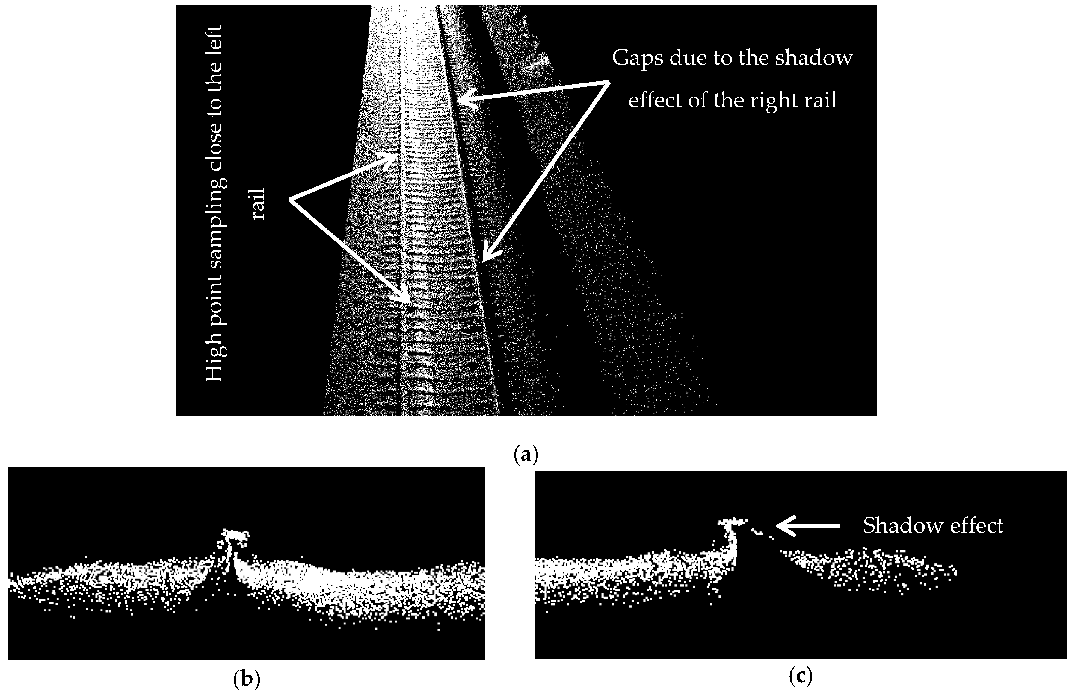
The point sampling is quite fluctuant in different parts of the dataset, especially on track bed. Figure 3 indicates the non-uniform point sampling on different parts of the track bed. Figure 3a indicates that the sampling close to the left rail is much higher than that of the right rail. This is also evident in Figure 3b,c in which the left rail is well scanned while the right rail is partially scanned due to its shadow effect. Figure 3a also shows that there are large gaps (areas with no points) due to the rails’ shadow effect. The sampling of contact cables is almost twice as dense as that of the catenary cables due to their shorter spatial offset from LiDAR sensors.
3.2. Airborne LiDAR Point Cloud
The second dataset is collected by a fast laser imaging mapping and profiling (FLI-MAP 400) system, which is an airborne laser scanning (ALS) system used for mobile and area mapping. FLI-MAP 400 is a helicopter-based system that is able to map 100–200 linear km per day in corridor mapping applications and 50–100 km2 per day in area mapping applications. It consists of a LiDAR sensor, a line-scan camera, two digital high resolution photo cameras, two fixed-focus digital video cameras, a GNSS and an INS [22]. Table 1 presents the specifications of the LiDAR sensor of a FLI-MAP 400 system.
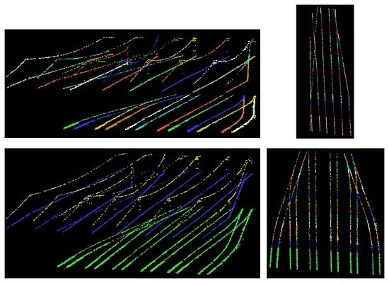
The dataset covers about 80 m of a railroad corridor close to the main train station of Enschede, a city in the east of the Netherlands and it only contains points belonging to the railroad infrastructure including eight rail tracks (sixteen rails), nine contact cables and nine catenary cables (Figure 4a). The points belonging to the surrounding environment are removed by data collection staff. The dataset contains 164,640 points with only points’ 3D coordinates and no auxiliary source of information and the coordinates’ precision is at centimeter level. Although the size of this dataset seems a little small, it contains a very challenging part of the railroad environment due to its complex configuration and poor sampling. As is evident in Figure 4b,c, it incorporates both straight and curved rail tracks, straight and curved cables, merging rail tracks and intersecting cables. Moreover, the point sampling is quite poor due to the long spatial offset between the railroad assets and the LiDAR sensor on helicopter. This can be best visualized in Figure 4d, in which the rail’s cross sectional shape is hardly recognizable. Figure 4e demonstrates the track bed’s fluctuant point sampling, which is due to different scanning pattern and the presence of external objects on track bed. Furthermore, the average point sampling of the railroad assets are presented in Table 2 that indicates the sampling of the first dataset is much higher than that of the second dataset. The sampling of cables and track bed in the first dataset are almost four and seven times as dense as those in the second dataset, respectively. Track bed sampling in both datasets is also much higher than that of cables due to the track bed’s larger dimensions.
4. Methodology
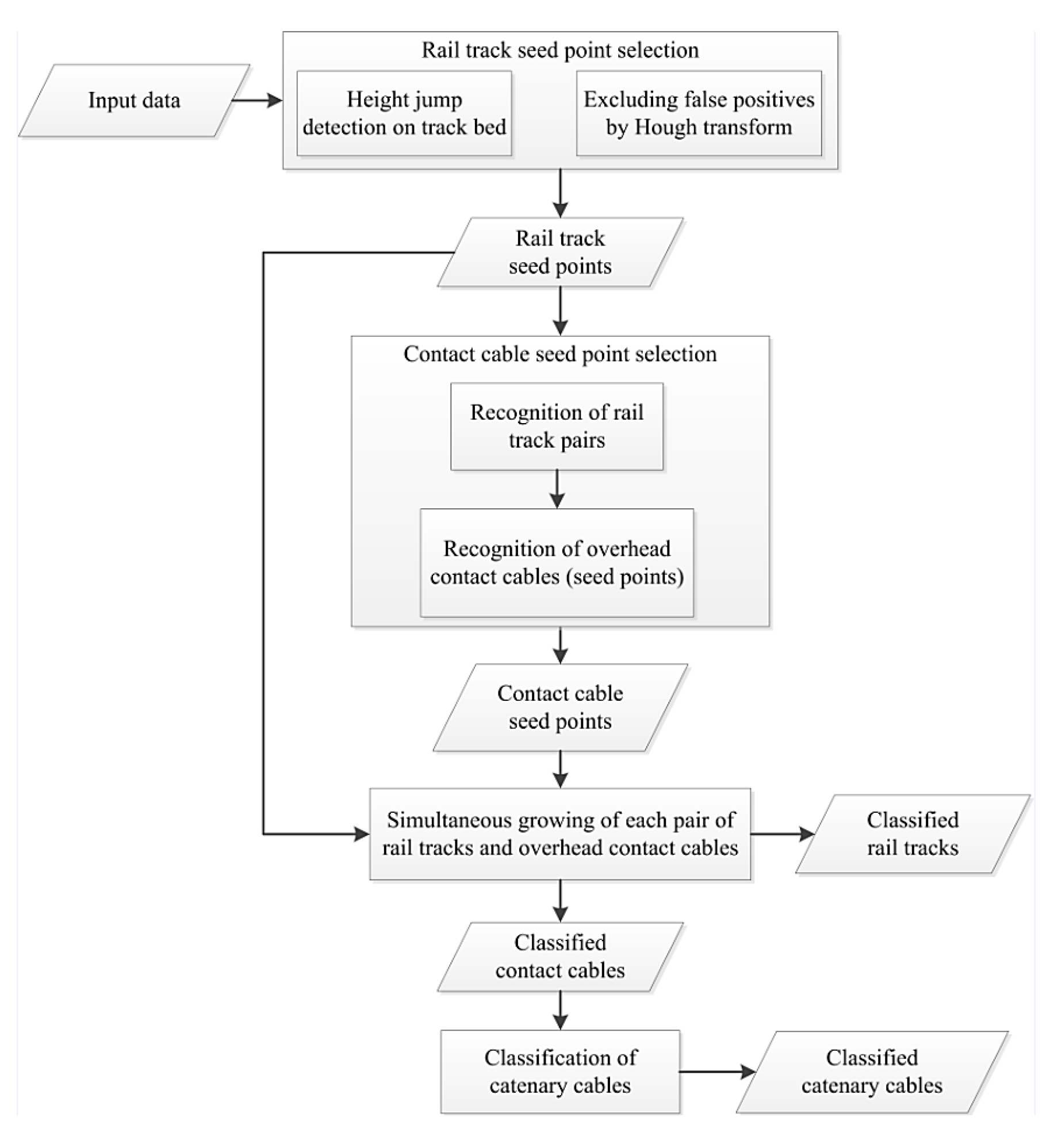
The proposed algorithm is composed of two main parts. First, points belonging to the rail tracks and contact cables are concurrently recognized in Section 4.1 and points belonging to the catenary cables are then identified in Section 4.2. Figure 5 presents the flowchart of the developed methodology.
4.1. Simultaneous Recognition of Rail Tracks and Contact Cables
The rail tracks and contact cables are identified by applying a region growing algorithm. First, a small portion of the data is roughly classified in Section 4.1.1. Section 4.1.2 and Section 4.1.3 then describe the selection criteria for the rail track and contact cable seed points, respectively. The similarity measures employed for the region growing are explained in Section 4.1.4.
4.1.1. Classification Based on Height
First, a coarse classification based on points’ height that is proposed by Arastounia and Oude Elberink [7] is applied to a small portion of the dataset. It is required to note that Arastounia and Oude Elberink [7] applied the rough classification to the entire dataset, assuming the vertical spatial offset among the railroad assets are constant throughout the entire dataset. Although this is the case for the most parts of the urban rail corridors, it may not be the case at all times, especially in mountainous areas where the track bed might have a large slope. Herein, this method is applied for such a small portion of the dataset in which the height difference between the rail tracks and over-head cables certainly remains constant, due to safety restrictions. Considering the point sampling of the employed datasets in this work, the selected portion covers five and fifteen meters of the rail corridor in the first and second dataset, respectively, so that there would be adequate number of points to provide reliable information regarding the centroid location, average height, and distribution direction of rail tracks and cables.
The coarse classification aims to separate points belonging to objects of interest from one another and group them in different clusters. It is based on points’ height and the fact that there is a certain vertical offset among rail tracks and overhead cables. Track bed has the largest dimensions among all railroad components and yet has a very low height variation. Thus, the most common height in the selected small portion of the data represents the track bed height. That being said, points within half a meter higher or lower than track bed are gathered in the first cluster; points within five meters to five and half meters above track bed are aggregated in the second cluster; and points higher than five and half meters above track bed are grouped in the third cluster. The first, second, and third clusters are hereinafter referred to as low-height, medium-height, and top-height clusters, respectively. As a result, points belonging to the rail tracks, contact cables and catenary cables are aggregated in low-height, medium-height, and top-height cluster, respectively. These three clusters are expected to incorporate points belonging to other objects such as other railroad equipment, trees, and humans, which are not of interest in this work. Therefore, only the first two clusters are further processed to identify points belonging to rail tracks out of low-height cluster (constituting rail seed points) and extract points belonging to contact cables out of medium-height cluster (forming contact cable seed points).
4.1.2. Rail Seed Point Selection
The rail seed points are selected by applying Eigen decomposition to the points belonging to the low-height cluster, obtained from Section 4.1.1. To that end, the covariance matrix of each point’s local neighborhood is constructed as in Equation (1), in which denote the variance and covariance along the respective cardinal directions, respectively. Next, the eigenvalues and eigenvectors are calculated by the principal component analysis (PCA) [23], as in Equation (2), in which represent the covariance matrix, matrix of eigenvalues, matrix of eigenvectors, and an identity matrix, respectively. Considering the covariance matrix size, PCA calculates three eigenvalues () and three eigenvectors () for each local neighborhood. Each eigenvalue () indicates the dispersion magnitude of the neighborhood under inspection along the associated eigenvector (). By assuming , and denote the query neighborhood’s direction of the largest and smallest dispersion.
Given that the track bed is constructed to have the smallest height variation possible in longitudinal direction, due to the safety regulations, the smallest eigenvalue () of a local neighborhood without a piece of rail is nominally zero-valued and a neighborhood containing a piece of rail has a non-zero eigenvalue. However, due to the covering material of the track bed (ballast) that forms a non-flat surface and the presence of inevitable noise in the data, parts of the track bed even without a piece of rail indicate a very small height variation, which makes its smallest eigenvalue () slightly larger than zero. That being said, all local neighborhoods of low-height cluster whose smallest eigenvalue () satisfies the condition in Equation (3) are marked as containing a piece of rail. Then, points higher than 90th height percentile within each local neighborhood (that was identified to contain a piece of a rail) are labeled as belonging to rail tracks.
False positives are anticipated due to presence of the external objects on track bed that might induce height variations as large as rails. Such false positives are excluded by applying 2D Hough transform [24] to the labeled rail points. Hough transform detects points lying on the same line and also computes parameters of the respective line. Herein, each line represents a rail and its parameters correspond to the orientation direction and 3D coordinates of centroid of the rail under inspection. Therefore, points belonging to each rail and the rail’s orientation direction and centroid location are obtained by applying Hough transform. The labeled points that are not identified by Hough transform are considered as false positives and are discarded.
The pseudocode of the rail seed point selection is presented below:
- Notation: : points identified as belonging to track bed in Section 4.1.1; : a sample point; : 3D spherical local neighborhood of a sample point; : covariance matrix of a sample point’s local neighborhood; : eigenvalues; : 90th height percentile of a query neighborhood; : a sample point’s height; : points lying higher than 90th height percentile within a query point’s neighborhood; : lines obtained from applying Hough transform; : a segment containing rail seed points.
- Input:
- for
- Find
- Construct
- Calculate eigenvalues of by applying PCA to
- if then
- Compute of
- for
- ○
- if then
- ○
- ○
- end if
- end for //loop on
- end if //condition on
- end for //loop on
- Calculate by applying 2D Hough transform to
- for
- if then
- end if //condition on
- end for //loop on .
4.1.3. Contact Cable Seed Point Selection
Considering that rail tracks always appear as a pair of rails, the algorithm starts by recognition of rail pairs using rail seed points identified in the previous section. As is evident in Figure 6, the rails of a pair are parallel and are spaced apart by the gauge size. Thus, if two rails are parallel (Equation (4)) and the 2D Euclidean distance between their centroids has a maximum deviation of 0.05 m (rail width) from gauge size (Equation (5)), they are deemed as belonging to the same pair. In Equations (4) and (5), and Ci denote the orientation direction and centroid of a rail, respectively. The symbol indicates the angle between two vectors and X and Y denote points’ coordinates.
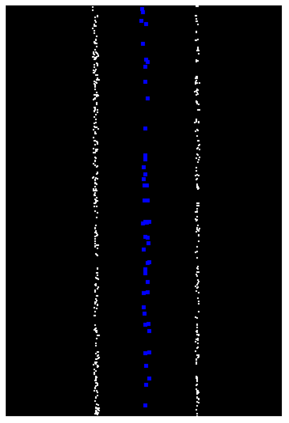
Once rail pairs are recognized, points belonging to each pair of rails and points of medium-height cluster are projected into planimetric plane and points of medium-height cluster that are within one meter 2D Euclidean distance of rail pairs are labeled as contact cable seed points. That is since contact cables lie above rail tracks and appear as linear objects between two rails of a pair in planimetric view (Figure 7). Next, contact cable seed points that lie within one meter 3D Euclidean distance of one another are aggregated in segments until no more seed points are left. The average height and orientation direction of each segment is then calculated. Consequently, the rail pairs and the overhead contact cables in the selected small portion of rail corridor are identified as seed points for the region growing.
The pseudocode of the contact cable seed point selection is provided in the following.
- Notation: : segments containing seed rail points obtained from Section 4.1.2; : points belonging to medium-height cluster obtained from Section 4.1.1; : number of (rail) pair segments; : a sample segment; : covariance matrix of points belonging to a sample segment; : eigenvector corresponding to the largest eigenvalue of points belonging to ith segment; : centroid of the ith segment; : the angle between two vectors; : planimetric distance between two points; : the rail pair segment; : the cable seed segment.
- Input: and
- Set
- for
- Construct and
- Calculate of by applying PCA to
- Calculate of by applying PCA to
- Calculate and
- if (() and ()) then
- ○
- Set
- ○
- ○
- ○
- for
- ○
- if () then
- ○
- ○
- end if
- ○
- end for //loop on
- end if
- end for //loop on and .
4.1.4. Region Growing
The recognition of railroad infrastructure is pursued by simultaneous growing of each pair of rails and the above contact cable. To that end, points within a certain neighborhood of a rail pair that are not yet classified and satisfy the following two conditions are considered as candidate rail points.
- The point’s height () is within 0.05 m (half rail height) of the rail segment’s average height (), as in Equation (6).
- The vector connecting the rail segment to the query point () makes a small angle with the rail segment’s orientation direction () as in Equation (7).
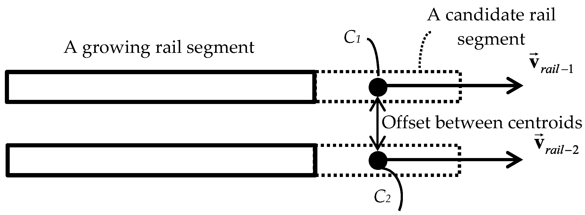
Next, candidate rail points that are within one meter 3D Euclidean distance of one another are segmented; let us call them candidate rail segments whose centroid’s (Ci) 3D coordinates and orientation direction () are then computed. If the candidate segments’ orientation directions () are parallel (as in Equation (8)) and the 2D Euclidean distance between their centroids (Ci) has a maximum deviation of 0.05 m (rail width) from gauge size (as in Equation (9)), they are considered as belonging to rail tracks and are added to the growing rail segment. Figure 8 indicates such concurrent growing of a pair of rails in which candidate rail segments are depicted by dashed rectangles and their centroids are shown by black points.
Once one meter of a pair of rails is recognized and prior to extracting the remaining of the query rail track, one meter of the overhead contact cable is identified. To this end, points within a close neighborhood of the growing contact cable segment that are not yet classified and meet the conditions in Equations (10) and (11) are considered as belonging to contact cables and are added to the growing contact cable segment. Equation (10) inspects if a point’s height () is almost within the same height of the growing segment () and Equation (11) checks whether the vector connecting the query point to the growing segment () is aligned along the growing segment (). The concurrent growing of each pair of rails and the overhead contact cable is pursued until no point within their close neighborhood meets the above-mentioned conditions. The height and orientation direction of the growing rail pairs and the overhead contact cables are updated after each step of growing. Once a rail track and the overhead contact cable is fully grown, the growing is pursued for the next rail pair (rail track) and its overhead contact cable until all pairs are entirely grown.
The orientation direction vectors in Equations (7), (8), and (11) are computed by applying the Eigen decomposition to the points belonging to the growing rail segment, candidate rail segment, and growing contact cable segment, using Equations (1) and (2). The eigenvector () corresponding to the largest eigenvalue () represents the principal orientation direction [23]. One should note that as was mentioned in Section 4.1.2, the orientation direction vectors in Equation (4) are calculated by Hough Transform. Furthermore, the angle threshold () in Equations (4), (7), (8), and (11) is selected based on rail tracks’ smooth curvature gradient [8]. This along with other height and distance thresholds employed in the aforementioned equations are chosen with respect to railroad corridor specifications, which are invariable and alike in the entire railroad corridors of a country and a continent so that railroad corridors of the neighboring countries can be interconnected. The neighborhood size in the region growing algorithm is also selected regarding the point spacing of the employed datasets. Herein, one meter and five meter neighborhood sizes are considered for the first and second dataset, respectively.
It is required to note that the simultaneous growing of rail tracks and contact cables introduces two strong and effective constraints (below) and, thus, plays a major role in the successful recognition of rail tracks by excluding false positives.
- Rail tracks always appear as two parallel rails that are located within a fixed spatial offset (gauge) from one another.
- There is one contact cable above each and every rail track.
If any of the above two conditions is not met, the newly-identified piece of rail is considered as false positive and is not considered for further processing. This is not the case in Arastounia [6] in which extraction of rail tracks and overhead cables are executed separately. Such false positive removal is performed by Arastounia and Oude Elberink [7] by converting 3D points into 2D images and applying image processing techniques (template matching), which requires more intense computations than the developed algorithm in this work does.
The pseudocode of the region growing algorithm is presented in two parts in order to provide a convenient read. The first part indicates the clustering of two candidate rail segments of a rail pair and the second part presents the growing of a rail pair and atop cable. This procedure (pseudocode below) is pursued for all rail pairs until no more points meet the criteria in Equations (6) to (11).
- Notation: : a pair of growing rail segments obtained from Section 4.1.2; : two rail segments belonging to a growing rail pair; : average height of the ith growing rail segment; : principal distribution direction of the ith growing rail segment; : local neighborhood of the ith growing rail segment; : a sample point; : vector connecting a sample point to the growing rail segment; the ith candidate rail segment.
- Input:
- for
- Calculate and
- Compute and
- Find and
- for
- Calculate
- if (() and ()) then
- end if //condition on and
- end for //loop on
- for
- Calculate
- if (() and ()) then
- end if //condition on and
- end for //loop on
- end for //loop on and .
The pseudocode above showed how candidate rail segments were clustered and the code below indicates how the segments containing a rail pair and the cable atop are grown.
- Notation: : ith candidate rail segment belonging to a rail pair; : points belonging to cable seed segments obtained from Section 4.1.3; : principal distribution direction of the ith candidate rail segment; Ci: centroid of the ith candidate rail segment; : the angle between two vectors; : planimetric distance between two points; : average height of the growing contact cable above a rail pair; : principal distribution of the growing contact cable above a rail pair; : local neighborhood of the growing cable segment; : a sample point; : vector connecting a sample point to the growing contact cable segment; : points belonging to the growing rail segment; points belonging to the growing contact cable segment.
- Input: , , and
- Calculate and
- Calculate C1 and C2
- if (() and () ) then
- Calculate
- Compute
- Find
- for
- Calculate
- ○
- if (() and () ) then
- ○
- ○
- ○
- ○
- end if
- end for //loop on
- end if.
4.2. Classification of Catenary Cables
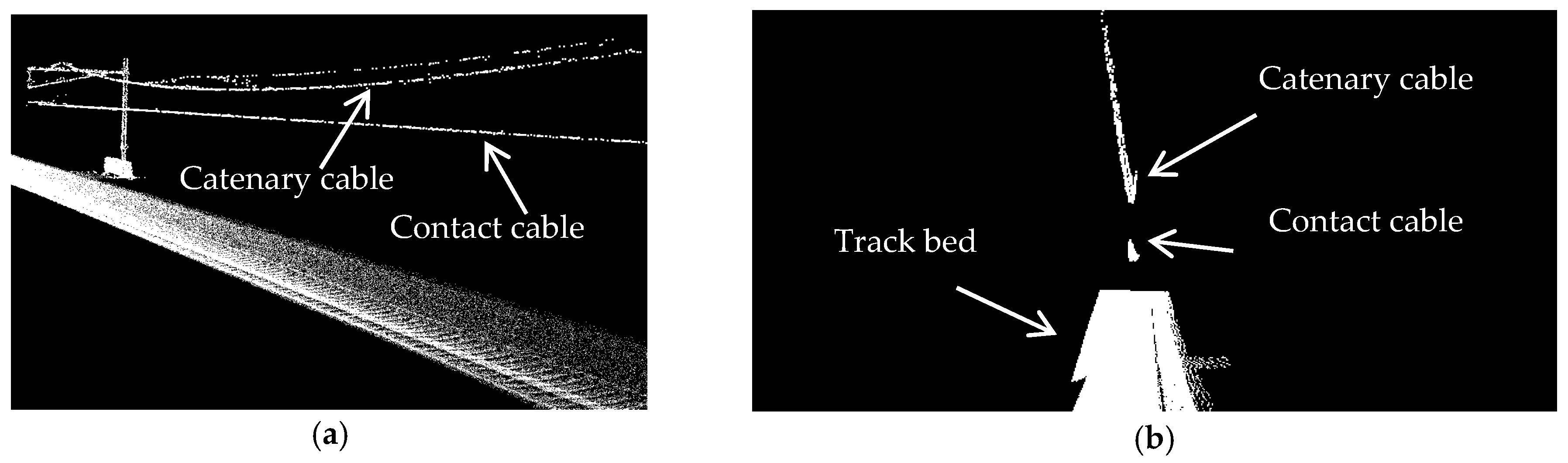
Catenary cables are the only objects that lie immediately above contact cables and there are no other objects in such a close neighborhood of contact cables (Figure 9). Therefore, the points belonging to the catenary cables are identified by seeking for points that meet both of the following two conditions.
- Lie higher in elevation than a point belonging to the contact cables.
- Located within 0.2 m 2D spatial offset from either side of the same contact cable point.
Afterwards, the labeled points that are within one meter neighborhood of one another are clustered. The distance threshold (0.2 m) used in this section is chosen based on the cables’ dimensions and the topological relationship between them. One needs to note that some false positives are expected at the intersections of cables with one another and with masts.
The pseudocode of catenary cable recognition is as follows:
- Notation: : points belonging to contact cables identified in Section 4.1.4; : points belonging to top-height cluster obtained from Section 4.1.1; : a sample point; : points belonging to contact cables that are within 0.2-m planimetric distance of a query point belonging to top-height cluster; : a sample point’s height; : segment containing points belonging to catenary cables.
- Input: and
- for
- Find
- for
- if then
- end if
- end for //loop on
- end for //loop on .
5. Results and Discussion
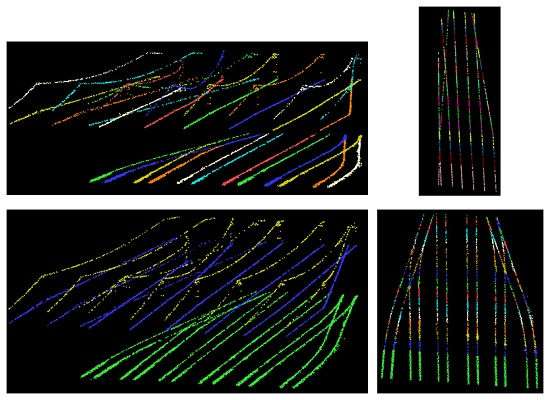
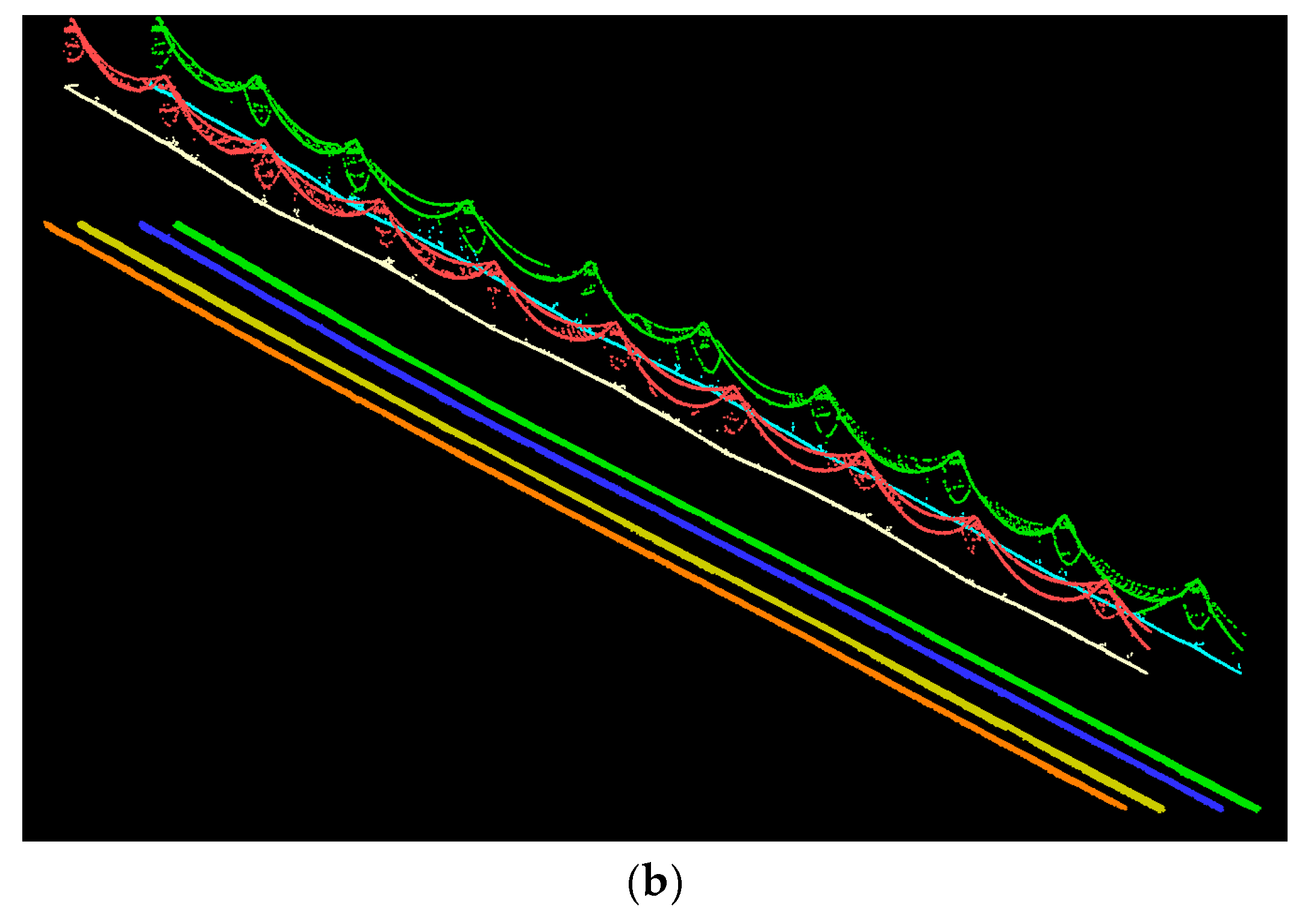
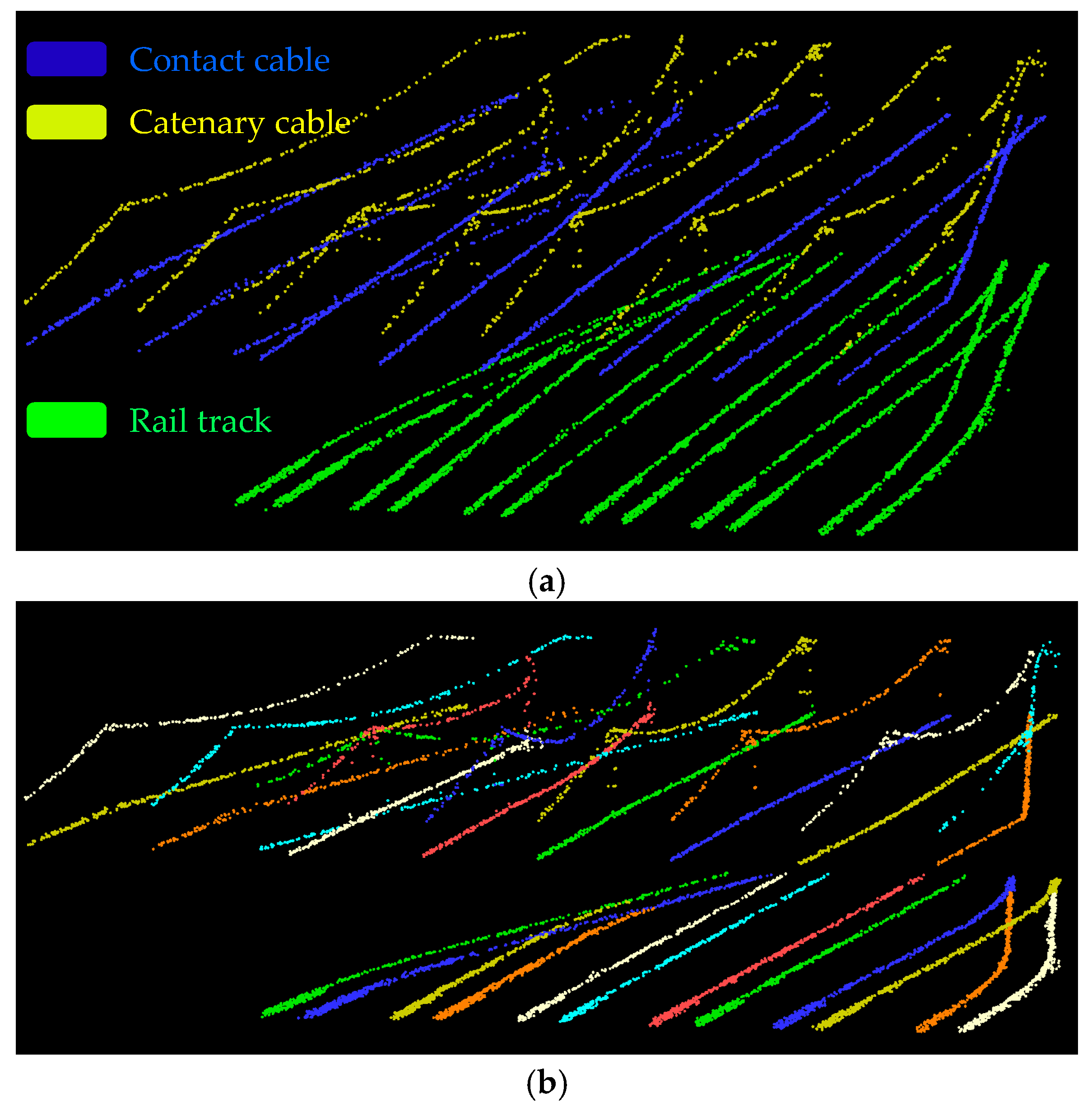
Figure 10a,b demonstrates the first dataset’s region growing results with one-meter growing step and Figure 10c,d shows the results of the second dataset with five-meter growing step. The large segments at the bottom of these four figures indicate the seed points and other parts represent the growing steps. Figure 11a and Figure 12a indicate the classification results based on object type in which each type of object is depicted in a different color. Figure 11b and Figure 12b show that each object is separately classified and shown in a different color.
The obtained results are evaluated at the object and point cloud level in terms of classification precision and accuracy. Points belonging to the objects of interest were manually cropped and saved as ground truth data, which were then employed to calculate the precision and accuracy at point cloud level using the following formulas.
where represent true positive, false positive, true negative and false negative, respectively. Precision provides the percentage of relevant results and a perfect (100%) precision score implies that all points that are recognized by the algorithm as belonging to a certain object indeed belong to that object. Accuracy is the arithmetic mean of precision and inverse precision that provides a measure to assess the algorithm’s ability to both identify points belonging to the objects of interest and excluding points that do not belong to the objects of interest. A perfect (100%) accuracy score suggests that the algorithm was able to identify all points belonging to the objects of interest without including any point belonging to objects that are of no interest. All objects of interest in both datasets are successfully classified with no false positives and no false negatives, which corresponds to 100% accuracy and 100% precision at the object level. The achieved results at the point cloud level are also presented in Table 3 in terms of classification precision and accuracy.
The non-perfect classification results of rail tracks are due to false positives, gaps and poorly sampled areas in the datasets. False positives are primarily induced by small external objects and railroad equipment on the track bed. Although the majority of false positives are successfully excluded, a few of them that are located very close to rails are not eliminated. Gaps and poorly sampled areas are also introduced by large external objects (such as rail cars) on the track bed. Figure 13 indicates the external objects and poorly sampled areas in two datasets. Figure 13a demonstrates two external objects and the associated poorly sampled areas in the first dataset and Figure 13b depicts a locomotive, three large rail cars and the resulting low sampled areas in the second dataset. According to Table 3, the precision and accuracy of rail track classification in the first dataset is slightly (about 3%) higher than those in the second dataset, suggesting that rail track classification in the first dataset is more successful than that in the second dataset. That is since the track bed sampling in the first dataset is seven times as dense as that in the second dataset (Table 2). This is also confirmed by Figure 3b,c that shows rail tracks in the first dataset are very well scanned and their cross sectional shape can be conveniently recognized, whereas the rail track sampling in the second dataset is so poor that their cross sectional shape cannot even be visualized (Figure 4d). Furthermore, the rail tracks configuration in the second dataset is much more complex with sixteen curved, straight and merging rails while the first dataset comprises only four non-merging straight rails. External objects also have a bigger negative impact on the second dataset since they induce four large poorly sampled areas (totally 288 m2) in the second dataset, whereas they introduce one small low sampled area (13 m2) in the first dataset.
The contact cable classification in the first dataset was quite successful as it reached a very high (greater than 99%) precision and accuracy at the point cloud level. Their high point sampling has a key role in their successful classification in the first dataset. They are well sampled since the first dataset was acquired from a terrestrial platform and consequently there was a short spatial offset between LiDAR sensor and contact cables. Their unique (piece-wise linear) shape, topological relationship with other objects and sparse configuration also had a great impact in achieving such good results. However, their sparse configuration is specific to the first dataset and is not necessarily the case for other datasets. Contact cable classification measures in the second dataset are slightly (about 2%) lower than those of the first dataset due to their lower sampling and more complicated setup. Their point sampling in the first dataset is almost four times as dense as that in the second dataset (see Table 2) and their complex configuration with many intersections is evident in Figure 14.
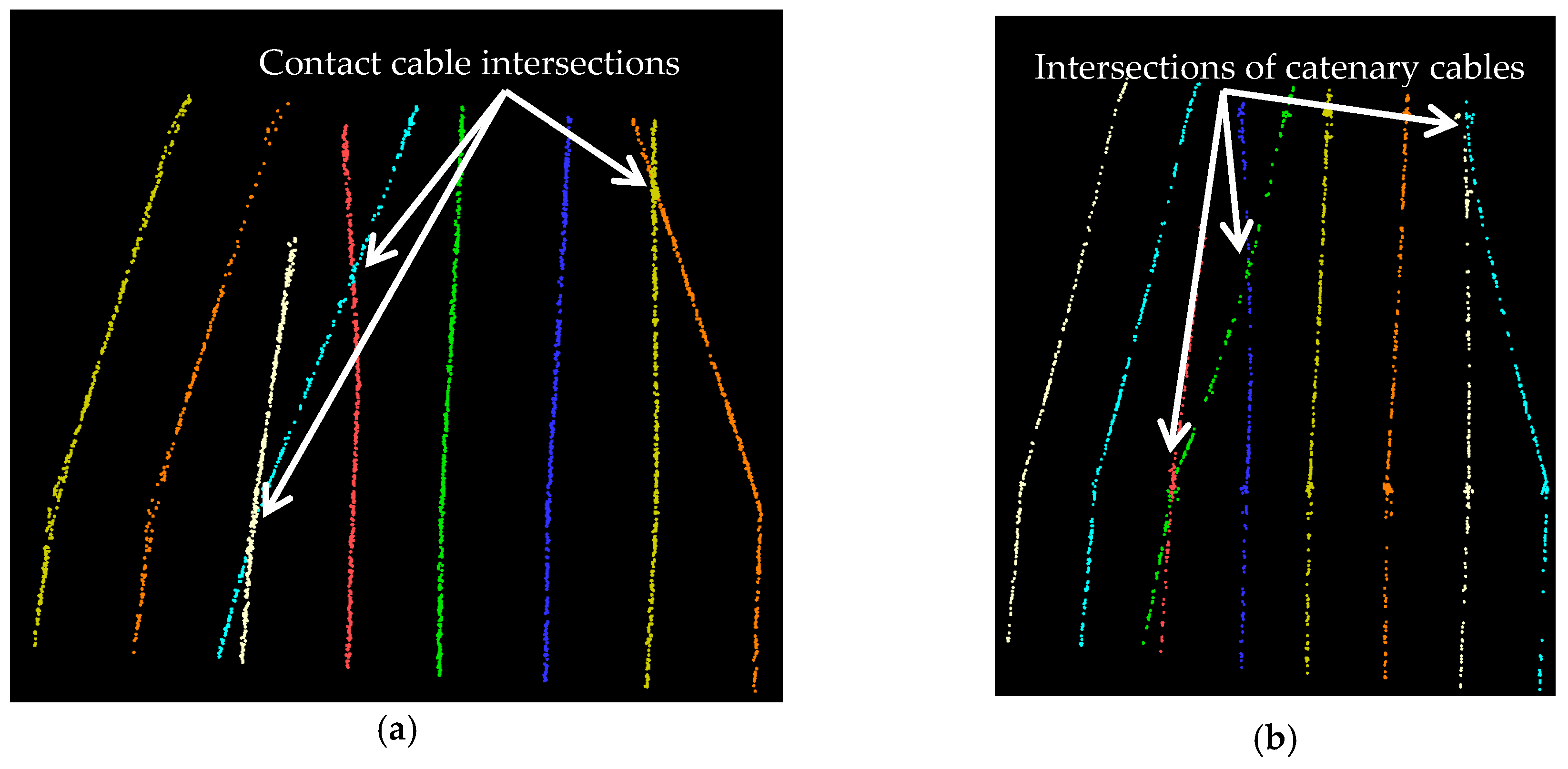
The catenary cable classification measures in both datasets are also quite high (greater than 95%). In contrast to other objects, the catenary cable’s precision in the second dataset is marginally higher than that in the first dataset due to false positives at their intersections with masts in the first dataset. There are ten such intersections in the first dataset while there is only one such intersection in the second dataset. Few false positives in the second dataset took place at three intersections of catenary cables with one another (Figure 14b). The classification accuracy of catenary cables in both datasets is quite high due to their unique topological relationship with contact cables. That is they are the only object immediately above contact cables and there are no other objects in such a close neighborhood of contact cables.
The employed datasets in this study are quite different from one another so that the developed algorithm’s performance on datasets with different configuration and point sampling is tested. The first dataset includes a rather simple configuration with two straight rails, two nonintersecting contact and two nonintersecting catenary cables. The sampling of the objects of interest in this dataset is also very high. However, there are many urban features in these data such as humans, building facades, lampposts and trees, which makes the classification more challenging. On the other hand, the second dataset presents a quite intricate setup with curved, straight and merging rail tracks and intersecting cables. The sampling of this dataset is also so poor that the rails’ physical shape is hardly recognizable (Figure 4d). However, it only includes railroad components with no points belonging to the surrounding environment. That being said, the very high classification accuracy and precision (greater than 95%) of two datasets imply that the algorithm is able to handle datasets with different point sampling and configuration.
Since both terrestrial and airborne MLS data are employed in this work, the following briefly discusses the merits and shortcomings of these systems for such mobile mapping applications. Terrestrial MLS systems typically provide higher point sampling due to their shorter spatial offset from objects, compared to airborne systems. They are also a more suitable choice for scanning railroad corridors that go through underground tunnels or dense forests where airborne systems are either inapplicable or unable to perform well due to occlusion of the tree crowns. However, employing ALS systems can profoundly increase the safety of railroad environments since defects in railroad assets (such as a broken rail) can be identified from ALS data before a train reaches to the problematic area. ALS systems also provide faster data collection since their platform (helicopter) is usually faster than terrestrial platforms (trains). Additionally, although the sampling of ALS data is usually lower than that of terrestrial systems, it is more uniform due to similar spatial offset between the LiDAR sensor and various objects.
6. Conclusions
This study presents an improved algorithm that outperforms the methods proposed by the author’s earlier contributions in [6,7] for the recognition of rail tracks, contact cables, and catenary cables from railroad corridor point clouds. The algorithm enhancement in this work includes: (1) applying the coarse classification (based on height) only to a small portion of data in order to make it applicable to railroads with any slope; (2) using Eigen decomposition for the rail seed point selection that is able to work regardless of the rails’ dimensions; and (3) developing and applying a fully data-driven method (concurrent recognition of rail tracks and contact cables) that allows for a computationally efficient processing of poorly sampled datasets with complicated configurations. The simultaneous detection of the rail tracks and contact cables is based on their very basic characteristics that rail tracks always appear as a pair of parallel rails within a fixed distance from one another, which are topped with a contact cable. This is verified since the upgraded algorithm successfully classifies a very poorly sampled airborne dataset with a quite complex setup (described Section 3.2), whereas the algorithms presented in the author’s previous contributions in [6,7] achieve poor results on this dataset. The presented methodology also employs only 3D coordinates of points with no need for auxiliary sources of data such as imagery or intensity. Two datasets of Dutch railroad corridors are used in this work. The first dataset is captured by a terrestrial MLS system and covers 630 m of four rails, two contact cables and two catenary objects. It contains more than three million points and has a simple configuration with non-merging straight rail tracks and nonintersecting cables. The second dataset is collected by an airborne MLS system and covers 80 m of sixteen rails, nine contact cables and nine catenary cables. The second dataset with about 165,000 points has a very complex configuration incorporating curved, straight and merging rail tracks and intersecting cables. The results show that 100% precision and 100% accuracy at the object level in both datasets are achieved. At the point cloud level, the contact cables reach the highest precision and accuracy (99%) in the first dataset due to their high sampling and isolated position. These measures of rail tracks and catenary cables in this dataset are also quite high (95%). In the second dataset, the catenary cables obtain the best result due to their isolated position and simpler setup. The overall results of the first dataset are slightly (2%) better than those of the second dataset due to its higher sampling and less complex configuration. The high average precision and accuracy (greater than 95%) of both datasets indicate that the proposed methodology is able to handle datasets with different point sampling and configuration while preserving high computational efficiency.
Acknowledgments
Fugro Geo-Services and Movares are greatly acknowledged for data acquisition.
Conflicts of Interest
The author declares no conflict of interest.
References
- Arastounia, M. Automated as-built model generation of subway tunnels from mobile LiDAR data. Sensors 2016, 16, 1486. [Google Scholar] [CrossRef] [PubMed]
- American Public Transportation Association. Available online: http://www.apta.com/resources/statistics/Documents/FactBook/2014-APTA-Fact-Book.pdf (accessed on 16 May 2015).
- USA Federal Railroad Administration. Available online: http://safetydata.fra.dot.gov/OfficeofSafety/publicsite/Query/AccidentByRegionStateCounty.aspx (accessed on 11 January 2015).
- Petrie, G. Mobile mapping systems: An introduction to the technology. GeoInformatics 2010, 13, 32–43. [Google Scholar]
- Kutterer, H. Mobile Mapping. In Airborne and Terrestrial Laser Scanning, 1st ed.; Vosselman, G., Maas, H.-G., Eds.; Whittles Publishing: Caithness, UK, 2010; pp. 293–295. [Google Scholar]
- Arastounia, M. Automated recognition of railroad infrastructure in rural areas from LiDAR data. Remote Sens. 2015, 7, 14916–14938. [Google Scholar] [CrossRef]
- Arastounia, M.; Oude Elberink, S. Application of template matching for improving classification of urban railroad point clouds. Sensors 2016, 16, 2112. [Google Scholar] [CrossRef] [PubMed]
- Bianculli, A.J. Track: Introduction. In Trains and Technology; University of Delaware: Newark, DE, USA, 2003; pp. 60–95. [Google Scholar]
- Stefanik, K.V.; Gassaway, J.C.; Kochersberger, K.; Abbott, A. UAV-based stereo vision for rapid aerial terrain mapping. GISci. Remote Sens. 2013, 48, 24–49. [Google Scholar] [CrossRef]
- Jochem, A.; Hofle, B.; Rutzinger, M.; Pfeifer, N. Automatic roof plane detection and analysis in airborne Lidar point clouds for solar potential assessment. Sensors 2009, 9, 5241–5262. [Google Scholar] [CrossRef] [PubMed]
- Wu, B.; Yu, B.; Wu, Q.; Yao, S.; Zhao, F.; Mao, W.; Wu, J. A graph-based approach for 3D building model reconstruction from airborne LiDAR point clouds. Remote Sens. 2017, 9, 92. [Google Scholar] [CrossRef]
- Yu, Y.; Li, J.; Guan, H.; Wang, C. Automated extraction of urban road facilities using mobile laser scanning data. IEEE Trans. Intell. Transp. Syst. 2015, 16, 2167–2181. [Google Scholar] [CrossRef]
- Hullo, J.F.; Thibault, G.; Boucheny, C.; Dory, F.; Mas, A. Multi-sensor as-Built models of complex industrial architectures. Remote Sens. 2015, 7, 16339–16362. [Google Scholar] [CrossRef]
- Fang, F.; Im, J.; Lee, J.; Kim, K. An improved tree crown delineation method based on live crown ratios from airborne LiDAR data. GISci. Remote Sens. 2016, 53, 402–419. [Google Scholar] [CrossRef]
- Morgan, D. Using mobile LiDAR to survey railway infrastructure. In Proceedings of the Innovative Technologies of Efficient Geospatial Management of Earth Resources, Lake Baikal, Listvyanka, Russia, 23–30 July 2009. [Google Scholar]
- Leslar, M.; Perry, G.; McNease, K. Using mobile LiDAR to survey a railway line for asset inventory. In Proceedings of the ASPRS 2010 Annual Conference, San Diego, CA, USA, 26–30 April 2010. [Google Scholar]
- Soni, A.; Robson, S.; Gleeson, B. Extracting rail track geometry from static terrestrial laser scans for monitoring purposes. In Proceedings of the ISPRS Technical Commission V Symposium, Riva del Garda, Italy, 23–25 June 2014. [Google Scholar]
- Beger, R.; Gedrange, C.; Hecht, R.; Neubert, M. Data fusion of extremely high resolution aerial imagery and LiDAR data for automated railroad center line construction. ISPRS J. Photogramm. Remote Sens. 2011, 66, 40–51. [Google Scholar] [CrossRef]
- Neubert, M.; Hecht, R.; Gedrange, C.; Trommler, M.; Herold, H.; Kruger, T.; Brimmer, F. Extraction of rail road objects from very high resolution helicopter-borne LiDAR and ortho-image data. In Proceedings of the Geographic-Object-Based Image Analysis (GEOBIA) 2008, Calgary, AB, Canada, 5–8 August 2008. [Google Scholar]
- Sawadisavi, S.; Edwards, J.R.; Resendiz, E.; Hart, J.; Barkan, C.P.L.; Ahuja, N. Machine-vision inspection of railroad track. In Proceedings of the American Railway Engineering and Maintenance-of-Way Association (AREMA) 2008 Annual Conference, Salt Lake City, UT, USA, 21–24 September 2008. [Google Scholar]
- Zhu, L.; Hyyppa, J. The use of airborne and mobile laser scanning for modelling railway environments in 3D. Remote Sens. 2014, 6, 3075–3100. [Google Scholar] [CrossRef]
- Fugro Geo-Services LTD. Available online: http://www.fugro.ca/services/aerial-survey/flimap/flimap400/ (accessed on 21 May 2016).
- Jolliffe, I.T. The Singular Value Decomposition. In Principal Component Analysis, 2nd ed.; Springer Series in Statistics: New York, NY, USA, 2002; pp. 44–47. [Google Scholar]
- Hough, P.V.C. Method and Means for Recognizing Complex Patterns. U.S. Patent 3069654, 18 December 1962. [Google Scholar]
Figure 1.
A sample railroad corridor in which the key elements are depicted by arrows.
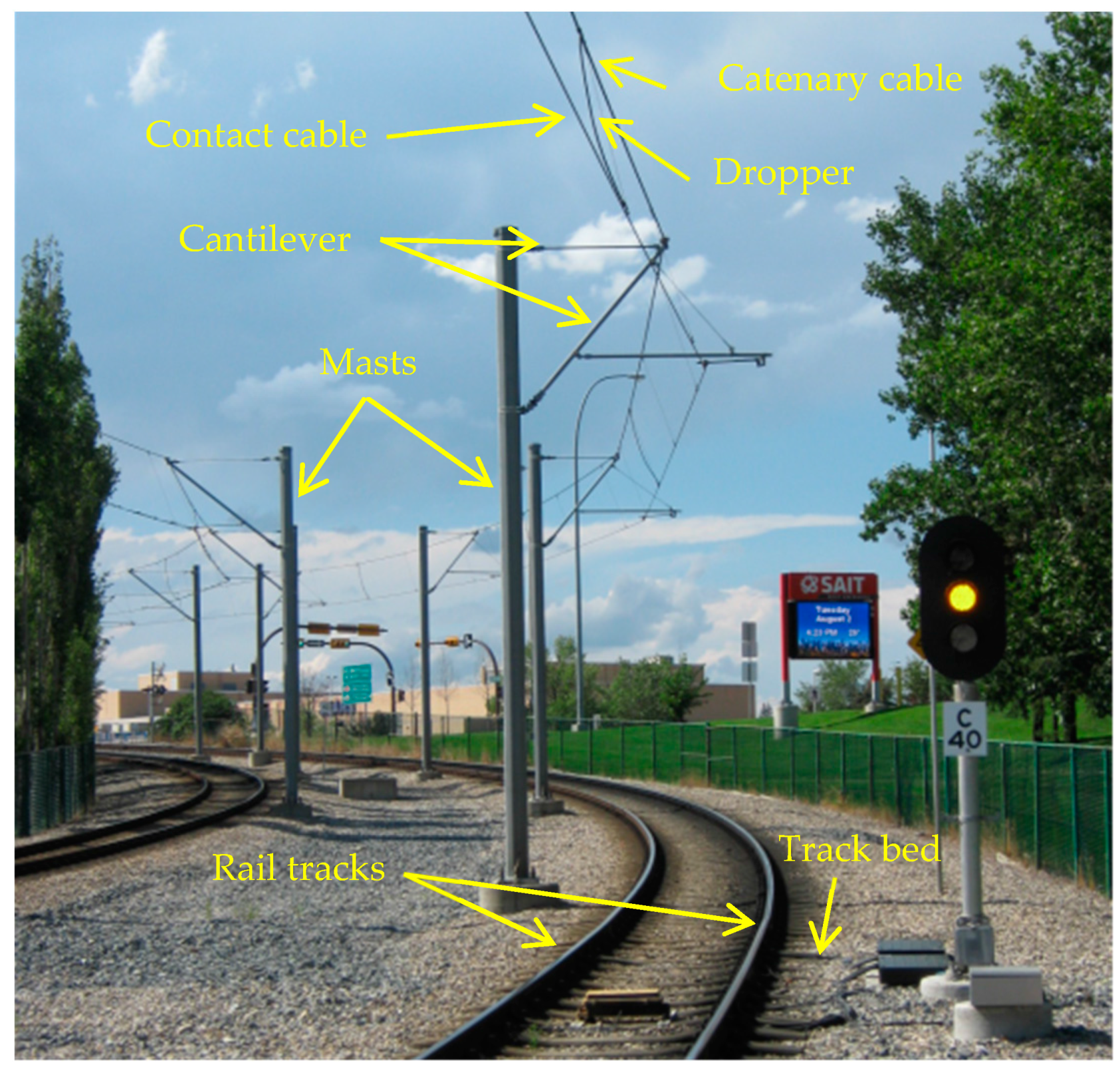
Figure 2.
First dataset: (a) The entire dataset in an oblique view; and (b) a fine representation of the key elements.
Figure 2.
First dataset: (a) The entire dataset in an oblique view; and (b) a fine representation of the key elements.
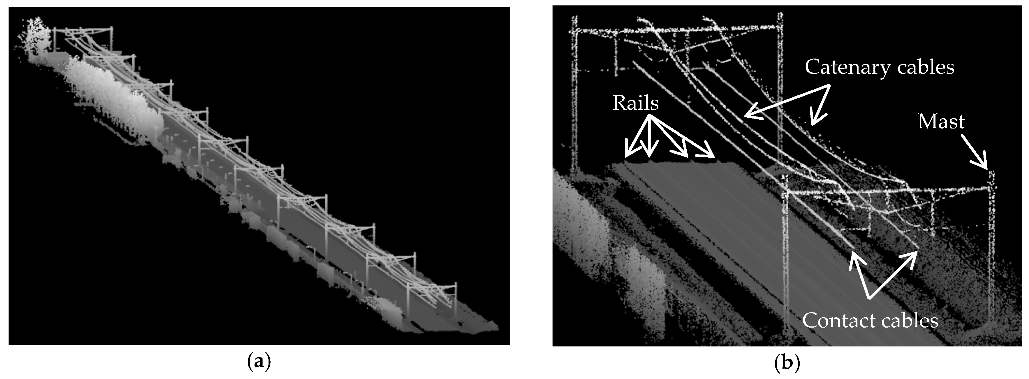
Figure 3.
Non-uniform point sampling on different parts of track bed in the first dataset: (a) The sampling close to the left rail is much higher than that of other parts of the track bed. There are also some gaps (areas with no points) due to the rails’ shadow effect. (b) The left rail is well sampled and its shape is conveniently recognizable. (c) The right rail is partially scanned due to its shadow effect.

Figure 4.
Second dataset: (a) The entire dataset in which there are some rail cars on track bed; (b) complex configuration with intersecting cables; and (c) curved and merging rail tracks; (d) rails’ cross sectional shape is hardly recognizable due to poor sampling; and (e) track bed’s sampling is quite fluctuant.

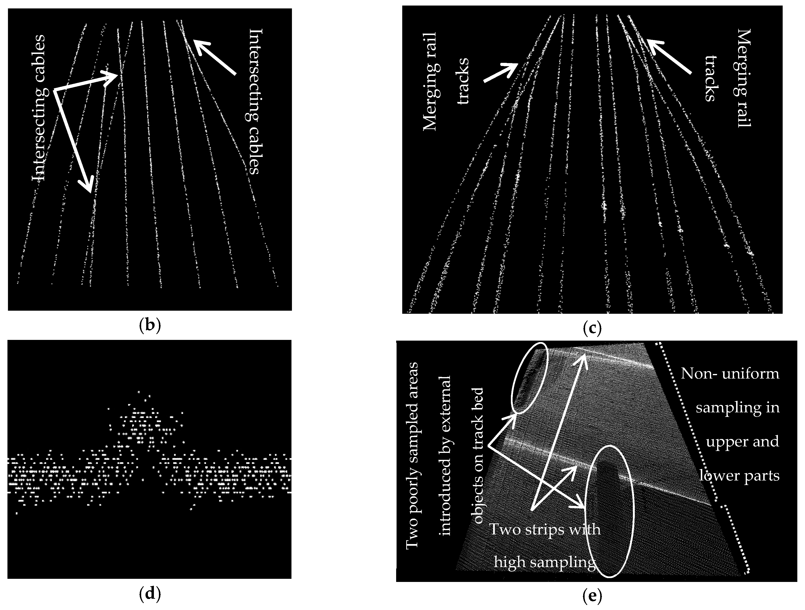
Figure 5.
Flowchart for the recognition of rail tracks and overhead cables.

Figure 6.
Two rails belonging to the same pair (in planimetric view) that are parallel and are spaced apart by the gauge size. The dashed arrows ( and ) and black points (Ci and Cj) represent the rails’ orientation direction and centroid, respectively.
Figure 6.
Two rails belonging to the same pair (in planimetric view) that are parallel and are spaced apart by the gauge size. The dashed arrows ( and ) and black points (Ci and Cj) represent the rails’ orientation direction and centroid, respectively.
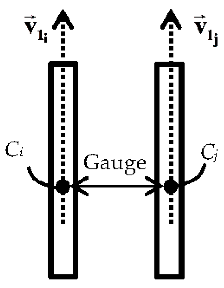
Figure 7.
Contact cables (blue points) lie above rail tracks (white points) and appear as straight linear objects between two rails in planimetric view.
Figure 7.
Contact cables (blue points) lie above rail tracks (white points) and appear as straight linear objects between two rails in planimetric view.

Figure 8.
Simultaneous growing of a pair of rails based on the orientation direction () and centroids (Ci) offset of candidate rail segments.
Figure 8.
Simultaneous growing of a pair of rails based on the orientation direction () and centroids (Ci) offset of candidate rail segments.

Figure 9.
Topological relationship between overhead cables: (a) Side view; and (b) front view of a railroad corridor indicating that catenary cables lie immediately above contact cables and there are no other objects in such a close neighborhood of contact cables.
Figure 9.
Topological relationship between overhead cables: (a) Side view; and (b) front view of a railroad corridor indicating that catenary cables lie immediately above contact cables and there are no other objects in such a close neighborhood of contact cables.

Figure 10.
Region growing results of two datasets in which large parts at the bottom indicate the seed points and other parts represent the growing steps: (a) region growing results of rail tracks; (b) contact cables in the first dataset; (c) region growing results of rail tracks; and (d) contact cables in the second dataset.
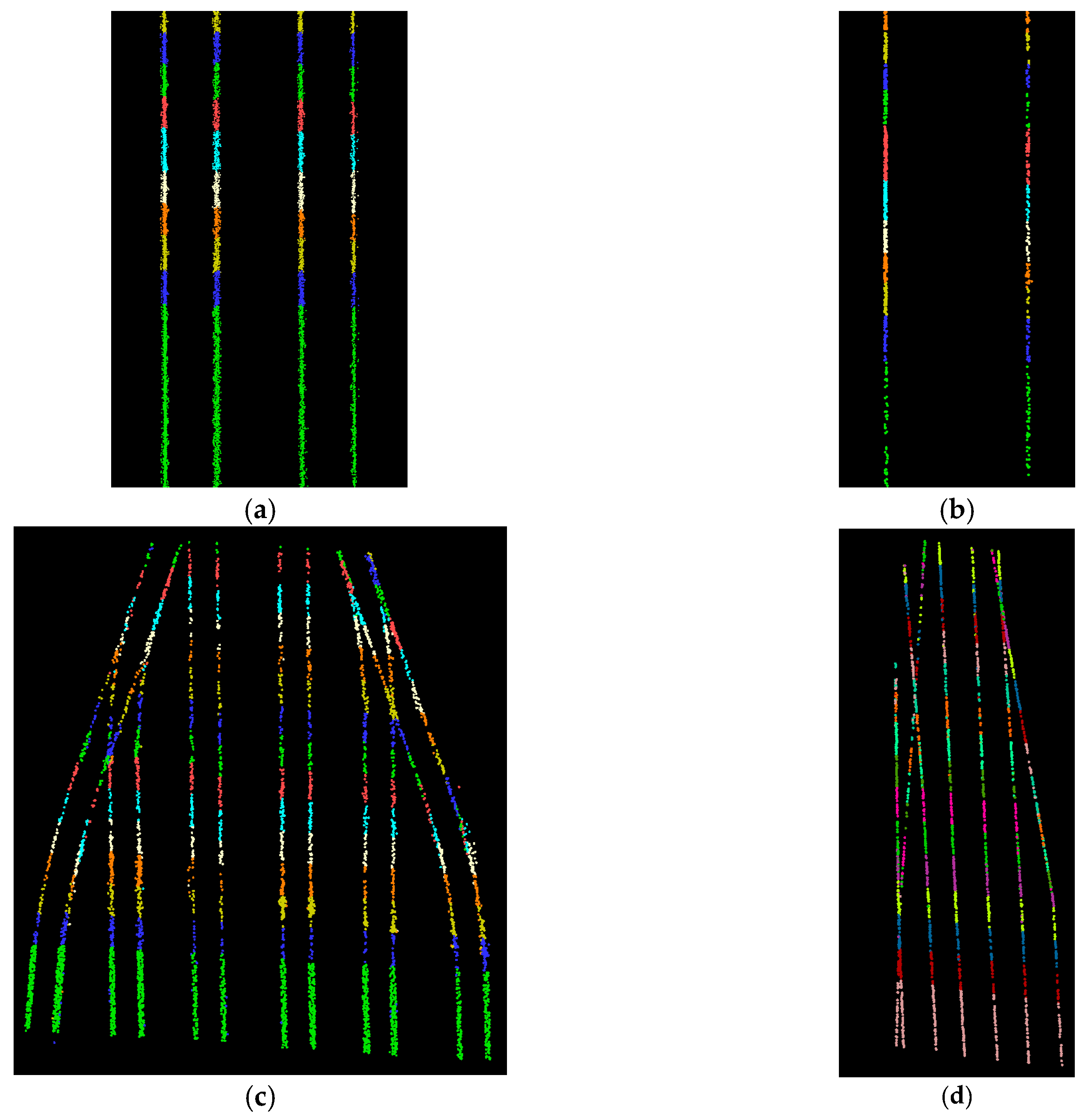
Figure 11.
Classification results of the first dataset: (a) objects of interest are classified based on their type and each type of object is shown in a different color; and (b) each object is separately recognized and shown in a different color, regardless of its type.
Figure 11.
Classification results of the first dataset: (a) objects of interest are classified based on their type and each type of object is shown in a different color; and (b) each object is separately recognized and shown in a different color, regardless of its type.
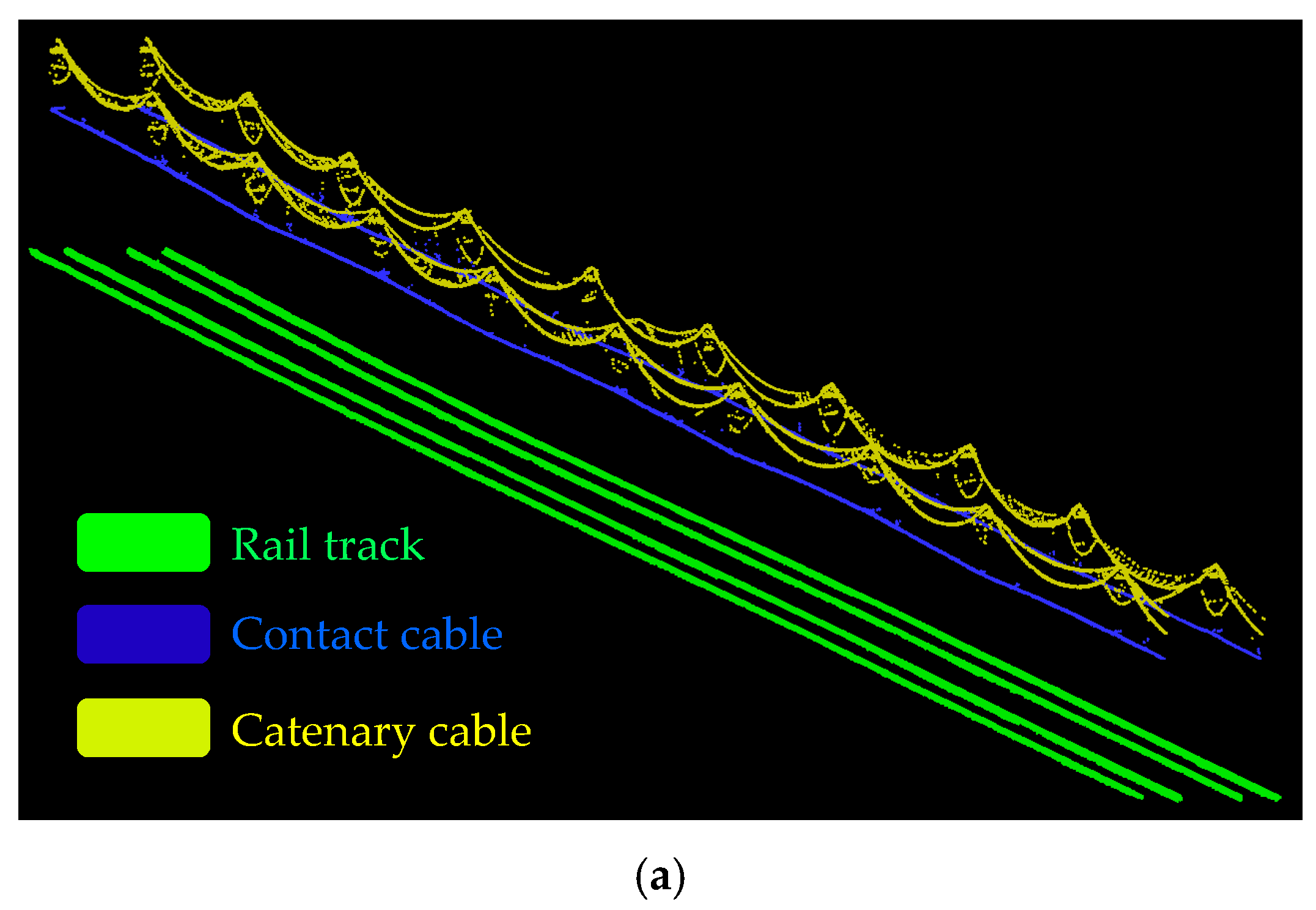

Figure 12.
Classification results of the second dataset: (a) classification results according to the object type; and (b) objects are separately classified and each object is indicated in a different color.
Figure 12.
Classification results of the second dataset: (a) classification results according to the object type; and (b) objects are separately classified and each object is indicated in a different color.

Figure 13.
Poorly sampled areas introduced by the external objects’ shadow effect: (a) in the first dataset; and (b) in the second dataset. The points belonging to the rail cars are shown in red for a convenient visualization.
Figure 13.
Poorly sampled areas introduced by the external objects’ shadow effect: (a) in the first dataset; and (b) in the second dataset. The points belonging to the rail cars are shown in red for a convenient visualization.
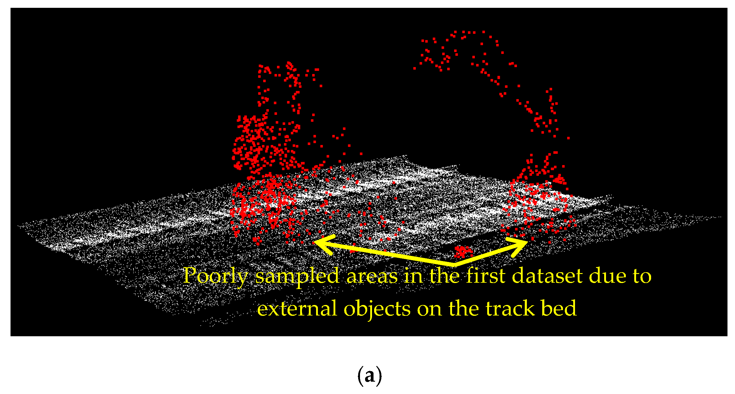
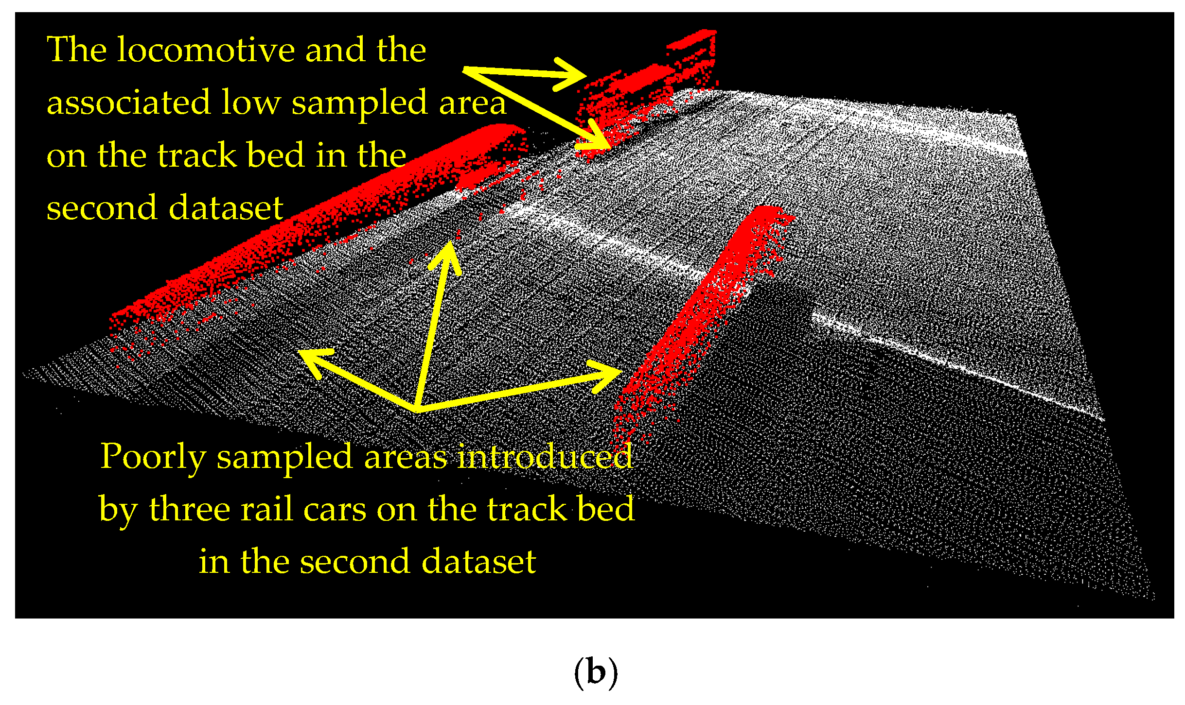
Figure 14.
False positives in second dataset at the intersections of: (a) contact cables; and (b) catenary cables.
Figure 14.
False positives in second dataset at the intersections of: (a) contact cables; and (b) catenary cables.


Table 1.
Technical Specifications of the LiDAR Sensor of a FLI_MAP 400 System.
| Specifications | Values |
|---|---|
| Laser pulse rate | 150,000 pulses per second |
| Laser eye safety | FDA certified class 1 laser (eye safe at the capture) |
| Nominal point density | >40 points per m2 at 150 m altitude and 75 km/h |
| Range accuracy | 0.01 m |
| Total system accuracy | 0.08 m horizontal and 0.05 m vertical at 1 sigma |
| Laser swath angle | Average 60 degrees (depends of the flying height) |
Table 2.
Average Point Sampling of Railroad Assets in Two Datasets.
| Objects | Point Sampling | |
|---|---|---|
| Terrestrial LiDAR Point Cloud | Airborne LiDAR Point Cloud | |
| Track bed (points/m2) | 570 | 82 |
| Contact cable (points/m) | 17 | 4 |
| Catenary cable (points/m) | 9 | 2.5 |
Table 3.
Classification Results of Two Datasets at the Point Cloud Level (in Percentage).
| Objects | Terrestrial Point Cloud | Airborne Point Cloud | ||
|---|---|---|---|---|
| Precision | Accuracy | Precision | Accuracy | |
| Rail tracks | 97.6 | 95.3 | 93.1 | 92.1 |
| Contact cables | 99.4 | 99.1 | 95.9 | 96.4 |
| Catenary cables | 95.3 | 98.2 | 96.8 | 97.2 |
| Average | 97.4 | 97.5 | 95.3 | 95.2 |
© 2017 by the author. Licensee MDPI, Basel, Switzerland. This article is an open access article distributed under the terms and conditions of the Creative Commons Attribution (CC BY) license (http://creativecommons.org/licenses/by/4.0/).
Share and Cite
MDPI and ACS Style
Arastounia, M. An Enhanced Algorithm for Concurrent Recognition of Rail Tracks and Power Cables from Terrestrial and Airborne LiDAR Point Clouds. Infrastructures 2017, 2, 8. https://doi.org/10.3390/infrastructures2020008
AMA Style
Arastounia M. An Enhanced Algorithm for Concurrent Recognition of Rail Tracks and Power Cables from Terrestrial and Airborne LiDAR Point Clouds. Infrastructures. 2017; 2(2):8. https://doi.org/10.3390/infrastructures2020008
Chicago/Turabian StyleArastounia, Mostafa. 2017. "An Enhanced Algorithm for Concurrent Recognition of Rail Tracks and Power Cables from Terrestrial and Airborne LiDAR Point Clouds" Infrastructures 2, no. 2: 8. https://doi.org/10.3390/infrastructures2020008