
The Potential of Active Contour Models in Extracting Road Edges from Mobile Laser Scanning Data


1
Geomatics Division, Centre Tecnològic de Telecomunicacions de Catalunya (CTTC/CERCA), 08860 Castelldefels, Spain
2
National Centre for Geocomputation, Maynooth University, Co. Kildare, Ireland
*
Author to whom correspondence should be addressed.
Infrastructures 2017, 2(3), 9; https://doi.org/10.3390/infrastructures2030009
Submission received: 18 April 2017
/
Revised: 19 July 2017
/
Accepted: 19 July 2017
/
Published: 22 July 2017
Abstract
:Active contour models present a robust segmentation approach, which makes efficient use of specific information about objects in the input data rather than processing all of the data. They have been widely-used in many applications, including image segmentation, object boundary localisation, motion tracking, shape modelling, stereo matching and object reconstruction. In this paper, we investigate the potential of active contour models in extracting road edges from Mobile Laser Scanning (MLS) data. The categorisation of active contours based on their mathematical representation and implementation is discussed in detail. We discuss an integrated version in which active contour models are combined to overcome their limitations. We review various active contour-based methodologies, which have been developed to extract road features from LiDAR and digital imaging datasets. We present a case study in which an integrated version of active contour models is applied to extract road edges from MLS dataset. An accurate extraction of left and right edges from the tested road section validates the use of active contour models. The present study provides valuable insight into the potential of active contours for extracting roads from 3D LiDAR point cloud data.
1. Introduction
Light Detection And Ranging (LiDAR) enables 3D modelling of the real-world environment by measuring the time of return of emitted light pulses. The information obtained through laser scanning systems, which use LiDAR technology, provides several benefits over conventional sources of data acquisition in terms of accuracy, resolution, attributes and automation [1,2,3]. The applicability of laser scanning systems continues to prove their worth in mapping due to their ability to provide a georeferenced set of dense LiDAR point cloud data [4,5,6]. With the potential of LiDAR technology in road management, Mobile Laser Scanning (MLS) systems can be used to capture 3D spatially-referenced information about road geometry and physical road objects. This information can assist decision makers in identifying the possible risk elements of the road, which may present safety concerns. MLS systems present a rapid, reliable and cost-effective alternative to various manual-based road safety schemes and standards for carrying out inspections along the route corridor. They can be used to record, locate and measure the road infrastructure elements on a large scale in order to schedule their maintenance in a timely and cost-effective manner. The acquired information can be used for effective management of road networks and to ensure maximum safety conditions for road users. The MLS data record a number of attributes including elevation, intensity, pulse width, range and multiple echo, all of which can be used for extracting information about the road and its features.
The methods developed for segmenting LiDAR data are based on the identification of planar or smooth surfaces and the classification of the point cloud based on its attributes [7]. Based on these methods, several approaches have been attempted over the past decade to extract road and its associated features from Airborne Laser Scanning (ALS) and MLS datasets. McElhinney et al. [8] developed an automated algorithm to extract road edges from MLS data by first estimating the LiDAR points within the vicinity of road cross-section lines, which were determined based on navigation data. In the second stage, the estimated points were analysed based on their attributes such as the slope, intensity, pulse width and proximity to vehicle information in order to extract the road edges. Ibrahim and Lichti [9] extracted street kerbs by applying morphological and derivative of the Gaussian functions to the ground points segmented from MLS data. Zhou and Vosselman [10] presented a three-step approach for extracting kerbs from ALS and MLS data in which small-height jumps were detected near the terrain surface, a sigmoidal function was fitted to mid points of the height jump and then small gaps between nearby and collinear line segments were closed. Wang et al. [11] detected kerbs edges from MLS data by estimating salient points based on projecting the distance of each point’s normal vector to the point cloud’s dominant vector in a hyperbolic tangent function space. The salient points were analysed based on their elevation, horizontal length and distance to the trajectory to extract the road edges. In more recent work, Hui et al. [12] proposed a method to extract main road centerlines from ALS data. In their method, an optimal intensity threshold was estimated using the skewness balancing algorithm; narrow roads were removed using the rotating neighbourhood algorithm; while the influence of attached areas was avoided using the hierarchical fusion and optimization algorithm. Xio et al. [13] fused the vehicle based camera and LiDAR datasets for road detection. In their approach, the hybrid Conditional Random Field (CRF) model was used to integrate the information from two sensors in a probabilistic way, and then, the model was efficiently optimised using graph cuts to estimate the road areas.
Road extraction approaches that have been developed to date fail to provide an efficient and robust solution. Most of the methods have been developed for extracting kerb edges in urban road environments where the algorithms rely on the existence of a sufficient height or slope difference between the road and kerb points. Little research has been focused on extracting edges in rural and semi-urban areas where the road edges distinguish the road surface from grass-soil. LiDAR intensity and pulse width attributes can be a useful source of information for extracting edges, which need to be thoroughly explored. In this context, active contour models present a robust segmentation approach that makes efficient use of specific information available about objects in the input data rather than processing all of the data [14]. The concept of the active contour was first introduced by [15] and has been widely used for image segmentation [16,17]. The active contour models present a great potential in terms of processing the 3D LiDAR data for objects’ segmentation. In this paper, we examine the active contours and their efficiency to extract road edges from MLS data. Section 2 provides a detailed discussion of active contours and their categorisation as parametric and geometric models. We review various active contour-based approaches that have been developed for extracting roads from LiDAR and digital imaging datasets. In Section 3, we present a case study in which an integrated version of active contour models is applied to extract road edges from the MLS dataset. In Section 4, the road edge extraction results are discussed, and finally, the conclusions are drawn in Section 5.
2. Active Contour Models
Active contour models provide an efficient framework for object delineation from the input data. They can be distinguished as parametric and geometric models [18]. The difference between the two versions is how the contour is defined and behaves. The parametric active contour is represented explicitly as a controlled spline curve that is implemented based on energy computations. The geometric active contour is represented implicitly as a level set and is evolved based on geometric computations. In the following sections, we describe parametric and geometric active contour models in detail.
2.1. Parametric Active Contour Model
The parametric active contour, or snake, is defined as an energy-minimising parametrised curve within a 2D image domain that moves towards a desired object boundary under the influence of an internal energy within the curve itself and an external energy derived from the image data [15]. The internal energy is applied to the curve, which controls the curve’s elasticity and rigidity, while the external energy attracts the snake curve towards the object boundary. The movement of the snake curve is controlled through balancing the internal and external energy terms until an energy minimisation condition is met. When the snake’s energy function reaches a minimum, it converges to the object boundary.
The snake is defined parametrically in the plane of an image as:
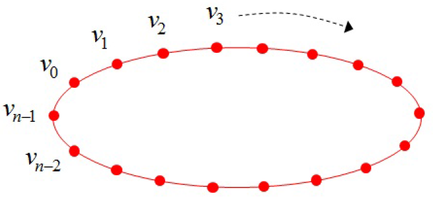
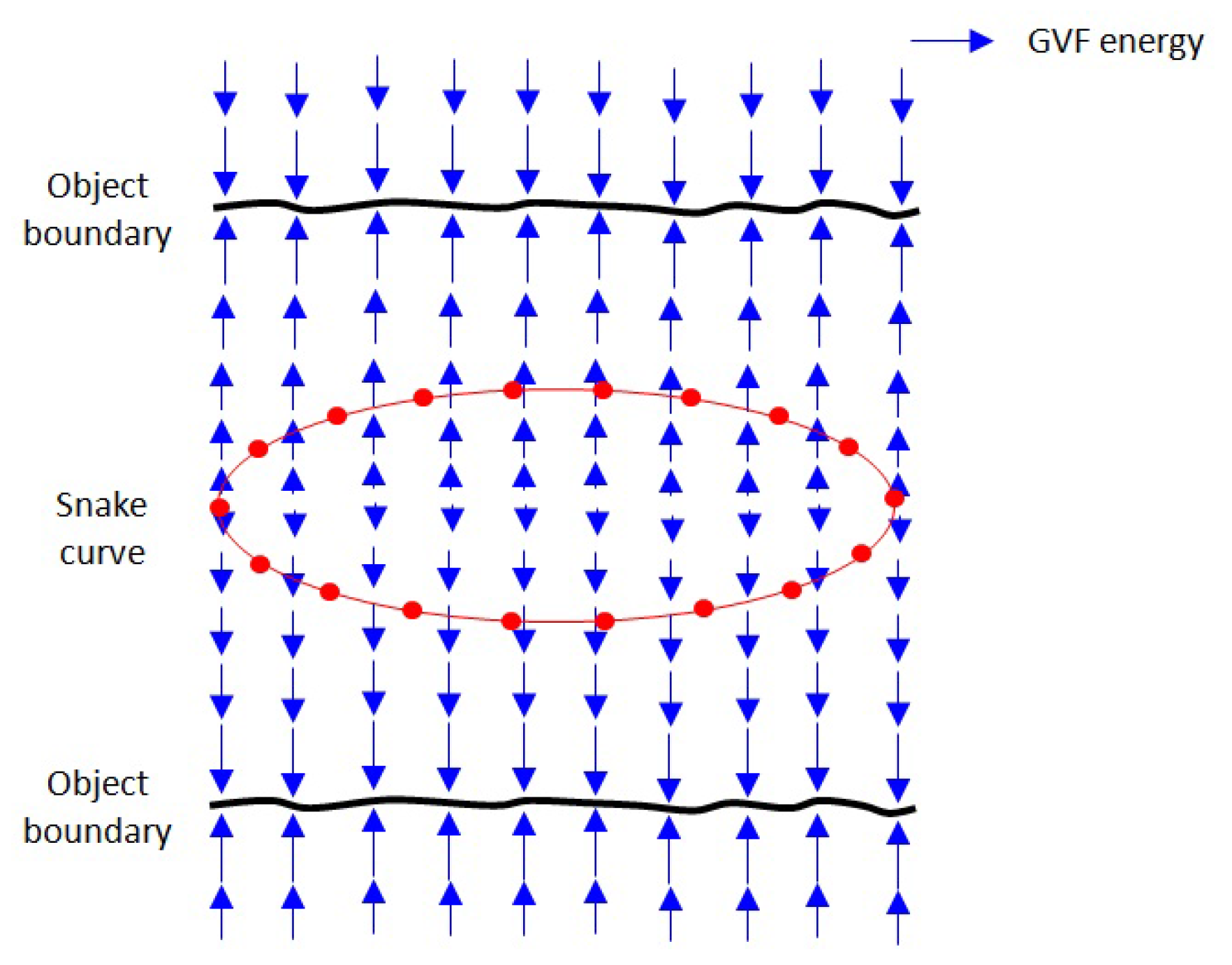
where are coordinates along the snake curve and s is the normalised arc length. The curve is represented by a set of control points and is linearly obtained by joining each control point as shown in Figure 1.
The snake’s energy function can be described as:
The energy function constituting the internal and external energy terms is described as:
where represents the internal energy term and denotes the external energy term.
The internal energy controls the snake curve’s elasticity and stiffness properties. The internal energy function can be written as:
where and are weight parameters. Equation (4) is composed of two terms, a first-order term designed to hold the curve together and a second-order term designed to keep the curve from bending. The weight parameter controls elasticity, while the weight parameter controls stiffness in the snake curve [19].
The external energy creates a gradient image that attracts the snake curve toward the object boundaries, as shown in Figure 2.
The image gradient-based external energy is described as:
where is a weighting parameter and is the gradient image of object boundaries, f.
For the snake curve to converge on the object boundary, the snake’s energy function, in Equation (3), should be minimised. To minimise the energy function, the snake curve must satisfy the Euler condition as [20]:
where is a derivative of v with respect to s. To find a solution to Equation (6), the snake is made dynamic by treating v as a function of time t, which leads to:
A solution to Equation (7) is found by discretising it and solving the discrete system iteratively [21]. When the term approaches zero, the snake’s energy function reaches its minimum and is expected to have converged on the object boundary.
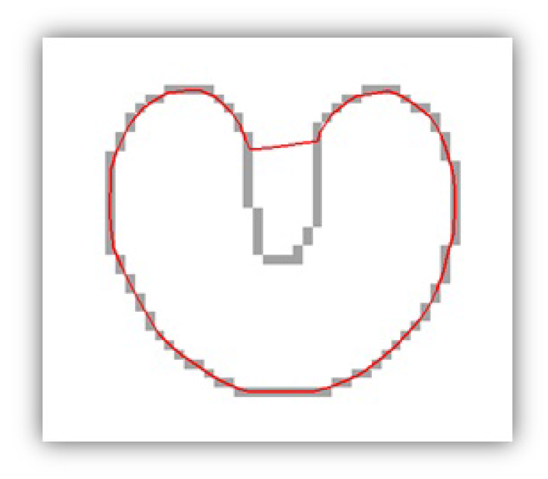
The traditional parametric active contour model has two limitations in object boundary estimation. First, the initial snake curve must be initiated close to a desirable object boundary or else it will not converge to the object boundary [22]. Second, the snake curve fails to detect concave boundaries [21], as shown in Figure 3.
Several methods have been developed to overcome these limitations in the parametric active contour model [23]. In the following sections, we discuss modified versions of the parametric active contour model that have been developed to overcome these limitations.
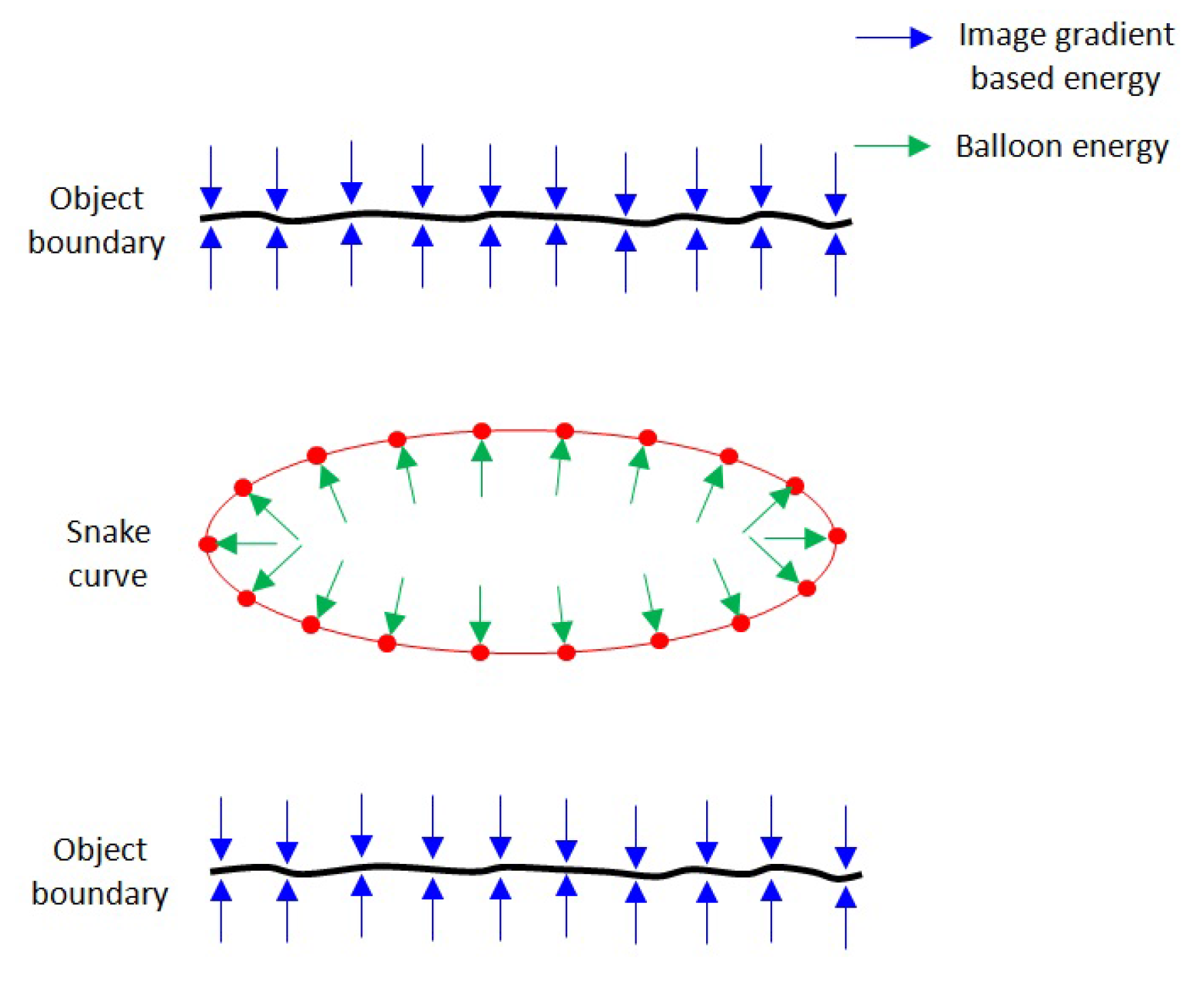
2.1.1. Balloon Model
To overcome the snake initialisation limitation, Cohen [24] introduced a balloon concept in the parametric active contour model in which an additional energy is added to the external energy term, which pushes a snake curve towards an object boundary. In the balloon model, the snake curve behaves like a balloon, which is inflated by the additional energy. The balloon energy acts in the normal direction to a point on the curve, which makes the behaviour of the snake curve more dynamic. The modified external energy term in the parametric active contour model can be described as:
where is the weight parameter for the balloon energy and is the unit vector normal to the snake curve at point . If the sign of is negative, it will have a deflating effect instead of an inflating effect over the snake curve.
The balloon energy pushes the snake curve towards object boundaries, while the image gradient-based energy attracts the snake curve toward the object boundaries, as shown in Figure 4.
If the image gradient-based energy at a point is weaker than the balloon energy, the snake curve passes beyond it. It stops at a point for which the image gradient-based energy is higher than the balloon energy. This can have the added benefit of overcoming spurious noise in the data while detecting the object boundaries [20].
The primary advantage of the balloon model is that it increases the movement range of the snake curve towards the object boundaries. It overcomes the snake curve initialisation drawback in the traditional parametric active contour model, but it does not provide a solution for the concave boundary convergence problem. The value of balloon energy is also dependent on the image gradient energy and noise in the data.
2.1.2. GVF Model
The work in [25] introduced a Gradient Vector Flow (GVF) external energy in the parametric active contour model in an attempt to detect the concave boundaries. It is based on diffused gradient vectors of the object boundaries. The GVF energy is described as the energy field , where u and v are its vector components in the plane of an image. It minimises an energy function:
Noise in the data can prohibit the GVF energy from being calculated effectively. To control the impact of this noise, a regularisation parameter, , is used to balance the first term, , and the second term, , of the Equation (9). An increased noise in the image will require a higher value for . When is small or negligible, the energy function is dominated by the first term, which is a sum of the squares of partial derivatives of the vector components. When is large, the second term dominates and minimises the energy function, when . It results in a smoothly-varying energy being produced over a homogeneous image region while not affecting the gradient energy along the object boundary.
The GVF energy is obtained by solving the following Euler equations [21]:
where is a Laplacian operator and are the gradient components along the X and Y axis of the image. Equations (10) and (11) are solved by treating u and v as functions of time t such that:
Equations (12) and (13) are known as generalised diffusion equations [21]. After estimating the value of , the external energy term, , in Equation (7), is replaced, giving us:
The GVF energy attracts the snake curve toward the object boundaries, as shown in Figure 5.
The diffused energy allows the snake curve to detect the concave boundaries [21], shown in Figure 6.
It also helps increase the movement range of the snake curve; however, its ability to overcome the snake initialisation problem is limited [26].
2.1.3. Integrated Model
We developed an integrated model in which the balloon and GVF-based parametric active contour models are combined. In the integrated model, the balloon energy pushes the snake curve, and the GVF energy attracts the snake curve toward the object boundaries, as shown in Figure 7.
This is useful in the case where there is a relatively large distance between the initial snake and the object boundaries. The use of balloon energy increases the movement range of the snake curve, while the GVF energy allows the snake curve to detect the object boundaries more efficiently. In this way, the integrated model can be applied to overcome both limitations in the traditional parametric active contour model.
2.2. Geometric Active Contour Model
The geometric active contour model is based on a level-set and curve-evolution theory [27,28]. The primary advantage of the geometric active model is that it does not require any parameters for its implementation. A geometric curve is represented implicitly as a level-set and is evolved based on geometric computations, with its speed locally dependent on the image data [20]. The level-set refers to a set of point variables for which their function is equal to some constant value. For example, the level-set of the variables can be the sphere , with centre (0,0,0) and radius r [29].
In the geometric model, the curve is represented with a zero level-set , shown in Figure 8.
The geometric curve evolves in time t on an image with a speed function,
where c is given by:
and is the potential energy derived from the input image, I. This parameter serves as the stopping term for the curve at the object boundary. The term is the gradient of the Gaussian blurred image with the standard deviation of the Gaussian distribution, . k is the curvature of the curve, which makes it smoother; is a constant, which has the effect of controlling the shrinking or expansion of the curve; and is a gradient of the level-set, . The term determines the speed with which the curve evolves along its normal direction.
The geometric curve does not stop at weak or indistinct boundary points due to its evolution speed, but continues its movement with little or no energy drawing it back [18]. To overcome this problem, an extra term can be added to Equation (15) as follows:
This additional stopping term is used to pull back the curve in case it overpasses a weak object boundary.
The advantage of using the geometric active contour model is its ability to change a curve’s topology in accordance with the shape of the object during the curve evolution process. This can be useful in object tracking and motion detection applications. The geometric active contour model is generally not useful for noisy data where the evolved curve can be accompanied by topological inconsistencies [20]. The implementation of the geometric active contour model is based on geometric computations, which results in it being a computationally-expensive process [23].
2.3. Road Extraction Using Active Contours
The concept of active contours has been extensively studied to develop several improved models, which include Generalized Gradient Vector Flow (GGVF)snake [30], region-based active contours [31], Curvature Vector Flow (CVF) snake [32], geodesic GVF/GGVF snake [33] and the Magnetostatic Active Contour (MAC) model [34]. Various active contour-based approaches have been developed for extracting roads from digital images. Youn and Bethel [35] developed an approach for extracting urban roads from aerial digital imagery using an adaptive snake. In their method, an initial approximation was provided to the snake curve by detecting the preliminary road lines based on the dominant road directions. After initialisation, an adaptive snake algorithm was applied in which the weight coefficients provided to the snake energy terms were locally modified. Yagi et al. [36] used a parametric active contour model for tracking a road and reconstructing the 3D road shape from road scenes recorded using monocular cameras. The parallel conditional of left and right sides of the road was applied as a constraint in the parametric active contour model to converge the control points to the road boundaries. Niu [37] developed a framework for semi-automatic highway extraction from high resolution aerial orthophotographs using the geometric active contour model. In their approach, the boundary and region-based information of highway features was incorporated as a constraint in the model for extraction procedure. Zhang et al. [38] used a self-adaptive template-matching method to provide the initialisation to the Least Square B-spline (LSB) snake model for extracting roads from high resolution satellite imagery. In this method, various templates of road width and the luminance attribute were matched with manually-selected points in the image, and then, the result with the maximum matching was used to initialise the snake for extracting roads.
Apart from digital images, few methods based on active contour models have been developed for extracting roads from LiDAR data. Goepfert and Rottensteiner [39] applied a snake model to extract the road network for integrating and matching, the 2D Digital Landscape Model (DLM) derived from 2D vector data and the Digital Terrain Model (DTM) generated from airborne LiDAR data. In their approach, the snake curve was initialised near the road feature using polyline vector data, while the external energy terms were derived from intensity, elevation and surface roughness-based images generated from the LiDAR data. The extracted road network information was then used to integrate the two datasets. Later, they extended their work to include building and bridge information in order to support the road extraction process using the snake model [40]. Boyko and Funkhouser [41] described a method for extracting roads from a large-scale 3D point cloud data merged from aerial and terrestrial laser scanning of an urban environment. An initial approximation of the road network in the point cloud data was made using the 2D map, and then, the road network was divided into independent patches to make the process computationally efficient. In each patch, an active contour model was applied by estimating the elevation-based attractor function as the external energy of the snake curve to find the kerbs in the urban road sections.
Active contour models present a useful approach for segmenting objects from 3D LiDAR data. One of the limiting factor associated with them is the requirement for manual intervention or a priori information for their initialisation. The development of an automated initialisation method can provide for an efficient use of active contours for the segmentation process. There is a need to develop a more robust approach for determining energy values from the input data. Several methods based on active contour models have been developed to extract road features from 2D digital images. However, their utility for segmenting 3D LiDAR point cloud has been limitedly explored. The development of a robust approach based on active contours will provide an efficient segmentation of LiDAR point cloud. LiDAR data provide elevation, intensity and pulse width information, which can be used for deriving energy terms of the active contour. In the following section, a small case study is presented in which the integrated active contour model is applied to extract road edges from MLS data.
3. Case Study
We conducted this experimental study to demonstrate the ability of active contour models in extracting road features from MLS dataset. We developed an approach in which the integrated version of parametric active contour models is applied to extract left and right edges from MLS data [42]. The implementation of the parametric active contour model is less computationally expensive in comparison with the geometric active contour model, and it gives structured control on the elasticity and stiffness properties of the snake.
In our developed approach, the input data sections are selected with some overlap between them, which allows one to batch process consecutive and overlapping road sections [43]. We use elevation and intensity attributes of the LiDAR data. These point cloud attributes are converted into 2.5D raster surfaces using point thinning and natural neighbourhood interpolation method [44]. The cell size c parameter, required to generate the raster surfaces, is selected based on an experimental analysis. The optimal value of the cell size is selected based on the performance of our approach in terms of computational cost, completeness and accuracy for its different values [43]. A slope raster surface is generated from the elevation surface. The GVF external energy terms are computed as the diffused energy field of the gradient vectors of the object boundaries from the raster surfaces. To compute the GVF energy, the object boundaries are determined from the slope and intensity raster surfaces respectively through the consecutive use of hierarchical thresholding and Canny edge detection [20]. The GVF external energy terms are estimated by iteratively diffusing gradient vector values of the object boundaries. The weight of the slope and intensity-based GVF energy terms are set with the and parameters, respectively. The balloon energy is included in the external energy by providing a weight to the normal unit vector of the snake curve points with the parameter. The values of the weight parameters for the GVF and balloon energy terms are estimated based on an experimental analysis, and then, the same values were applied for each road section. The optimal values of GVF and balloon external energy parameters are selected from their different sets of values, which can lead the snake curve to accurately converge to the road edges [45]. Internal energy is provided to the snake curve by adjusting its elasticity and stiffness properties with and weight parameters, while the step size of the snake curve is controlled with a weight parameter. The topology of the left and right edges in the road sections does not vary much; thus, the same internal energy weight parameters can be used for each road section. The optimal values of internal energy parameters are estimated from their different sets of values in an experimental analysis, the use of which with an efficient movement of the snake curve can be achieved without any jaggedness and bending [45].
The snake curve is automatically initialised over a 2.5D raster surface using the navigation track of the mobile vehicle along the road section. The snake curve moves under the influence of the internal and external energy terms. It approaches the minimum energy state during an iterative process and converges to the road edges. An example of the initial and final position of the snake curve is shown in Figure 9.
By batch processing consecutive and individual road sections, overlapping snake curves are obtained. The intersection points in between the overlapping snake curve points are found. The non-road edge points in between the intersection points of the overlapping snake curves are removed to find one continuous snake for the complete road section. Finally, the third dimension is assigned to the extracted left and right road edge points by providing the elevation from the LiDAR points nearest to them. For more information about the developed road edge extraction approach, readers can refer to [42].
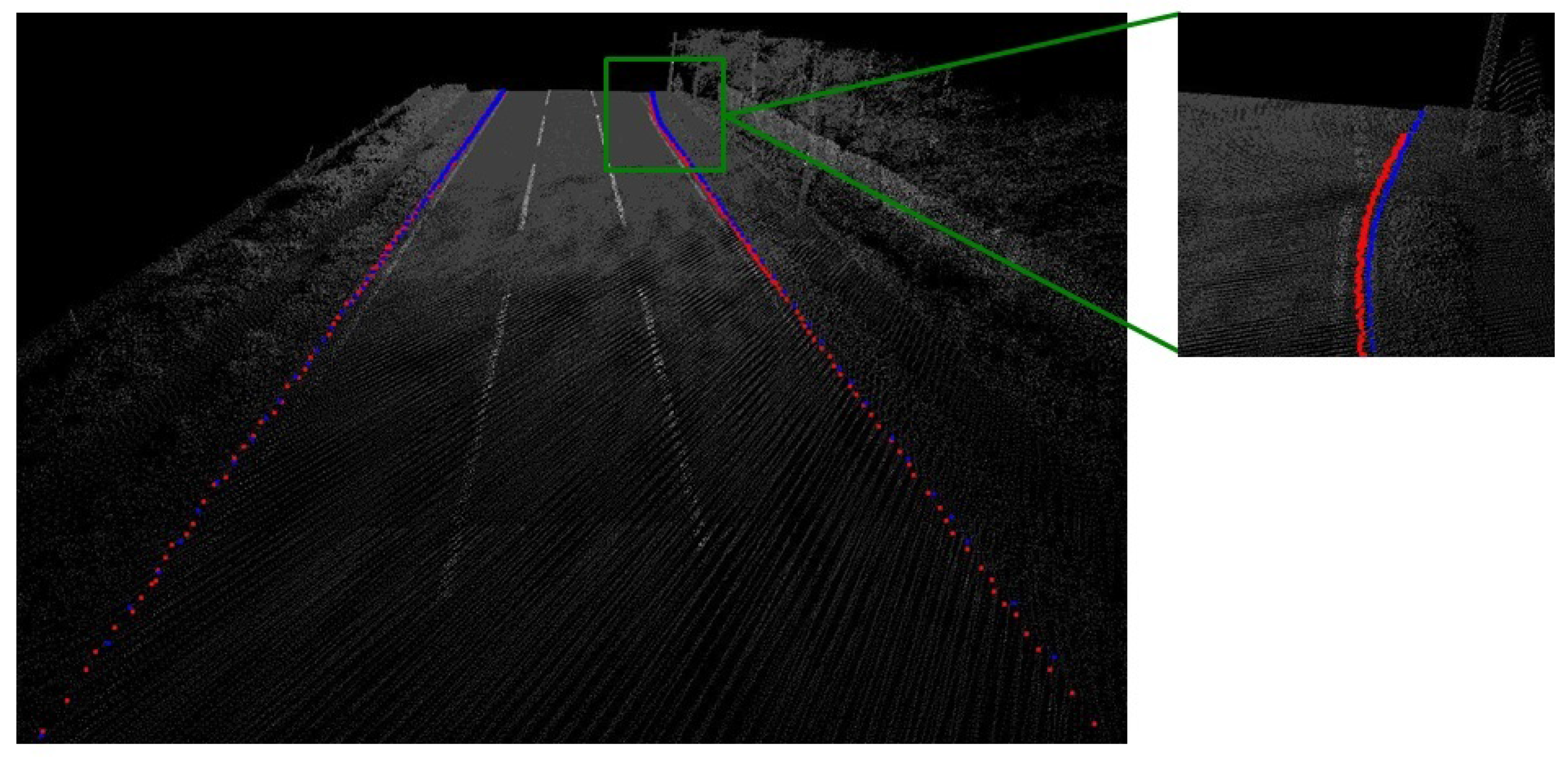
We tested our road edge extraction approach on a 50-m section of road, which consisted of a grass-soil edge along its left side and a kerb edge along its right side. This road section was selected to validate the robustness of our approach in extracting distinct sets of edges. The processed dataset for the road section were acquired using the StreetMapper MLS system in County Nottinghamshire, U.K. [46]. To process the road section, we used six sets of a 30 m × 10 m × 5 m section of LiDAR data and six sets of a 10-m section of navigation data. The road edge extraction approach was applied to the road section with parameters selected as , , , , , and . The left and right edges in the selected road section were also manually digitised in order to make a comparison with the edges extracted through our approach. The extracted 3D edges are represented in red, while the manually-digitised 3D edges are represented in blue in the road section, as shown in Figure 10.
In the next section, we validate the road edge extraction results and discuss them.
4. Results and Discussion
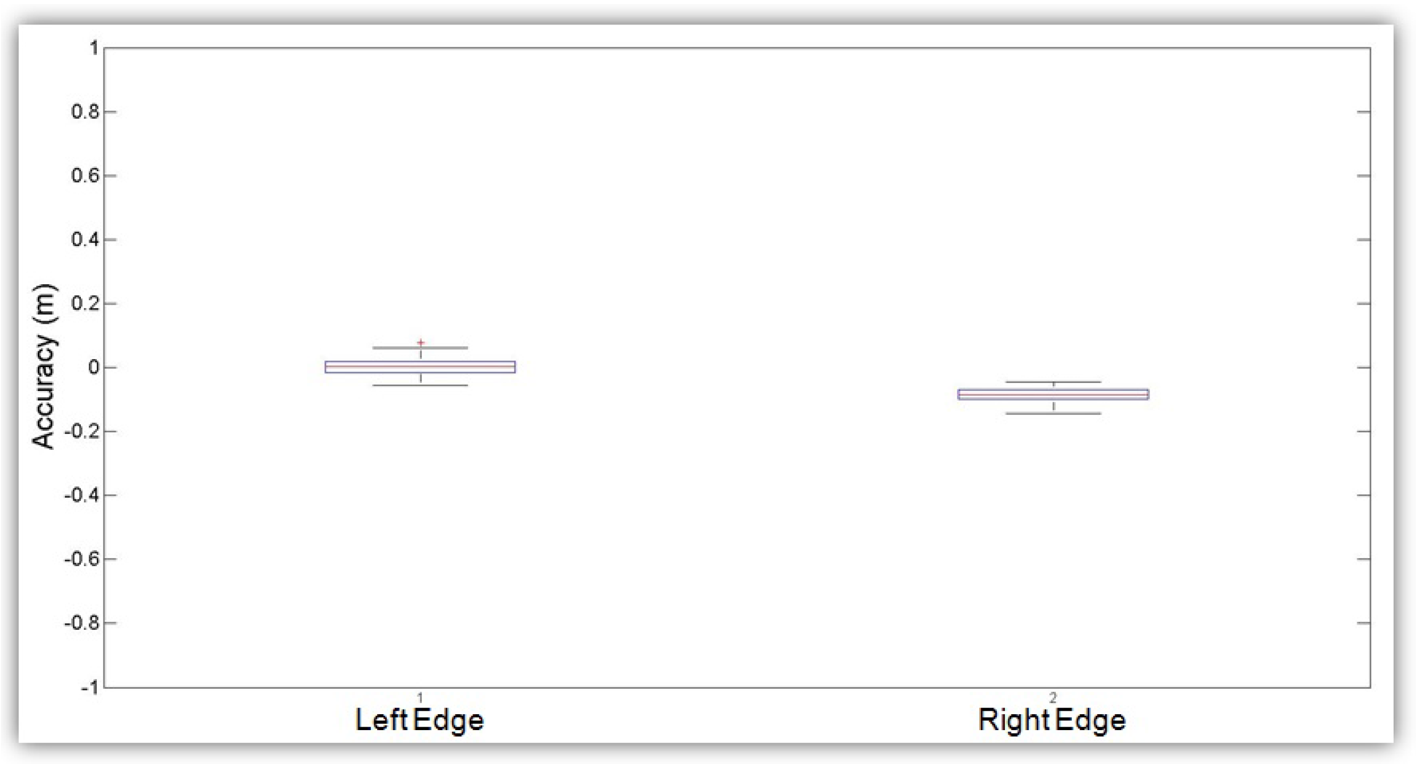
We validated the extracted 3D edges in the road section by estimating their orthogonal proximity from the manually-digitised 3D edges. These orthogonal values were estimated based on the navigation points selected at some interval along the road section [45]. The positive or negative values indicate the inside or outside position of the extracted road edge points with respect to the digitised road edge points. Box plots for the accuracy values of these extracted left and right edges in the road section are shown in Figure 11.
We also carried out statistical analyses of these accuracy values for the extracted edges as shown in Table 1.
Our approach based on the integrated parametric active contour model was able to successfully extract the left and right edges in the tested road section. The road edge extraction result displayed high accuracy values, which can also be attributed to the use of uniform and dense point cloud data along the road section. These highly dense data were acquired using a single laser scanner with a double pass approach in which the vehicle was driven back and forth on the road section. The use of such data led to the generation of smooth raster surfaces, which enabled the snake curve to precisely converge to the road edges. The minimum-maximum and lower-upper adjacent range values were lower for the right edge; however, the percentages of accuracy within -m and -m tolerances were higher for the left edge. The left edge accuracy values were found to be fully inside m, while the right edge accuracy values were fully inside m. The factors such as laser scanner position and orientation in the vehicle, scanner mirror speed, pulse repetition rate, target range and vehicle velocity may affect the point density along the left and right sides of the road section [47,48,49]. The impact of these factors on the road edge extraction results needs to be investigated.
An appropriate selection of optimal parameters is essential to extract the road edges. In this respect, we made a detailed investigation of cell size and snake energy parameters involved in our road edge extraction approach in [43,45]. The optimal value of the cell size was found by analysing the performance of the approach in raster surfaces generated with different cell sizes. In each test case of the cell size analysis, we estimated the computational cost, completeness and accuracy of the snake curve to move from its initial position to the final position. The snake curve with a 0.06 cell size required a reasonable amount of time to move, converged to the road edges to the extent with which the overlapped snake curves can be obtained and achieved an accuracy level better than in other cases. Thus, an optimal cell size of 0.06 was selected to generate the raster surfaces from the LiDAR attributes. The optimal values of internal and external energy parameters of the snake curve were estimated from their different sets of values in an experimental analyses. In our approach, the slope and intensity-based GVF energy terms were used to attract, while the balloon energy was utilised to push the snake curve toward the road edges. The use of high and weights for the GVF energy led the snake curve to move beyond the road edges, while their low values were not sufficiently strong to force it to reach the edges. We found their optimal values as four and two, respectively, which enabled the snake curve to precisely converge to the road edges. An optimal value of was found to be sufficient to push the snake curve toward road edges. In the case of internal energy parameters, the low value of the parameter caused the snake curve to be jagged at most of the points, while a high value of the parameter produced an extreme bending at some points of the snake curve. Based on this analysis, we selected their optimal values as nine and , respectively. An optimal value of parameter was chosen as three, which was sufficient to control the step size of the snake curve in order to enable it to precisely converge to the road edges. The use of these optimal values enabled the extraction of edges along the tested road section.
Guan et al. [50] reported average horizontal and vertical root mean square error (RMSE) values of m and m, respectively, for the kerb edges extracted from MLS data. In comparison, our approach extracted the kerb edges along the right side of the road section with horizontal and vertical RMSE values of m and m, respectively. The grass-soil edges along the left side of the road section were extracted with horizontal and vertical RMSE values of m, in both cases. These accuracy levels can be further improved with the use of a reflectance attribute, which is a representation of the normalised intensity values. The availability of a pulse width attribute in the acquired dataset will also allow us to use their values to generate an additional GVF energy. This will improve the road edge extraction accuracy as pulse width values can be used to distinguish the road surface from its edges more efficiently. However, the presented road edge extraction approach needs to be further tested on long road sections in order to justify its effectiveness in comparison with other existing methods.
5. Conclusions
The active contour models present a useful segmentation approach for extracting road features from LiDAR point clouds. They can be categorised as parametric and geometric active contour models based on their representation and implementation. The active contours have been extensively used to extract various features from high resolution digital images; however, they have been limitedly explored for extracting road features from LiDAR point cloud. We presented a case study in which an integrated version of parametric active contour models was applied to extract left and right edges from the MLS dataset. In the integrated version, the active contour models are combined so as to overcome the limitations existing in them. The developed road edge extraction approach is based on the assumption that the LiDAR elevation and intensity attributes can be used to distinguish the road surface from the grass-soil and the kerb edges. The successful extraction of road edges presents the potential of active contour models in extracting features from MLS data. Our novel initialisation approach based on navigation information of the mobile vehicle negated the limitation associated with the manual intervention required to initialise the active contours. Through the consecutive use of hierarchical thresholding and Canny edge detection, we made the threshold parameter estimation process more robust. The use of parametric active contour models in the developed approach facilitated making efficient utilization of specific information available about road edges in the input LiDAR data. In comparison with geometric active contours, its implementation is computationally less expensive and gives structural control over the snake for enabling it to converge to the road edges. However, the parametric active contours involve the usage of various input weight parameters, which are need to be empirically estimated. We intend to investigate the applicability of the geometric active contour model in extracting road features from LiDAR data. This could be advantageous as it will remove the requirement for weighting various input parameters. The developed approach will be tested on longer road sections with the ongoing construction of a geospatial database management system that will be able to handle 100s of kilometres of LiDAR data.
Acknowledgments
The research presented in this paper was initially funded by the Irish Research Council Enterprise Partnership scheme and the Strategic Research Cluster Grant 07/SRC/I1168 awarded by the Science Foundation Ireland under the National Development Plan. This research also received support through the Science Foundation Ireland Grant 13/IF/I2782. The research was continued at Centre Tecnològic de Telecomunicacions de Catalunya (CTTC/CERCA). The authors gratefully acknowledge this support. The authors also acknowledge the 3D Laser Mapping company for providing the StreetMapper MLS data.
Author Contributions
Pankaj Kumar collaborated with Paul Lewis in developing the approach and performing the experiments. Tim McCarthy provided technical advice at all stages. All authors contributed equally in preparing this manuscript.
Conflicts of Interest
The authors declare no conflict of interest.
Abbreviations
The following abbreviations are used in this manuscript:
| CRF | Conditional Random Field |
| CVF | Curvature Vector Flow |
| DLM | Digital Landscape Model |
| DTM | Digital Terrain Model |
| GVF | Gradient Vector Flow |
| GGVF | Generalized Gradient Vector Flow |
| LiDAR | Light Detection and Ranging |
| MAC | Magnetostatic Active Contour |
| MLS | Mobile Laser Scanning |
| NDSM | Normalized Digital Surface Model |
References
- Burtch, R. LiDAR principles and applications. In Proceedings of the Imagine Conference, Traverse City, MI, USA, 29 April–1 May 2002; pp. 1–13. [Google Scholar]
- Mallet, C.; Bretar, F. Full-waveform topographic LiDAR: State-of-the-art. ISPRS J. Photogramm. Remote Sens. 2009, 64, 1–16. [Google Scholar] [CrossRef]
- Lohani, B. Airborne Altimetry LiDAR: Principle, Data Collection, Processing and Applications. Available online: http://home.iitk.ac.in/~blohani/LiDAR_Tutorial/Airborne_AltimetricLidar_Tutorial.htm (accessed on 12 January 2016).
- Petrie, G.; Toth, C.K. Introduction to laser ranging, profiling and scanning. In Topographic Laser Ranging and Scanning: Principles and Processing; CRC Press: Boca Raton, FL, USA, 2008; pp. 1–28. [Google Scholar]
- Kumar, P.; McElhinney, C.P.; Lewis, P.; McCarthy, T. Automated road markings extraction from mobile laser scanning data. Int. J. Appl. Earth Obs. Geoinf. 2014, 32, 125–137. [Google Scholar] [CrossRef]
- Kumar, P.; Lewis, P.; McElhinney, C.P.; Abdul-Rahman, A. An algorithm for automated estimation of road roughness from mobile laser scanning data. Photogramm. Rec. 2015, 30, 30–45. [Google Scholar] [CrossRef]
- Vosselman, G. Advanced point cloud processing. In Proceedings of the Photogrammetric Week, Stuttgart, Germany, 7–11 September 2009; pp. 137–146. [Google Scholar]
- McElhinney, C.P.; Kumar, P.; Cahalane, C.; McCarthy, T. Initial results from european road safety inspection (EURSI) mobile mapping project. In Proceedings of the International Archives of Photogrammetry, Remote Sensing and Spatial Information Sciences, Newcastle, UK, 21–24 June 2010; Volume XXXVIII, pp. 440–445. [Google Scholar]
- Ibrahim, S.; Lichti, D. Curb-based street floor extraction from mobile terrestrial LiDAR point cloud. In Proceedings of the International Archives of the Photogrammetry, Remote Sensing and Spatial Information Sciences, Melbourne, Australia, 25 August–1 September 2012; Volume XXXIX, pp. 193–198. [Google Scholar]
- Zhou, L.; Vosselman, G. Mapping curbstones in airborne and mobile laser scanning data. Int. J. Appl. Earth Obs. Geoinf. 2012, 18, 293–304. [Google Scholar] [CrossRef]
- Wang, H.; Luo, H.; Wen, C.; Cheng, J.; Li, P.; Chen, Y.; Wang, C.; Li, J. Road boundaries detection based on local normal saliency from mobile laser scanning data. IEEE Geosci. Remote Sens. Lett. 2015, 12, 2085–2089. [Google Scholar] [CrossRef]
- Hui, Z.; Hu, Y.; Jin, S.; Yevenyo, Y.Z. Road centerline extraction from airborne LiDAR point cloud based on hierarchical fusion and optimization. ISPRS J. Photogramm. Remote Sens. 2016, 118, 22–36. [Google Scholar] [CrossRef]
- Xiao, L.; Wang, R.; Dai, B.; Fang, Y.; Liu, D.; Wu, T. Hybrid conditional random field based camera-LiDAR fusion for road detection. Inf. Sci. 2017. [Google Scholar] [CrossRef]
- Blake, A.; Isard, M. Active Contours, 1st ed.; Springer: London, UK, 1998. [Google Scholar]
- Kass, M.; Witkin, A.; Terzopoulos, D. Snakes: Active contour models. Int. J. Comput. Vis. 1988, 1, 321–331. [Google Scholar] [CrossRef]
- Lundervold, A.; Storvik, G. Segmentation of brain parenchyma and cerebrospinal fluid in multispectral magnetic resonance images. IEEE Trans. Med. Imaging 1995, 14, 339–349. [Google Scholar] [CrossRef] [PubMed]
- Panah, M.; Javidi, B. Segmentation of 3D holographic images using jointly distributed region snake. Opt. Express 2006, 14, 5143–5153. [Google Scholar]
- Xu, C.; Yezzi, A.; Prince, J.L. On the relationship between parametric and geometric active contours. In Proceedings of the 34th Annual Asilomar Conference on Signals, Systems and Computers, Pacific Grove, CA, USA, 30 Otober–1 November 2000; pp. 483–489. [Google Scholar]
- Kumar, P.; McCarthy, T.; McElhinney, C.P. Automated road extraction from terrestrial based mobile laser scanning system using the GVF snake model. In Proceedings of the European LiDAR Mapping Forum, Hague, The Netherlands, 30 Otober–1 December 2010; p. 10. [Google Scholar]
- Sonka, M.; Hlavac, V.; Boyle, R. Image Processing, Analysis and Machine Vision, 2nd ed.; Thomson Engineering: New York, NY, USA, 2008. [Google Scholar]
- Xu, C.; Prince, J.L. Snakes, shapes, and gradient vector flow. IEEE Trans. Image Process. 1998, 7, 359–369. [Google Scholar] [PubMed]
- Kumar, P.; McElhinney, C.P.; McCarthy, T. Utilizing terrestrial mobile laser scanning data attributes for road edge extraction using the GVF snake model. In Proceedings of the 7th International Symposium on Mobile Mapping Technology, Krakow, Poland, 13–16 June 2011; pp. 1–6. [Google Scholar]
- Kabolizade, M.; Ebadi, H.; Ahmadi, S. An improved snake model for automatic extraction of buildings from urban aerial images and LiDAR data. Comput. Environ. Urban Syst. 2010, 34, 435–441. [Google Scholar] [CrossRef]
- Cohen, L.D. On active contour models and balloons. CVGIP Image Underst. 1991, 53, 211–218. [Google Scholar] [CrossRef]
- Xu, C.; Prince, J.L. Gradient vector flow: A new external force for snakes. In Proceedings of the Computer Vision Pattern Recognition, San Juan, Puerto Rico, 17–19 June 1997; pp. 66–71. [Google Scholar]
- Kumar, P. Road Features Extraction Using Terrestrial Mobile Laser Scanning System. Ph.D. Thesis, National University of Ireland Maynooth (NUIM), Co. Kildare, Ireland, 2012. [Google Scholar]
- Caselles, V.; Catt, F.; Coll, T.; Dibos, F. A geometric model for active contours in image processing. Numer. Math. 1993, 66, 1–31. [Google Scholar] [CrossRef]
- Malladi, R.; Sethian, J.A.; Vemuri, B.C. Shape modeling with front propagation: A level set approach. IEEE Trans. Pattern Anal. Mach. Intell. 1995, 17, 158–175. [Google Scholar] [CrossRef]
- Weisstein, E.W. Level Set. Available online: http://mathworld.wolfram.com/LevelSet.html (accessed on 25 July 2012).
- Xu, C.; Prince, J. Generalized gradient vector flow external forces for active contours. Signal Process. 1998, 71, 131–139. [Google Scholar] [CrossRef]
- Chan, T.F.; Vese, L.A. Active contours without edges. IEEE Trans. Image Process. 2001, 10, 266–277. [Google Scholar] [CrossRef] [PubMed]
- Gil, D.; Radeva, P. Curvature vector flow to assure convergent deformable models for shape modelling. In Proceedings of the 4th International Workshop on Energy Minimizing Methods in Computer Vision and Pattern Recognition, Lisbon, Portugal, 7–9 July 2003; pp. 357–372. [Google Scholar]
- Paragios, N.; Gottardo, O.; Ramesh, V. Gradient vector flow fast geometric active contours. IEEE Trans. Pattern Anal. Mach. Intell. 2004, 26, 402–407. [Google Scholar] [CrossRef] [PubMed]
- Xie, X.; Mirmehdi, M. MAC: Magnetostatic active contour model. IEEE Trans. Pattern Anal. Mach. Intell. 2008, 30, 632–646. [Google Scholar] [CrossRef] [PubMed]
- Youn, J.; Bethel, J.S. Adaptive snakes for urban road extraction. In Proceedings of the International Archives of the Photogrammetry, Remote Sensing and Spatial Information Sciences, Istanbul, Turkey, 12–23 July 2004; Volume 35, pp. 465–470. [Google Scholar]
- Yagi, Y.; Brady, M.; Kawasaki, Y.; Yachida, M. Active contour road model for road tracking and 3D road shape reconstruction. Electron. Commun. Jpn. Part 3 2005, 88, 1597–1607. [Google Scholar] [CrossRef]
- Niu, X. A geometric active contour model for highway extraction. In Proceedings of the ASPRS Annual Conference, Reno, NV, USA, 1–5 May 2006. [Google Scholar]
- Zhang, H.; Xiao, Z.; Zhou, Q. Research on road extraction semi-automatically from high resolution remote sensing images. In Proceedings of the International Archives of the Photogrammetry, Remote Sensing and Spatial Information Sciences, Beijing, China, 3–11 July 2008; Volume 37, pp. 535–538. [Google Scholar]
- Goepfert, J.; Rottensteiner, F. Adaption of roads to ALS data by means of network snakes. In Proceedings of the International Archives of the Photogrammetry, Remote Sensing and Spatial Information Sciences, Paris, France, 1–2 September 2009; Volume 38, pp. 24–29. [Google Scholar]
- Goepfert, J.; Rottensteiner, F. Using building and bridge information for adapting roads to ALS data by means of network snakes. In Proceedings of the International Archives of the Photogrammetry, Remote Sensing and Spatial Information Sciences, Paris, France, 1–3 September 2010; Volume XXXVIII, pp. 163–168. [Google Scholar]
- Boyko, A.; Funkhouser, T. Extracting roads from dense point clouds in large scale urban environment. ISPRS J. Photogramm. Remote Sens. 2011, 66, S2–S12. [Google Scholar] [CrossRef]
- Kumar, P.; McElhinney, C.P.; Lewis, P.; McCarthy, T. An automated algorithm for extracting road edges from terrestrial mobile LiDAR data. ISPRS J. Photogramm. Remote Sens. 2013, 85, 44–55. [Google Scholar] [CrossRef]
- Kumar, P.; Lewis, P.; McElhinney, C.P. Parametric analysis for automated extraction of road edges from mobile laser scanning data. In Proceedings of the ISPRS Annals of the Photogrammetry, Remote Sensing and Spatial Information Sciences, KualaLumpur, Malaysia, 28–30 October 2015; pp. 215–221. [Google Scholar]
- Crawford, C. Minimising Noise from LiDAR for Contouring and Slope Analysis. 2009. Available online: http://blogs.esri.com/esri/arcgis/2009/09/02 (accessed on 7 June 2012).
- Kumar, P.; Lewis, P.; McElhinney, C.P.; Boguslawski, P.; McCarthy, T. Snake energy analysis and result validation for a mobile laser scanning data based automated road edge extraction algorithm. IEEE J. Sel. Top. Appl. Earth Obs. Remote Sens. 2017, 10, 763–773. [Google Scholar] [CrossRef]
- StreetMapper. 3D Laser Mapping. 2005. Available online: http://www.3dlasermapping.com/streetmapper (accessed on 15 December 2016).
- Cahalane, C.; McElhinney, C.P.; Lewis, P.; McCarthy, T. MIMIC: An innovative methodology for determining mobile laser scanning system point density. Remote Sens. 2014, 6, 7857–7877. [Google Scholar]
- Cahalane, C.; Lewis, P.; McElhinney, C.P.; McCarthy, T. Optimising mobile mapping system laser orientation. ISPRS Int. J. Geo-Inf. 2015, 4, 302–319. [Google Scholar] [CrossRef]
- Cahalane, C.; Lewis, P.; McElhinney, C.P.; McNerney, E.; McCarthy, T. Improving MMS Performance during Infrastructure Surveys through Geometry Aided Design. Infrastructures 2016, 1, 5. [Google Scholar] [CrossRef]
- Guan, H.; Li, J.; Yu, Y.; Chapman, M.; Wang, C. Automated road information extraction from mobile laser scanning data. IEEE Trans. Intell. Transp. Syst. 2015, 16, 194–205. [Google Scholar] [CrossRef]
Figure 1.
Snake curve initialised in the form of a parametric ellipse.

Figure 2.
Snake curve initialised on the gradient image of object boundaries.
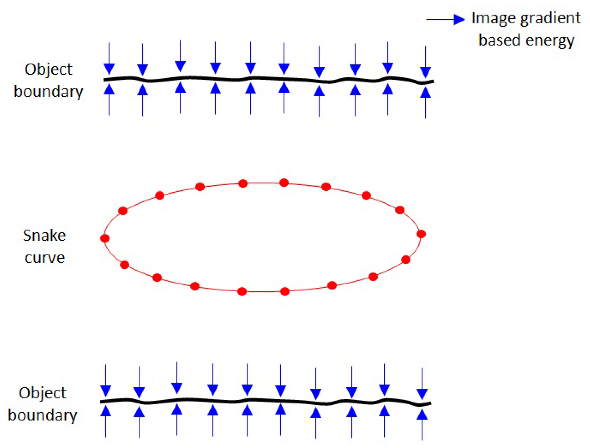
Figure 3.
Parametric active contour model applied to an object with a concave boundary [21].
Figure 3.
Parametric active contour model applied to an object with a concave boundary [21].

Figure 4.
Balloon external energy added to the snake curve.

Figure 5.
Snake curve initialised on the GVF image of object boundaries.

Figure 6.
GVF-based parametric active contour model applied to an object with a concave boundary [21].
Figure 6.
GVF-based parametric active contour model applied to an object with a concave boundary [21].
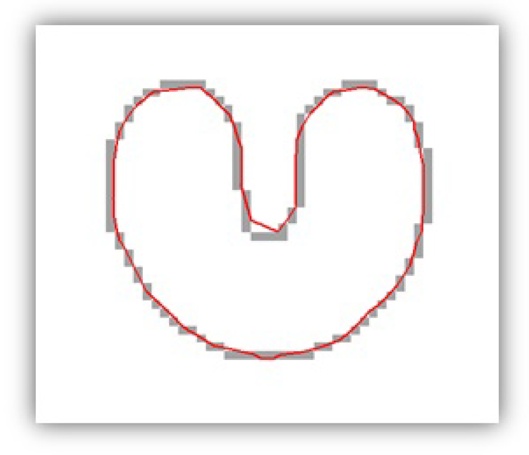
Figure 7.
Balloon energy pushes the snake curve, and GVF energy attracts the snake curve toward the object boundaries.
Figure 7.
Balloon energy pushes the snake curve, and GVF energy attracts the snake curve toward the object boundaries.
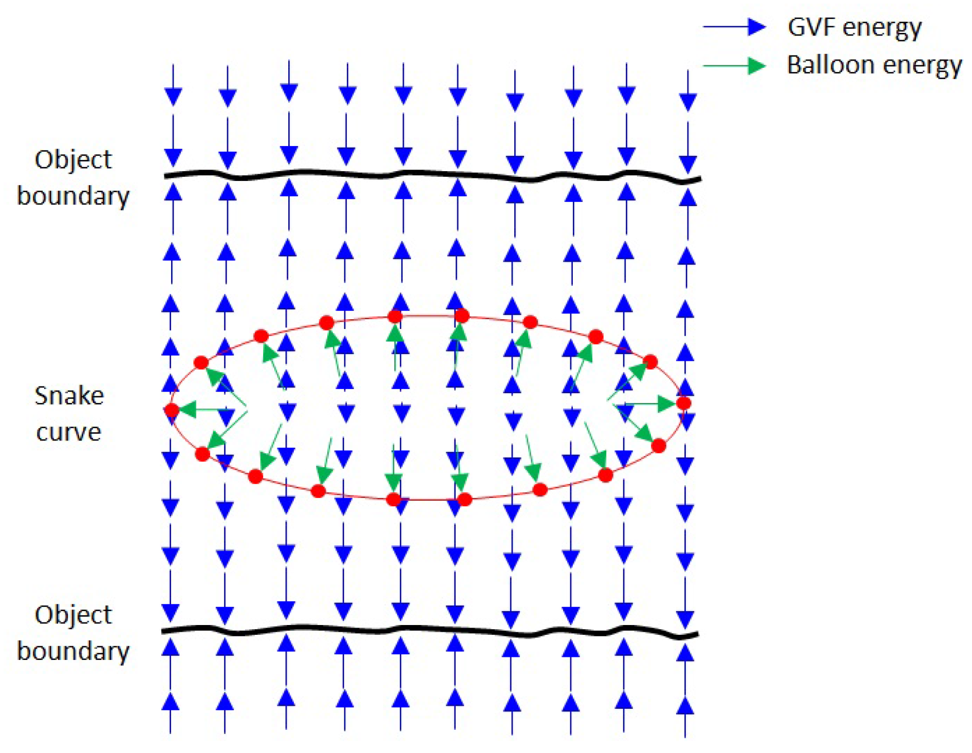
Figure 8.
Geometric active contour model.
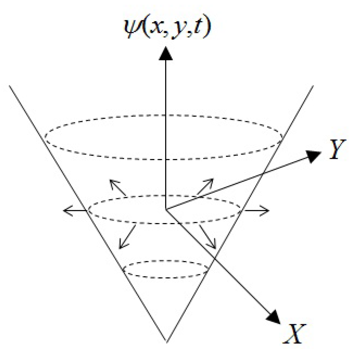
Figure 9.
An (a) initial and (b) final position of the snake curve.
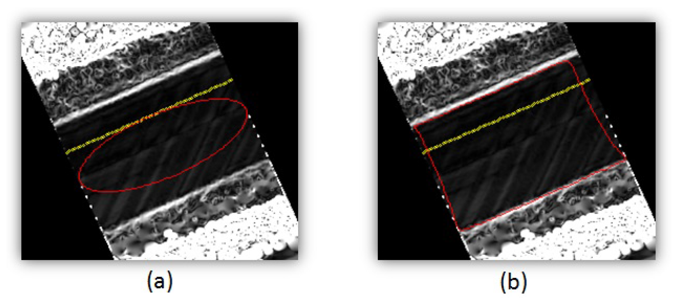
Figure 10.
The extracted 3D edges are represented in red, and the manually-digitised 3D edges are represented in blue in the 50-m road section. The inset picture of right edge shows some of the points in detail.
Figure 10.
The extracted 3D edges are represented in red, and the manually-digitised 3D edges are represented in blue in the 50-m road section. The inset picture of right edge shows some of the points in detail.

Figure 11.
Box plot for the accuracy values of the extracted left and right edges in the road section.
Figure 11.
Box plot for the accuracy values of the extracted left and right edges in the road section.


Table 1.
Statistical analysis of the accuracy values of the extracted left and right edges in the road section.
Table 1.
Statistical analysis of the accuracy values of the extracted left and right edges in the road section.
| Left Edge | Right Edge | |
|---|---|---|
| minimum (m) | −0.055 | −0.145 |
| maximum (m) | 0.078 | −0.046 |
| lower adjacent (m) | −0.055 | −0.145 |
| upper adjacent (m) | 0.061 | −0.046 |
| 25th percentile (m) | −0.016 | −0.099 |
| 75th percentile (m) | 0.019 | −0.068 |
| mean (m) | 0.001 | −0.088 |
| median (m) | 0.001 | −0.086 |
| outliers (%) | 1.64 | 0 |
| inside (%) | 26.26 | 0 |
| inside (%) | 100 | 75.41 |
| inside (%) | 100 | 100 |
| horizontal RMSE (m) | 0.02 | 0.09 |
| vertical RMSE (m) | 0.02 | 0.02 |
© 2017 by the authors. Licensee MDPI, Basel, Switzerland. This article is an open access article distributed under the terms and conditions of the Creative Commons Attribution (CC BY) license (http://creativecommons.org/licenses/by/4.0/).
Share and Cite
MDPI and ACS Style
Kumar, P.; Lewis, P.; McCarthy, T. The Potential of Active Contour Models in Extracting Road Edges from Mobile Laser Scanning Data. Infrastructures 2017, 2, 9. https://doi.org/10.3390/infrastructures2030009
AMA Style
Kumar P, Lewis P, McCarthy T. The Potential of Active Contour Models in Extracting Road Edges from Mobile Laser Scanning Data. Infrastructures. 2017; 2(3):9. https://doi.org/10.3390/infrastructures2030009
Chicago/Turabian StyleKumar, Pankaj, Paul Lewis, and Tim McCarthy. 2017. "The Potential of Active Contour Models in Extracting Road Edges from Mobile Laser Scanning Data" Infrastructures 2, no. 3: 9. https://doi.org/10.3390/infrastructures2030009