Dynamic Amplification Factor of Continuous versus Simply Supported Bridges Due to the Action of a Moving Vehicle


Civil Engineering School, University College Dublin, Dublin 4, Ireland
*
Author to whom correspondence should be addressed.
Infrastructures 2018, 3(2), 12; https://doi.org/10.3390/infrastructures3020012
Submission received: 19 April 2018
/
Revised: 17 May 2018
/
Accepted: 17 May 2018
/
Published: 18 May 2018
(This article belongs to the Special Issue Feature Papers)
Abstract
:Research to date on Dynamic Amplification Factors (DAFs) caused by traffic loading, mostly focused on simply supported bridges, is extended here to multiple-span continuous bridges. Emphasis is placed upon assessing the DAF of hogging bending moments, which has not been sufficiently addressed in the literature. Vehicle-bridge interaction simulations are employed to analyze the response of a finite element discretized beam subjected to the crossing of two vehicle types: a 2-axle-truck and a 5-axle truck-trailer. Road irregularities are randomly generated for two ISO roughness classes. Noticeable differences appear between DAF of mid-span moment in a simply supported beam, and DAFs of the mid-span sagging moment and of the hogging moment over the internal support in a continuous multiple-span beam. Although the critical location of the maximum static moment over the internal support may indicate that DAF of hogging moment would have to be relatively small, this paper provides evidence that this is not always the case, and that DAFs of hogging moments can be as significant as DAF of sagging moments.
1. Introduction
The dynamic behavior of beam structures (i.e., bridges where one dimension is significantly larger than the other two) on highways and railways subjected to moving loads has been investigated for over a century [1]. The last four decades have seen several authors investigating and explaining the reasons behind the dynamic impact caused by moving vehicles on the bridge response. “Dynamic increment” [2], “impact factor” or “dynamic load allowance” [3], “dynamic increment factor” [4], “dynamic load allowance” [5] and “dynamic amplification factor” or “DAF” [6,7,8] are some of the terms employed in quantifying the dynamic impact with respect to the static response. Bending moment is the load effect investigated in this paper, where DAF is calculated dividing the maximum total bending moment (“static” + “dynamic”) by the maximum static bending moment for a given section “A-A” due to the crossing of a vehicle (Equation (1)). If only the static response of a simply supported bridge was considered, bending moments due to a moving vehicle tend to be largest at mid-span. For this reason, the “A-A” section used as a reference is generally the mid-span section [7].
DAF due to traffic has been assessed mostly for simply supported bridges and there is not an equivalent amount of research for continuously supported bridges. For instance, the comprehensive reviews on the topic by [9,10] do not distinguish between DAF in simply supported and in continuous bridges. This is justified not only by the significant proportion of single-span structures among the bridge stock, but also by those multi-span structures constructed as a series of simply supported spans. However, the continuous solution is becoming increasingly popular. From a structural point of view, the use of continuous deck reduces the bridge deck thickness compared to a simply supported solution. From a construction and maintenance point of view, the reduction in the number of joints in continuous bridges also represents substantial cost savings [11]. Additionally, the influence of factors such as rail irregularity, ballast stiffness, suspension stiffness and suspension damping appears to be smaller for continuous bridges than simply supported bridges. These factors can affect drastically the riding comfort of the train cars traveling over bridges [12]. In a recent publication, ref. [13] report on DAF results for sagging bending moment in continuous bridges; however, there is no mention to hogging moments. The modes of vibration of a structure are characterized by their mode shape and their modal frequency. For a given mode of vibration, there are points of the mode shape that are always zero, which are referred to as nodes. The location of the maximum static hogging moment, i.e., over the internal support, corresponds to a node for all modes of vibration of a continuous bridge. The fact that there is no modal contribution at a node (i.e., the displacement remains zero at all times) may lead to the belief that the hogging moment will experience only small dynamic increments with respect to its static value (i.e., purely due to the varying vehicle dynamic forces). While this may be true for the section located exactly over the internal supports in the case of low dynamic vehicle forces, the same cannot be said for high dynamic vehicular forces (i.e., as a result of very rough profiles) or nearby sections where static hogging moment could still be significant and combined with dynamic contributions not only from the vehicle but also from the bridge inertial forces.
Full Dynamic Amplification Factor (FDAF) is another term used to quantify the relative dynamic increment that addresses maximum total response and maximum static response may not necessarily occur at the same location. It is introduced first by [14], who define FDAF as the ratio of the maximum total load effect across the bridge length to the highest static load effect at a particular section taken as reference (i.e., mid-span). They report on FDAFs for simply supported beams, but these calculations are not available for continuous beams yet.
This paper seeks to fill gaps in the DAF literature by determining the dynamic impact for the maximum moments on a continuous beam model with two equal spans. DAFs are obtained for sagging moments in both the 1st and 2nd span as well as hogging moments over the internal support. DAFs and FDAFs of a continuous bridge are compared to a simply supported bridge. The authors build on preliminary work that analyses DAF of multi-span continuous beams when traversed by vehicle models consisting of moving constant point loads [15]. This paper discusses key parameters on the dynamic response of a bridge such as variations in vehicle dynamics, vehicle configuration, road profile and the interaction between the bridge and the vehicle.
2. Finite Element Modelling of Vehicle-Bridge Interaction
A review of Vehicle-Bridge Interaction (VBI) algorithms available in the literature can be found in [16]. This paper employs a coupled Finite Element (FE) VBI algorithm, similar to that used by [17] and [18], which has been experimentally tested using measurements of the response of a scaled bridge to the crossing of a scaled 2-axle vehicle over a rough surface in [19]. The structural response is calculated by solving the equations of motions of the combined vehicle-bridge system for each time step. Unlike the uncoupled approach, the system matrices vary with the position of the vehicle on the bridge and there is no need for iterations to ensure compatibility between bridge and vehicle models at each time step. The vehicle and bridge models and the coupled VBI procedure employed in this paper are set out in the following sub-sections.
2.1. Vehicle Model
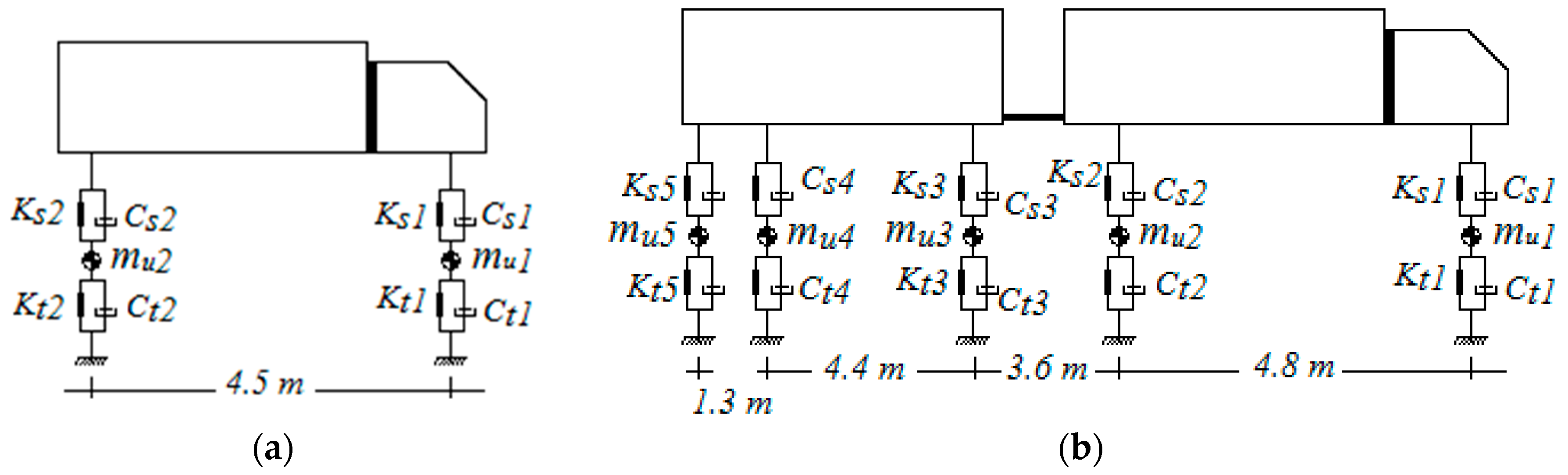
The responses of the beam models are obtained for planar 2-axle and 5-axle trucks to assess the influence of multiple axles and vehicle length on the DAF-velocity pattern. Figure 1 gives the configurations adopted for these two vehicle types based on the European Committee for Standardization [20]. The static weights of the 2-axle vehicle are 90 kN and 190 kN for the front and rear axles respectively, while those of the 5-axle vehicle are 90 kN, 180 kN, 120 kN, 110 kN and 110 kN for the first to the fifth axle [20].
Table 1 and Table 2 provide the mechanical properties of the two vehicle models, taking as reference values suggested by [21] and [22]. The characteristics of these numerical models are as follows:
- The 2-axle model represents a rigid truck with four Degrees of Freedom (DOFs) corresponding to axle hop displacements (yu1, yu2) of the two axle masses (un-sprung masses, mu1 and mu2), bounce displacement, ys1, as well as the pitch rotation, θT1, of the body mass (sprung mass, ms). The two axle masses are linked to the road surface by means of linear springs of stiffness (Kt1 and Kt2) and damping elements (Ct1 and Ct2) representing the tires. The body mass is linked to the two axle masses with the help of springs of stiffness Ks1 and Ks2 that have linear viscous dampers, with values of Cs1 and Cs2 respectively, representing the suspensions.
- The 5-axle model is a truck comprising two major bodies, truck and trailer, with a total of 9 DOFs. Four of these DOFs are located in the tractor and they correspond to axle hop displacements (yu1, and yu2) of the two axle masses (un-sprung masses, mu1 and mu2), bounce displacement, ys1, as well as the pitch rotation, θT1, of the body mass (sprung mass, ms1). The two axle masses are linked to the road surface by means of linear springs of stiffness (Kt1 and Kt2) and damping elements (Ct1 and Ct2) representing the tires. The body mass is linked to the axle masses with the help of springs of stiffness Ks1 and Ks2 that have linear viscous dampers, with values of Cs1 and Cs2 respectively, representing the suspensions. Another 5 DOFs are located in the trailer, and they correspond to the axle hop displacements (yui (i = 3 to 5) of each axle mass (un-sprung masses mui with i = 3 to 5)), bounce displacement, ys2, and pitch rotation, θT2, of body mass (sprung mass, ms2). The same description of the tire and suspensions elements of the tractor apply to the trailer. Tire elements are labelled Kti (i = 3 to 5) and Cti (i = 3 to 5), and suspension elements Ksi (i = 3 to 5) and Csi (i = 3 to 5).
The equations of motion of the vehicles’ models are obtained by imposing equilibrium of all forces and moments acting on the masses and expressing them in terms of the degrees of freedom:
where [Mv], [Cv] and [Kv] are mass, damping and stiffness matrices of the vehicle, respectively and , and are the respective vectors of nodal acceleration, velocity and displacement. is the time-varying dynamic interaction force vector applied to the vehicle’s DOFs.
2.2. Bridge Model
The simply supported beam model has a total length of 15 m, while the continuous two-span beam model has 30 m (each span is 15 m). The beam models are discretized using the FE method. The length of each element is 0.5 m, therefore, the simply supported and continuous models are made of thirty and sixty discretised beam elements respectively with four DOFs per beam element (2 per node). The vertical displacements at the end nodes over the support sections are restrained. Bridge properties, based on [23], are constant mass per unit length, , of 28,125 m−1 kg, modulus of elasticity, E, of 35 GPa, and second moment of area, I, of 0.5273 m4. The first natural frequency of the continuous and simply supported bridge models is 5.65 Hz.
The response of the beam model to a series of time-varying forces is given by the system of equations:
where [Mb], [Cb] and [Kb] are the respective mass, damping and stiffness matrices of the beam model and , and are vectors of nodal bridge acceleration, velocity and displacement, respectively. Rayleigh damping is used here, which is given by:
where and β are constants. These constants are obtained from and , where and are the first two circular natural frequencies of the bridge. The damping ratio ζ is assumed to be 0.03 and the same for all modes [24].
2.3. Road Profile
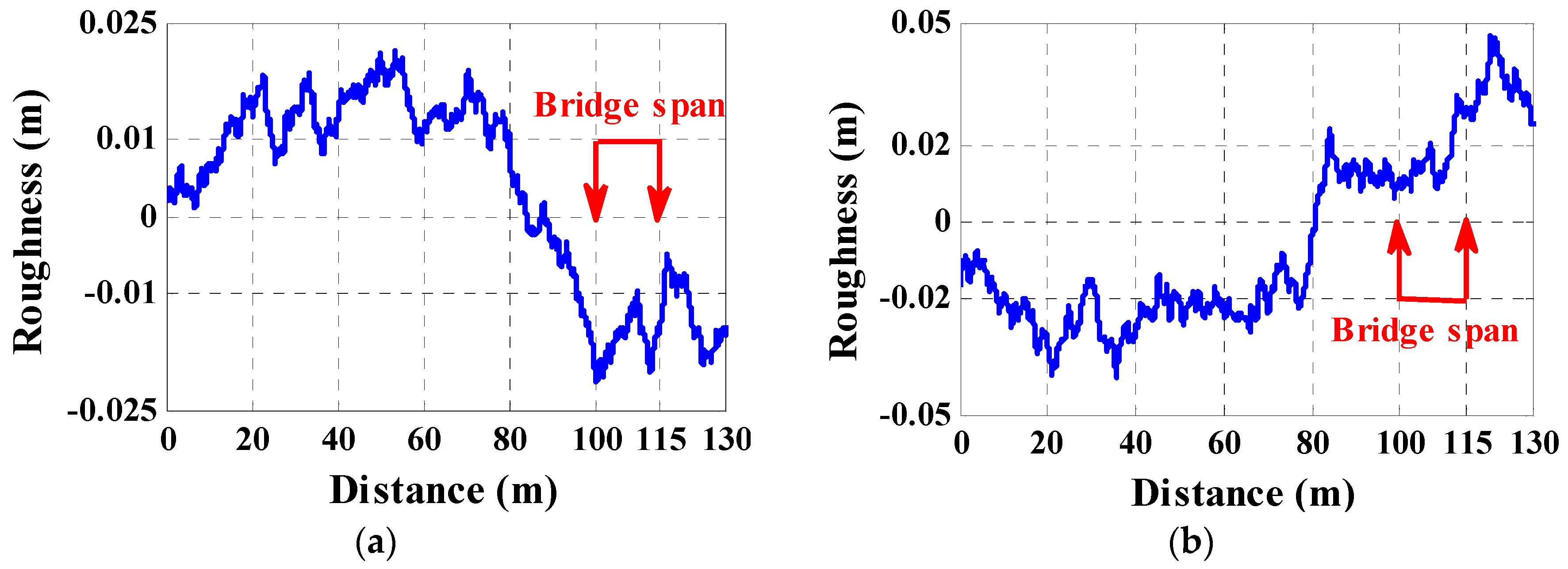
The roughness of the road surface is acknowledged to be the main cause for dynamic excitation in vehicle-induced bridge vibrations [25,26,27]. According to International Organization for Standardization [28], an artificial road profile can be generated stochastically using the Power Spectral Density function of vertical displacements along with the inverse fast Fourier transform technique explained by [29]. Here, the total number of spatial waves used to construct the road profile is 1000. A random phase angle is sampled for each spatial wave from a uniform probabilistic distribution in the range of 0-2. In this paper, 100 road profiles are randomly generated for road classes “A” (i.e., very good) and “B” (i.e., good) [28]. In these random profiles, the respective mean value and the standard deviation employed for the geometric spatial mean are m3/cycle and for class “A” and m3/cycle and for class “B” [30]. A moving average filter is applied to the generated road profile heights over a distance of 0.24 m to simulate the attenuation of short wavelength disturbances by the tire contact patch [25,31]. Furthermore, a road approach that spans over 100 m is added before the bridge to induce initial conditions of dynamic equilibrium in the vehicle. Figure 2 shows an instance of class “A” and of class “B” road profiles of 130 m length, including the 100 m approach.
2.4. Coupling of the VBI system
The dynamic interaction between the vehicle and the bridge is implemented in MATLAB [32]. The vehicle and the bridge are coupled at the tire contact points via the interaction force vector . Combining Equations (2) and (3), the coupled equation of motion is formed as:
where [Mg] is the combined system mass matrix, and [Cg] and [Kg] are the coupled time-varying system damping and stiffness matrices, respectively. The vector is the displacement vector of the system. is the coupled force vector system. In this paper, the coupled force vector has different formulae depending on the vehicle system; whether a truck (Equation (6)) or a truck-trailer (Equation (7)) is employed:
where:
- the zero elements in the force vectors correspond to pitching and heaving DOFs for the trucks and trailers.
- is an (n × nf) matrix which distributes the nf applied interaction forces on beam elements to equivalent forces acting on the nodes (i.e., nf is equal to 2 and 5 for the 2- and 5-axle vehicles respectively) and n is the total number of DOFs of the beam (i.e., n is equal to 60 and 120 for the single span and two-span beam FE models respectively).
- Pi is the static axle weight corresponding to axle i of the vehicle.
- ri is the road profile displacement under axle i.
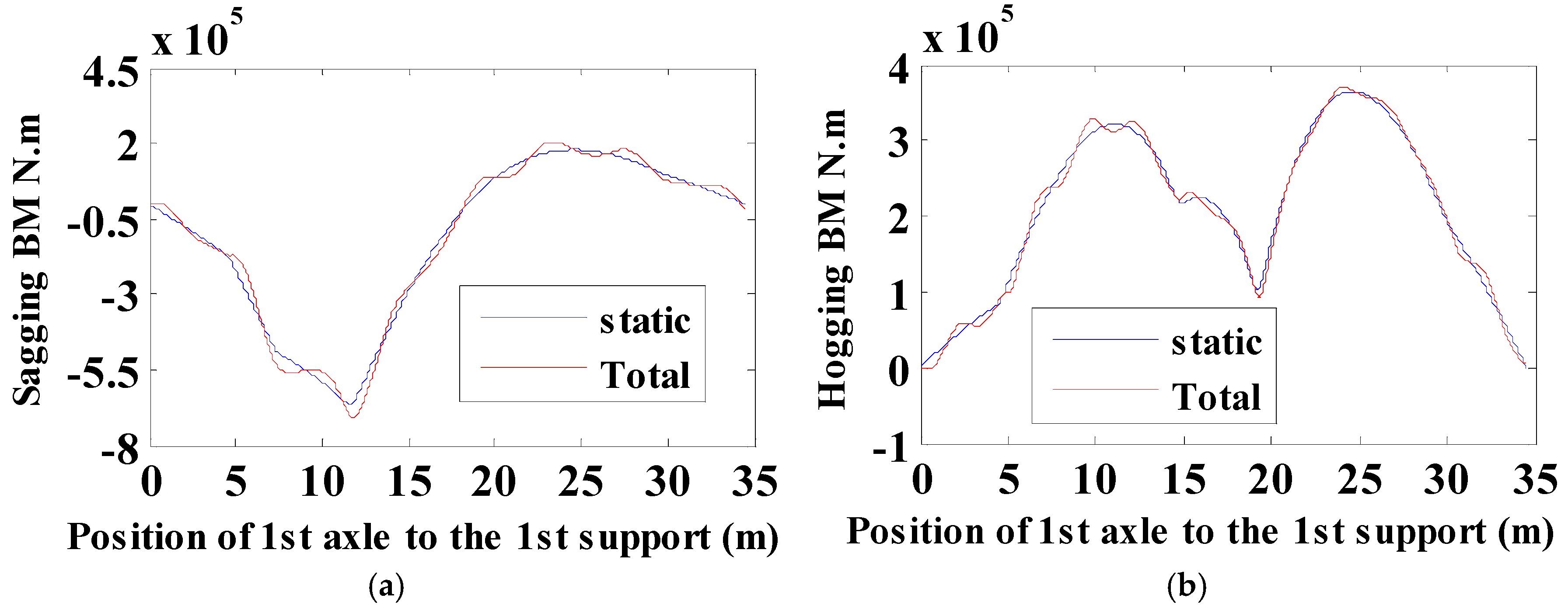
The equations for the coupled system are solved using the Wilson-Theta integration scheme [33] with a time interval of 0.002 s. The optimal value of the parameter = 1.420815 is used for unconditional stability in the integration scheme. The initial conditions are considered to be zero displacements, velocities and accelerations in all solutions. The static bridge response is calculated by driving the static weights of the vehicles at a quasi-static velocity (0.3 m/s) over a smooth road profile. The static component of sagging moment and the total sagging moment at mid-length of the 1st span of the two-span model due to a 2-axle truck (two-constant point loads) travelling at 25 m/s are illustrated in Figure 3a. Figure 3b represents the hogging moment over the internal support for the same loading scenario.
3. Dynamic Amplification Factors
DAFs and FDAFs of simply supported and continuous bridge models are calculated for comparison purposes. Calculations are carried out for vehicle velocities from 10 km/h to 120 km/h in increments of 1.08 km/h.
3.1. Simply Supported Beam
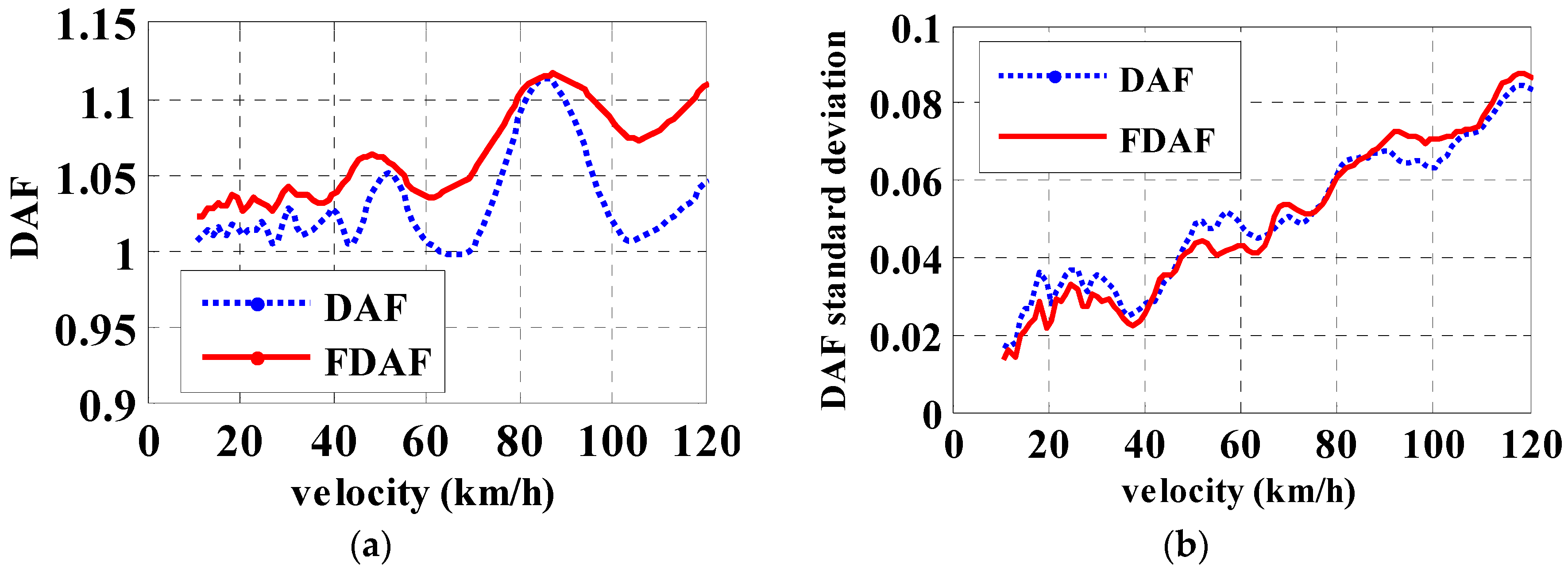
Figure 4a,b shows the mean and standard deviation respectively of DAF values due to the 2-axle truck travelling on 100 class “B” road profiles. It is noted that the highest mean value of DAF is equal to 1.12 and identical to the highest FDAF for a velocity of 85.32 km/h. Standard deviations of DAF and FDAF are found to be 0.065 for this critical velocity.
Figure 5a,b shows the mean and standard deviation respectively, of DAF/FDAF, due to the 5-axle truck travelling on 100 profiles of road class “B”. The highest mean value of FDAF is 1.173 with a standard deviation of 0.07 for a velocity of 92.88 km/h. Meanwhile, the highest mean value of DAF is 1.144 with a standard deviation of 0.064 for a velocity of 91.8 km/h.
Similar trends in mean (µ) and standard deviation (σ) are observed for road classes “A” and “B”. Table 3 summarizes the highest mean DAF and FDAF values and the critical velocities at which they occur. The standard deviation of maximum DAF and FDAFs for class “B” are always higher than for class “A” due to the larger uncertainty associated with the rougher profile. However, maximum mean DAF and FDAF and critical velocity due to the 2-axle vehicle are equal for both road classes. It appears that the dynamic forces of the 2-axle vehicle do not reach sufficiently high values with class “B” as to distort the trend found with class “A”, which is mostly determined by the bridge inertial forces as well as vehicle configuration and velocity. The effect of road roughness is felt more strongly by the 5-axle vehicle, where differences between mean DAF and FDAFs of both road classes are noticeable.
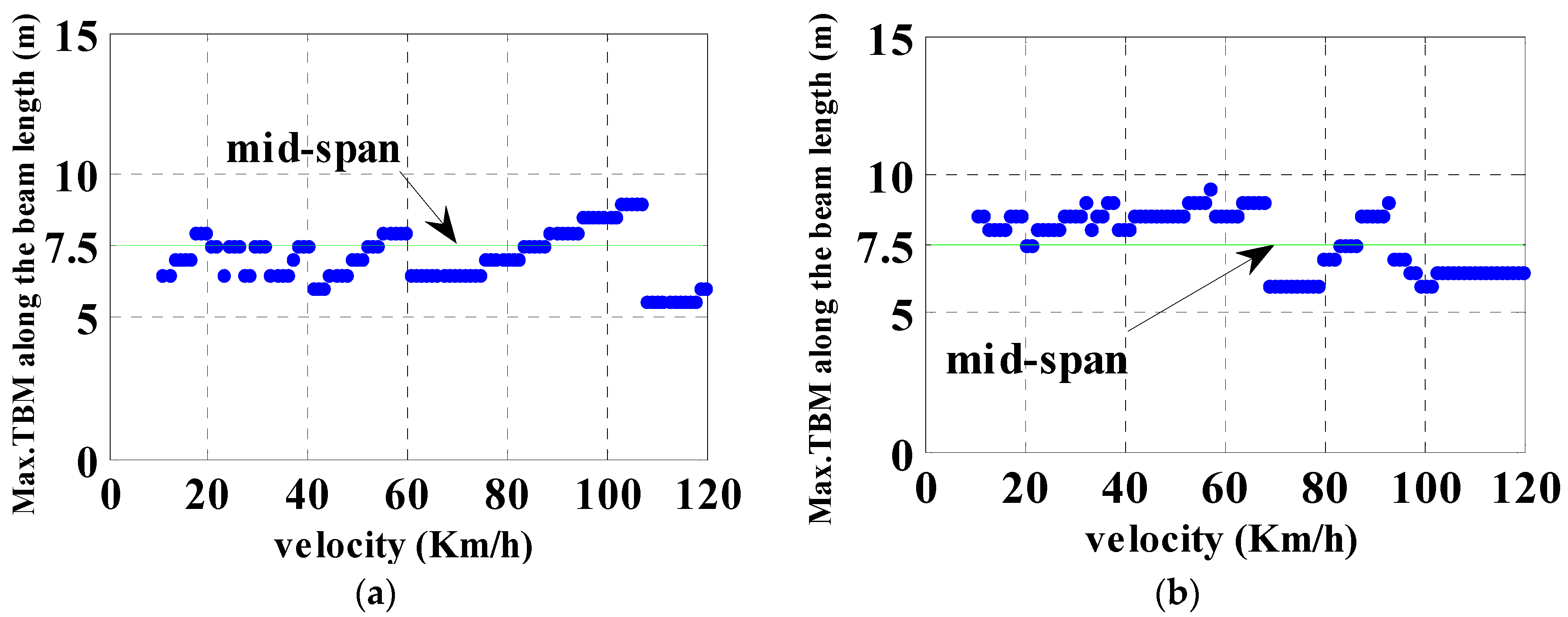
By definition, FDAF is always equal to or larger than DAF, as any differences are due to the maximum total bending moment (TBM) developing in a location different from mid-span. The locations where the maximum total bending moment takes place are illustrated in Figure 6 for each vehicle velocity.
3.2. Continuous Beam
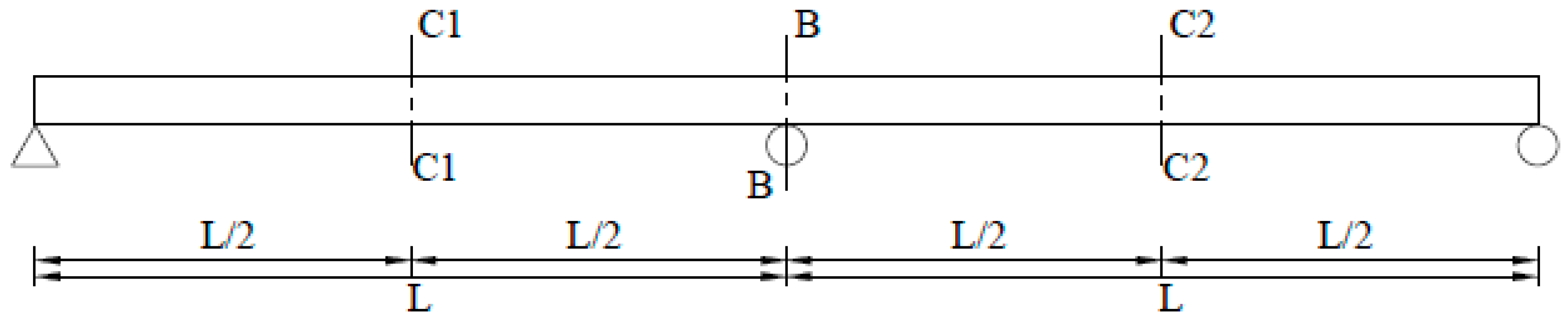
First of all, the notation employed for DAF and FDAF is clarified for the continuous beam model. Three different sections are chosen for investigating DAF of a continuous beam due to a moving vehicle (Figure 7).
Two sections, “C1-C1” and “C2-C2”, located at mid-lengths of the first and second spans, are used as a reference for sagging moments. The DAF of sagging moment at mid-length of first and second spans are denoted SDAF1 (DAF for a location “C1-C1” in Equation (8)) and SDAF2 (DAF for a location “C2-C2” in Equation (8)) respectively. Although sections C1-C1 and C2-C2 are symmetric with respect to the internal support, SDAF1 and SDAF2 can be significantly different depending on the location and magnitude of the vehicular forces (affected by road irregularities and bridge deflections) and the oscillatory inertial forces of the bridge when the maximum total response takes place. I.e., maximum dynamic amplifications will be caused if the dynamic component of the response at the section under investigation reaches a peak at the same time that the maximum static component of the response occurs.
A third DAF, labelled HDAF, is introduced to characterize the hogging bending moment over the internal support section “B-B” and it is calculated using Equation (9).
Similarly, three FDAFs are defined for the continuous beam model: FSDAF1, FSDAF2 and FHDAF. FSDAF1 means the ratio of the maximum Total Sagging Bending Moment (TSBM) across the full first span length to the maximum static sagging bending moment at section C1-C1. The same definition applies to FSDAF2 except that the maximum TSBM refers to the full second span length and the maximum static sagging bending moment refers to section C2-C2. Meanwhile, FHDAF for hogging bending moment is the ratio of the maximum Total Hogging Bending Moments (THBM) across the entire beam length to the maximum static hogging bending moment over the internal support.
3.2.1. DAF of Sagging Moments
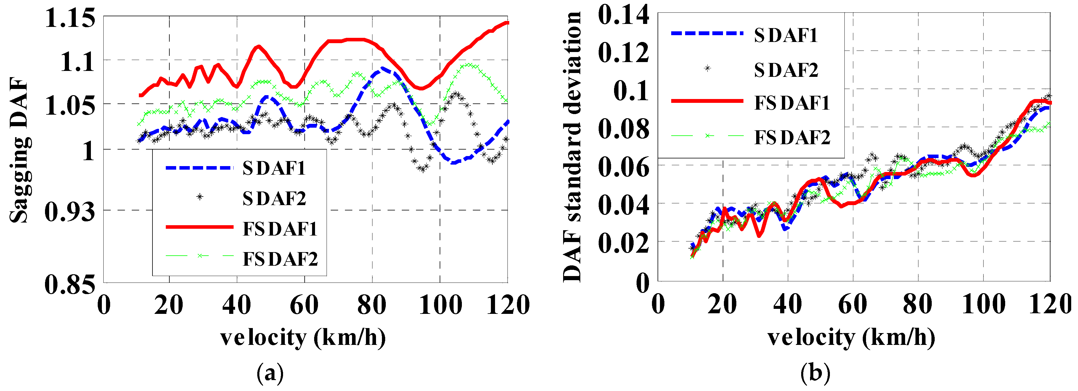
Figure 8a,b shows the mean and standard deviation respectively of SDAF/FSDAF due to the 2-axle truck on 100 class “B” road profiles. The highest mean value corresponds to FSDAF1 at 120 km/h, and it is equal to 1.14 with a standard deviation of 0.09.
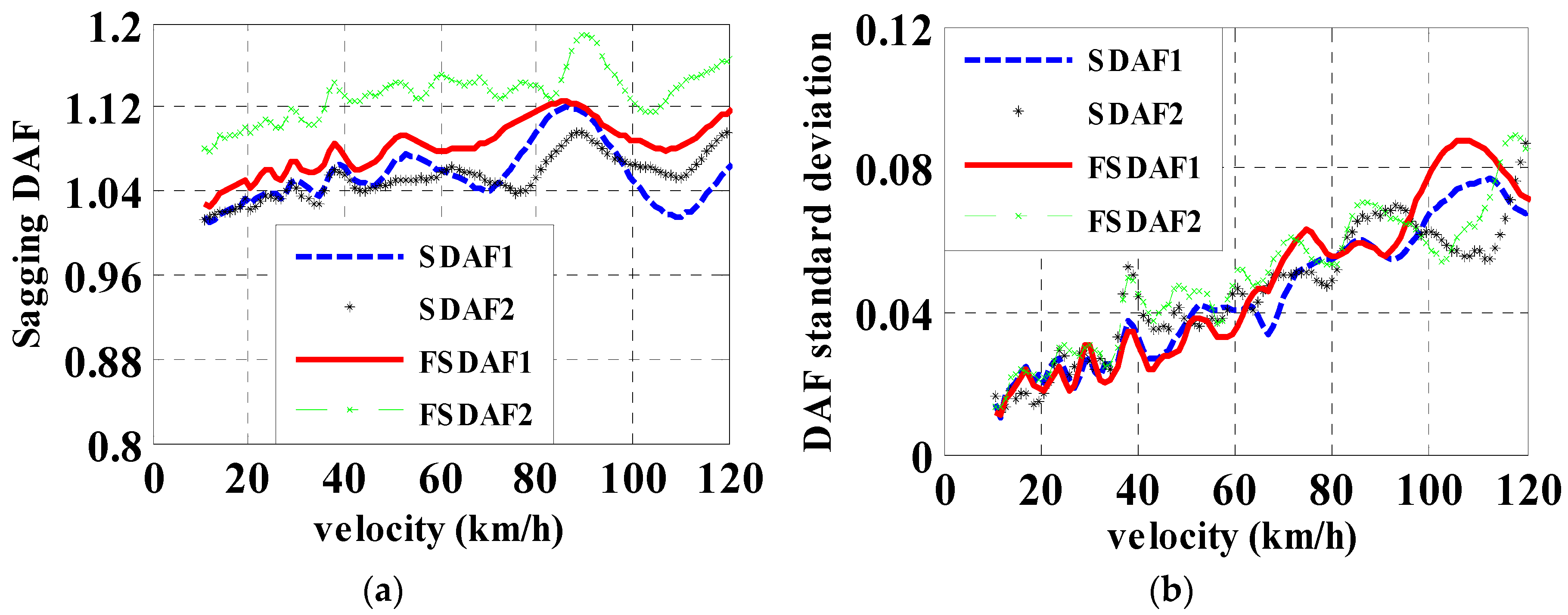
Figure 9a,b shows the mean and standard deviation respectively, of SDAF/FSDAF due to the 5-axle vehicle travelling on 100 class “B” road profiles. A highest mean dynamic amplification of 1.19 takes place for FSDAF2 at 90.72 km/h with a standard deviation of 0.07.
3.2.2. DAF of Hogging Moments
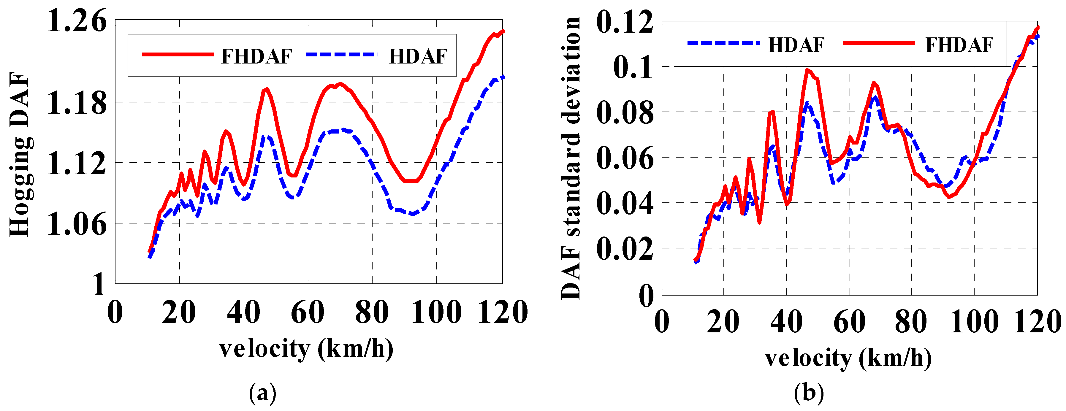
Figure 10a,b shows the mean and standard deviation respectively of HDAF/FHDAF due to the 2-axle vehicle on 100 class “B” road profiles. A highest mean FHDAF of 1.25 is found at 120 km/h with a standard deviation of 0.115.
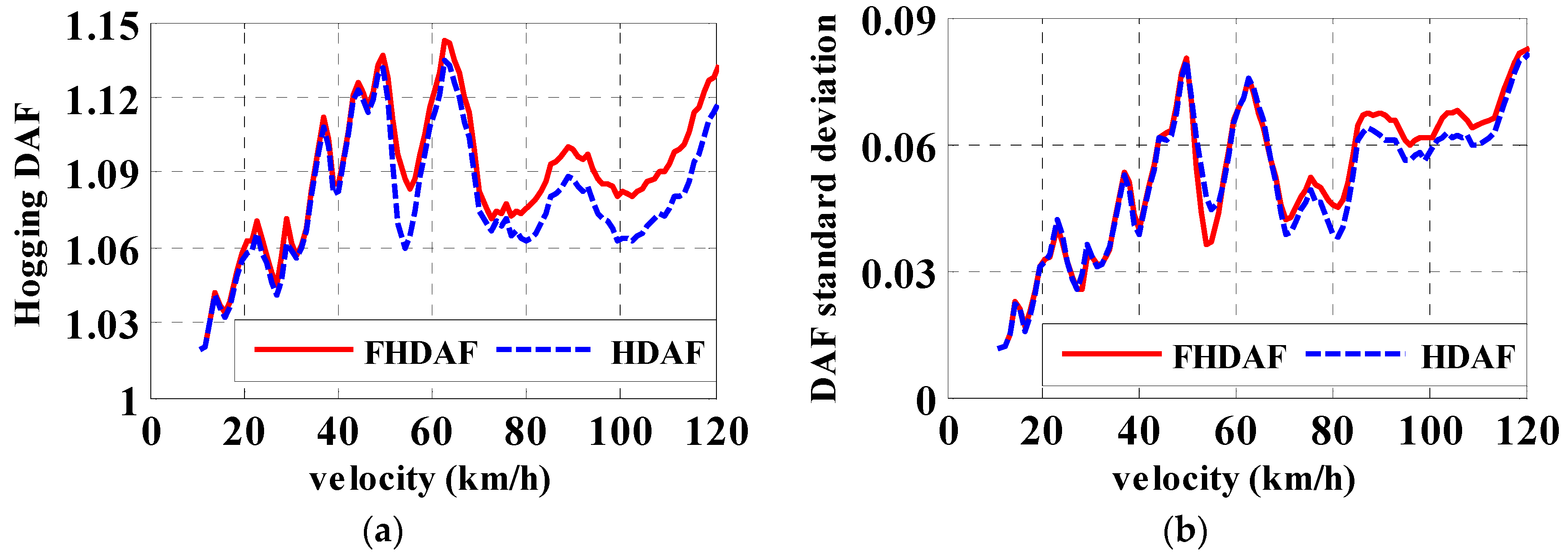
Figure 11a,b shows the mean and standard deviation of HDAF/FHDAF due to the 5-axle truck on 100 class “B” road profiles. It can be observed that a highest mean FHDAF of 1.14 occurs for 62.64 km/h with a standard deviation of 0.075.
Table 6 highlights the highest mean values for each road class and vehicle scenario. A highest mean HDAF/FHDAF of 1.06 (with a standard deviation of 0.03) appears at 36.72 km/h for the 5-axle truck travelling over a road class “A”. However, this value increases up to 1.14 for FHDAF at 62.64 km/h on a road class “B”. As expected, these values further increase for the lighter 2-axle vehicle, i.e., FHDAF of 1.25 at 120 km/h on a road class “B”.
4. Discussion
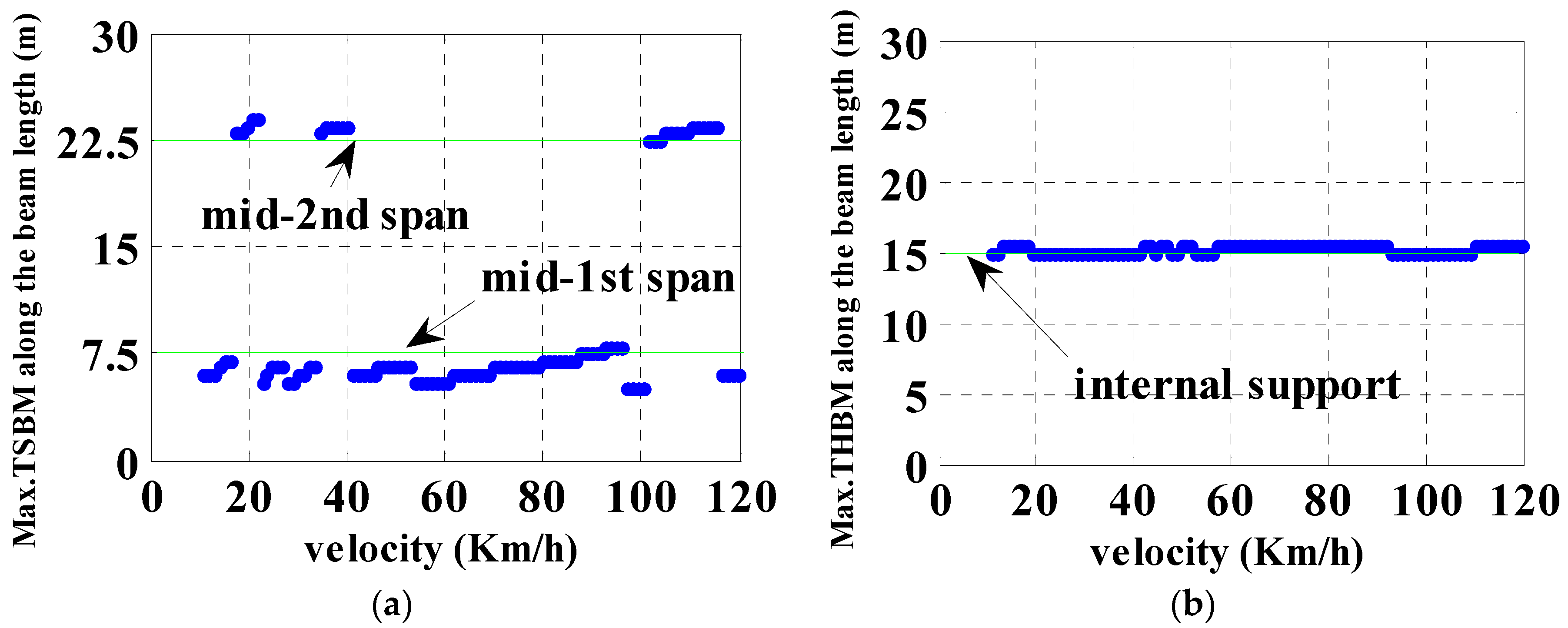
Values of DAF and FDAF generally rise when road roughness increases. In some cases, FDAFs are significantly larger than DAF. The latter is due to the fact that the location holding the maximum total moment may be different from the section taken as reference (i.e., mid-length of the span for sagging and the section over internal support for hogging). Figure 12a,b shows how the location of maximum TSBM and THBM respectively, varies with vehicle velocity for the 2-axle vehicle travelling on road class “B”. Furthermore, Figure 12a reveals that maximum TSBM usually takes place near the mid-length of the first span of the beam, although some critical locations could be far apart from the exact mid-span point or even in the second span. The location holding the maximum THBM will be the section over the internal support of the beam. The location of the maximum THBM does not experience significant variations given that the static component of hogging moment reaches a maximum over the internal support and then drops sharply in the locations nearby.
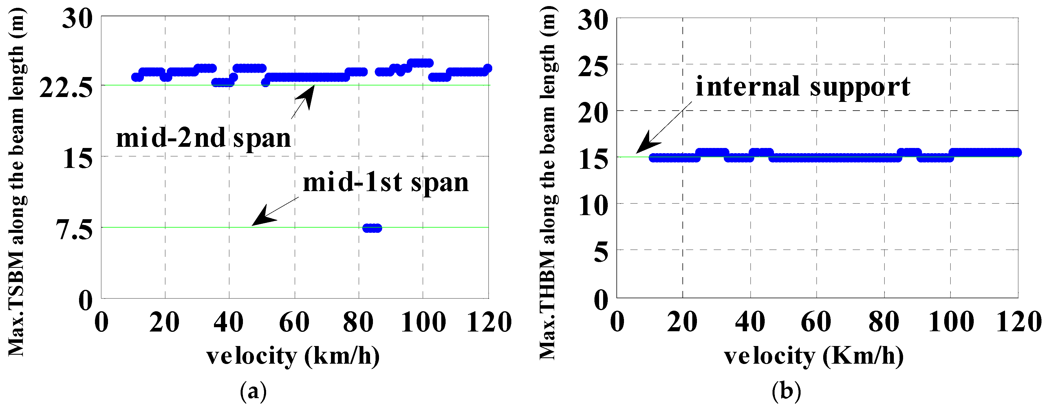
The variation of the location of the TSBM and THBM with velocity for the 5-axle vehicle is shown in Figure 13a,b respectively. Unlike the 2-axle vehicle, Figure 13a shows that the location holding the maximum TSBM is mainly situated about the mid-length of the second span. As for the 2-axle truck, Figure 13b shows that the maximum THBM is located in the section over the internal support.
Table 4, Table 5 and Table 6 have shown that vehicle configuration has a large effect on the location and magnitude of the largest moments developing in the beam. While mean FSDAF1 (=1.13 and 1.14 for classes “A” and “B” respectively) is larger than mean FSDAF2 (=1.10 and 1.09 for classes “A” and “B” respectively) for the 2-axle vehicle, mean FSDAF2 (=1.14 and 1.19 for classes “A” and “B” respectively) is larger than mean FSDAF1 (=1.10 and 1.12 for classes “A” and “B” respectively) for the 5-axle truck. Mean full dynamic amplification factor for the sagging moments (FSDAF) due the effect of 5-axle vehicle travelling over road class “B” is greater than that of the 2-axle vehicle by about 0.06. However, in the case of hogging, mean FHDAF due to the 2-axle vehicle on road class “B” is 0.09 higher than that of the 5-axle vehicle.
When comparing the full dynamic amplification factors of hogging and sagging moments, FHDAF (=1.25) is 0.12 higher than FSDAF for the 2-axle vehicle travelling over road class “B”. Meanwhile, FSDAF (=1.19) is 0.05 higher than FHDAF when the 5-axle vehicle travels over road class “B”.
If the comparison was made between the sagging response of simply supported and continuous beams due to the 2-axle vehicle over road class “B”, maximum mean FDAF and FSDAF of 1.12 and 1.14 respectively are obtained. In the case of the 5-axle vehicle over a road class “B”, the maximum mean FSDAF value (=1.19) in the continuous beam is again about 0.02 greater than the FDAF in the simply supported beam. Comparing hogging in the continuous beam and sagging in the simply supported beam with a road class “B”, the maximum FHDAF value is 0.03 lower than FDAF for the 5-axle vehicle, and 0.12 higher than the FDAF for the 2-axle vehicle. From these results, it becomes clear that it is not always safe to apply dynamic amplification factors of sagging found in single span structures to moments in continuous structures.
Finally, it is worth noting that the results reported in this paper have been obtained for a specific combination of bridge, vehicle and road characteristics. These DAF values cannot be generalized to bridges and/or vehicles with properties and/or road surface with irregularities (i.e., presence of bumps) that differ from those considered in Section 2. Therefore, a planar model has been employed in the simulations. The latter works best when resembling the response of relatively long bridges compared to their width. I.e., transverse effects have been neglected, and the reactions at the supports, the vehicle forces and the inertial forces of the bridge have been assumed to be uniformly distributed across the width. Hence, DAF values from a planar model cannot be directly applied to continuous bridges where the bridge width is significant and where the support reactions may be concentrated in a few discrete points.
5. Summary and Conclusions
This paper has compared DAF and FDAF of a continuous beam with two equal spans to those of a simply supported beam. In the continuous beam, the two mid-sections of the first and second spans have been used as a reference for calculations of DAF and FDAF for sagging moments. The section over the internal support has been selected for calculating DAF and FDAF of hogging moment. The two beam models have been traversed by two truck configurations: a rigid 2-axle and a 3-axle trailer towed by a 2-axle. The influence of the road surface has been investigated for two roughness classes: “A” (very good) and “B” (good). The critical location holding the maximum total hogging moment has typically been the section over the internal support or very close to it and as a result, DAF and FDAF of hogging yield very similar values. However, the critical location holding the maximum total sagging has been shown to vary significantly, and differences between DAF and FDAF of sagging have become more significant than in the case of hogging. A highest mean FDAF of 1.25 has been found at the maximum velocity under investigation (120 km/h), for hogging, the 2-axle vehicle and a road class “B”. Maximum FDAFs/DAFs have occurred at critical velocities that have not changed for the 2-axle vehicle when increasing the road roughness from class “A” to “B”. FDAF of sagging bending moment in continuous beam has been found to be slightly greater than FDAF of the simply supported beam for the 5-axle vehicle travelling over road class “B”. FDAF of hogging moment (=1.25) has been found to be considerably higher than FDAF of sagging moment (=1.14) when the 2-axle vehicle travels over the continuous beam with a road class “B”. When travelling on a road class “B”, FDAF of hogging moment has been reduced from 1.25 for the 2-axle vehicle to 1.14 for the 5-axle vehicle.
The current investigation, although limited to the models and parameters under consideration, has shown that DAF and FDAFs do not only depend on the vehicle configuration, the road roughness and the bridge characteristics, but also on the sign of the load effect being investigated. Evidence has been provided on the potential relevance of the dynamic increment of hogging moment over internal supports with respect to the static response. It has also been shown that dynamic amplification factors of sagging cannot be extended to hogging. The latter needs to be taken into consideration for delivering an accurate picture of the total response of continuous multi-span structures for design or assessment purposes. I.e., calculations required for ensuring the capacity of a bridge is sufficient to withstand a large heavy goods vehicle requiring a special permit should incorporate the differences in dynamic amplification associated with each load effect and section under investigation. Similarly, site-specific static traffic load models based on weight-in-motion measurements can be extended to take these variations of dynamic amplification into account.
Author Contributions
A.G. and O.M. conceived the original idea. O.M. performed the numerical simulations under the supervision of A.G. Both authors discussed the results and contributed to the final manuscript.
Acknowledgments
The authors wish to express their gratitude for the financial support received from the University of Anbar and Iraqi Ministry of Higher Education towards this research.
Conflicts of Interest
The authors declare no conflict of interest.
References
- Frýba, L. Vibration of Solids and Structures Under Moving Loads; Noordhoff International Publishing: Groningen, The Netherlands, 1972. [Google Scholar] [CrossRef]
- Cantieni, R. Dynamic Load Testing of Highway Bridges; Technical Report; Transportation Research Board: Washington, DC, USA, 1984; Volume 950, pp. 141–148. Available online: http://onlinepubs.trb.org/Onlinepubs/trr/1984/950/950v2-015.pdf (accessed on 18 May 2018).
- Green, M.F.; Cebon, D.; Cole, D.J. Effects of vehicle suspension design on dynamics of highway bridges. J. Struct. Eng. 1995, 121, 272–282. [Google Scholar] [CrossRef]
- Yang, Y.B.; Liao, S.S.; Lin, B.H. Impact formulas for vehicles moving over simple and continuous beams. J. Struct. Eng. 1995, 121, 1644–1650. [Google Scholar] [CrossRef]
- Chan, T.H.; O’Connor, C. Vehicle model for highway bridge impact. J. Struct. Eng. 1990, 116, 1772–1793. [Google Scholar] [CrossRef]
- Ichikawa, M.; Miyakawa, Y.; Matsuda, A. Vibration analysis of the continuous beam subjected to a moving mass. J. Sound Vib. 2000, 230, 493–506. [Google Scholar] [CrossRef]
- Brady, S.P.; O’Brien, E.J. Effect of vehicle velocity on the dynamic amplification of two vehicles crossing a simply supported bridge. J. Bridge Eng. 2006, 11, 250–256. [Google Scholar] [CrossRef]
- Miguel, L.F.F.; Lopez, R.H.; Torii, A.J.; Miguel, L.F.F.; Beck, A.T. Robust design optimization of TMDs in vehicle–bridge coupled vibration problems. Eng. Struct. 2016, 126, 703–711. [Google Scholar] [CrossRef]
- Paultre, P.; Chaallal, O.; Proulx, J. Bridge dynamic and dynamic amplification factors—A review of analytical and experimental findings. Can. J. Civ. Eng. 1992, 19, 260–278. [Google Scholar] [CrossRef]
- Deng, L.; Yu, Y.; Zou, Q.; Cai, C.S. State-of-the-Art review of dynamic impact factors of highway bridges. J. Bridge Eng. 2014, 20, 04014080. [Google Scholar] [CrossRef]
- Chu, V.T.H. A Self-Learning Manual Mastering Different Fields of Civil Engineering Works (VC-Q&A Method). 2010. Available online: http://civil808.com/article/ac/3428 (accessed on 18 May 2018).
- Yang, Y.B.; Yau, J.D.; Wu, Y.S. Vehicle Bridge Interaction Dynamics with Application to High-Speed Railways; World Scientific Publishing Co. Pte. Ltd.: Singapore, 2004. [Google Scholar] [CrossRef]
- Rezaiguia, A.; Ouelaa, N.; Laefer, D.F.F.; Guenfoud, S. Dynamic amplification of a multi-span, continuous orthotropic bridge deck under vehicular movement. Eng. Struct. 2015, 100, 718–730. [Google Scholar] [CrossRef]
- Cantero, D.; González, A.; O’Brien, E.J. Maximum dynamic stress on bridges traversed by moving loads. Proc. ICE Bridge Eng. 2009, 162, 75–85. [Google Scholar] [CrossRef]
- Mohammed, O.; Cantero, D.; González, A.; Al-Sabah, S. Dynamic amplification factor of continuous versus simply supported bridges due to the action of a moving load. In Proceedings of the Civil Engineering Research in Ireland (CERI 2014), Queen’s University, Belfast, Ireland, 28–29 August 2014; Available online: http://hdl.handle.net/10197/6582 (accessed on 18 May 2018).
- González, A. Vehicle-bridge dynamic interaction using finite element modelling. In Finite Element Analysis; Moratal, D., Ed.; Sciyo: Rijeka, Croatia, 2010; pp. 637–662. Available online: https://www.intechopen.com/books/finite-element-analysis/vehicle-bridge-dynamic-interaction-using-finite-element-modelling (accessed on 18 May 2018).
- O’Brien, E.; González, A.; McGetrick, P. A drive-by inspection system via vehicle moving force identification. Smart Struct. Syst. 2012, 5, 821–848. [Google Scholar] [CrossRef]
- Keenahan, J.; O’Brien, E.J.; McGetrick, P.J.; González, A. The use of a dynamic truck-trailer drive-by system to monitor bridge damping. Struct. Health Monit. 2014, 13, 143–157. [Google Scholar] [CrossRef] [Green Version]
- McGetrick, P.; Kim, C.-W.; González, A.; O’Brien, E. Experimental validation of a drive-by stiffness identification method for bridge monitoring. Struct. Health Monit. 2015, 14, 317–331. [Google Scholar] [CrossRef] [Green Version]
- European Committee for Standardization (CEN). Eurocode 1: Actions on Structures, Part 2: Traffic Loads on Bridges (EN 1991-2:2003); European Committee for Standardization: Brussels, Belgium, 2003. [Google Scholar]
- Cebon, D. Handbook of Vehicle-Road Interaction; Swets & Zeitlinger: Lisse, The Netherlands, 1999; Available online: https://www.crcpress.com/Handbook-of-Vehicle-Road-Interaction/Cebon/p/book/9789026515545 (accessed on 18 May 2018).
- Harris, N.K.; O’Brien, E.J.; González, A. Reduction of bridge dynamic amplification through adjustment of vehicle suspension damping. J. Sound Vib. 2007, 302, 471–485. [Google Scholar] [CrossRef]
- Li, Y.C. Factors Affecting the Dynamic Interaction of Bridges and Vehicle Loads. Ph.D. Thesis, Department of Civil Engineering, University College Dublin, Dublin, Ireland, 2006. [Google Scholar]
- Clough, R.W.; Penzien, J. Dynamics of Structures; McGraw-Hill: New York, NY, USA, 1993. [Google Scholar] [CrossRef]
- Wang, T.; Huang, D.; Shahawy, M. Dynamic response of multigirder bridges. J. Struct. Eng. 1992, 118, 2222–2238. [Google Scholar] [CrossRef]
- Huang, D.Z.; Wang, T.L.; Shahawy, M. Dynamic behavior of horizontally curved I-girder bridges. Comput. Struct. 1995, 57, 703–714. [Google Scholar] [CrossRef]
- Kim, C.-W.; Kawatani, M.; Kwon, Y.-R. Impact coefficient of reinforced concrete slab on a steel girder bridge. Eng. Struct. 2007, 29, 576–590. [Google Scholar] [CrossRef]
- International Organization for Standardization (ISO). Mechanical Vibration—Road Surface Profiles—Reporting of Measured Data; ISO8608 (BS7853:1996); International Organization for Standardization: Geneva, Switzerland, 1995. [Google Scholar]
- Cebon, D.; Newland, D.E. Artificial generation of road surface topography by the inverse F.F.T. method. Veh. Syst. Dyn. 1983, 12, 160–165. [Google Scholar] [CrossRef]
- Agostinacchio, M.; Ciampa, D.; Olita, S. The vibrations induced by surface irregularities in road pavements—A Matlab® approach. Eur. Trans. Res Rev. 2013, 6, 267–275. [Google Scholar] [CrossRef]
- Sayers, M.W.; Karamihas, S.M. Interpretation of Road Roughness Profile Data—Final Report; University of Michigan Transportation Research Institute (UMTRI): Ann Arbor, MI, USA, 1996. [Google Scholar]
- MATLAB, version r 2014 a; The MathWorks: Natick, MA, USA, 2014; Available online: https://aj-hub.ucd.ie/ (accessed on 18 May 2018).
- Tedesco, J.W.; McDougal, W.G.; Ross, C.A. Structural Dynamics: Theory and Applications; Addison-Wesley Longman: Petaluma, CA, USA, 1999; ISBN-10 0673980529. [Google Scholar]
Figure 1.
Vehicle models: (a) 2-axle; (b) 5-axle.

Figure 2.
Road irregularities for two random profiles with different road class: (a) Class “A”; (b) Class “B”.
Figure 2.
Road irregularities for two random profiles with different road class: (a) Class “A”; (b) Class “B”.

Figure 3.
Static and total Bending Moment (BM) response of continuous beam due to the effect of the two-axle truck: (a) sagging moment at mid-length of the 1st span; (b) hogging moment over the internal support.
Figure 3.
Static and total Bending Moment (BM) response of continuous beam due to the effect of the two-axle truck: (a) sagging moment at mid-length of the 1st span; (b) hogging moment over the internal support.

Figure 4.
DAF/FDAF due to the 2-axle vehicle on road class “B”: (a) mean; (b) standard deviation.

Figure 5.
DAF/FDAF due to the 5-axle vehicle on road class “B”: (a) mean; (b) standard deviation.

Figure 6.
Location of maximum total bending moment (TBM) along the simply supported beam due to the crossing of: (a) 2-axle vehicle; (b) 5-axle vehicle.
Figure 6.
Location of maximum total bending moment (TBM) along the simply supported beam due to the crossing of: (a) 2-axle vehicle; (b) 5-axle vehicle.

Figure 7.
Location of sections of a continuous beam taken as reference for DAF calculations.

Figure 8.
SDAF/FSDAF due to the 2-axle vehicle on road class “B”: (a) mean; (b) standard deviation.

Figure 9.
SDAF/FSDAF due to the 5-axle vehicle on road class “B”: (a) mean; (b) standard deviation.

Figure 10.
HDAF/FHDAF due to the 2-axle vehicle on road class “B”: (a) mean; (b) standard deviation.
Figure 10.
HDAF/FHDAF due to the 2-axle vehicle on road class “B”: (a) mean; (b) standard deviation.

Figure 11.
HDAF/FHDAF due to the 5-axle vehicle on road class “B”: (a) mean; (b) standard deviation.
Figure 11.
HDAF/FHDAF due to the 5-axle vehicle on road class “B”: (a) mean; (b) standard deviation.

Figure 12.
Location of maximum total bending moment along the continuous beam versus velocity for 2-axle vehicle: (a) Sagging (TSBM); (b) hogging (THBM).
Figure 12.
Location of maximum total bending moment along the continuous beam versus velocity for 2-axle vehicle: (a) Sagging (TSBM); (b) hogging (THBM).

Figure 13.
Location of maximum total bending moment (along the continuous beam versus velocity for 5-axle vehicle: (a) sagging (TSBM); (b) hogging (THBM).
Figure 13.
Location of maximum total bending moment (along the continuous beam versus velocity for 5-axle vehicle: (a) sagging (TSBM); (b) hogging (THBM).


Table 1.
2-axle truck properties (4 DOFs).
| Property | Symbol | Value | Unit |
|---|---|---|---|
| Body Mass | ms | 26,750 | kg |
| Axle1 mass | mu1 | 700 | kg |
| Axle2 mass | mu2 | 1100 | kg |
| Suspension stiffness | Ks1 | 4 × 10⁵ | N m−1 |
| Ks2 | 10 × 105 | N m−1 | |
| Suspension Damping | Cs1 | 10 × 103 | Ns m−1 |
| Cs2 | 20 × 103 | Ns m−1 | |
| Tire Stiffness | Kt1 | 1.75 × 10⁶ | N m−1 |
| Kt2 | 3.5 × 10⁶ | N m−1 | |
| Tire Damping | Ct1 | 3 × 10³ | Ns m−1 |
| Ct2 | 5 × 10³ | Ns m−1 | |
| Moment of Inertia | Is | 154,320 | kg m2 |
| Body bounce frequency | fbounce | 0.86 | Hz |
| Body pitch frequency | fpitch | 1.02 | Hz |
| Axle1 hop frequency | faxle1 | 8.83 | Hz |
| Axle2 hop frequency | faxle2 | 10.19 | Hz |
Table 2.
5-axle truck trailer properties (9 DOFs).
| Property | Symbol | Value | Unit |
|---|---|---|---|
| Body Mass 1 | ms1 | 25,200 | kg |
| Body Mass 2 | ms2 | 30,700 | kg |
| Axle1 mass | mu1 | 700 | kg |
| Axle2 mass | mu2 | 1100 | kg |
| Axle3 mass | mu3 | 1100 | kg |
| Axle4 mass | mu4 | 1100 | kg |
| Axle5 mass | mu5 | 1100 | kg |
| Suspension stiffness | Ks1 | 4 × 10⁵ | N m−1 |
| Ks2, Ks3, Ks4, Ks5 | 10 × 105 | N m−1 | |
| Suspension Damping | Cs1 | 10 × 103 | Ns m−1 |
| Cs2, Cs3, Cs4, Cs5 | 20 × 103 | Ns m−1 | |
| Tire Stiffness | Kt1 | 1.75 × 10⁶ | N m−1 |
| Kt2, Kt3, Kt4, Kt5 | 3.5 × 10⁶ | N m−1 | |
| Tire Damping | Ct1 | 3 × 10³ | Ns m−1 |
| Ct2, Ct3, Ct4, Ct5 | 5 × 10³ | Ns m−1 | |
| Moment of Inertia 1 | Is1 | 86,410 | kg m2 |
| Moment of Inertia 2 | Is2 | 112,440 | kg m2 |
| Body 1 bounce frequency | f1bounce | 1.56 | Hz |
| Body 1 pitch frequency | f1pitch | 2.39 | Hz |
| Axle1 hop frequency | faxle1 | 9.97 | Hz |
| Axle2 hop frequency | faxle2 | 8.77 | Hz |
| Body 2 bounce frequency | f2bounce | 2.12 | Hz |
| Body 2 pitch frequency | f2pitch | 2.33 | Hz |
| Axle3 hop frequency | faxle3 | 10.03 | Hz |
| Axle4 hop frequency | faxle4 | 10.15 | Hz |
| Axle5 hop frequency | faxle5 | 10.17 | Hz |
Table 3.
Highest mean value (µ) and standard deviation (σ) of DAF in the simply supported beam with road classes “A” and “B”.
Table 3.
Highest mean value (µ) and standard deviation (σ) of DAF in the simply supported beam with road classes “A” and “B”.
| Vehicle Type | Class Type of Road Surface | |||||||||||
|---|---|---|---|---|---|---|---|---|---|---|---|---|
| Class “A” | Class “B” | |||||||||||
| DAF | FDAF | DAF | FDAF | |||||||||
| µ | σ | Velocity km/h | µ | σ | Velocity km/h | µ | σ | Velocity km/h | µ | σ | Velocity km/h | |
| 2-axle | 1.12 | 0.036 | 85.32 | 1.12 | 0.036 | 85.32 | 1.12 | 0.065 | 85.32 | 1.12 | 0.065 | 85.32 |
| 5-axle | 1.12 | 0.04 | 93.6 | 1.14 | 0.04 | 91.8 | 1.14 | 0.07 | 91.8 | 1.17 | 0.07 | 92.88 |
Table 4.
Highest mean value (µ) and standard deviation (σ) of FSDAF/SDAF in the continuous beam with road class “A”.
Table 4.
Highest mean value (µ) and standard deviation (σ) of FSDAF/SDAF in the continuous beam with road class “A”.
| Vehicle Type | SDAF1 | SDAF2 | FSDAF1 | FSDAF2 | ||||||||
|---|---|---|---|---|---|---|---|---|---|---|---|---|
| µ | σ | Velocity km/h | µ | σ | Velocity km/h | µ | σ | Velocity km/h | µ | σ | Velocity km/h | |
| 2-axle | 1.1 | 0.04 | 83.11 | 1.08 | 0.04 | 105.8 | 1.13 | 0.06 | 120 | 1.1 | 0.04 | 108 |
| 5-axle | 1.09 | 0.03 | 85.32 | 1.05 | 0.04 | 101.5 | 1.1 | 0.03 | 84.24 | 1.14 | 0.04 | 90.72 |
Table 5.
Highest mean value (µ) and standard deviation (σ) of FSDAF/SDAF in the continuous beam with road class “B”.
Table 5.
Highest mean value (µ) and standard deviation (σ) of FSDAF/SDAF in the continuous beam with road class “B”.
| Vehicle Type | SDAF1 | SDAF2 | FSDAF1 | FSDAF2 | ||||||||
|---|---|---|---|---|---|---|---|---|---|---|---|---|
| µ | σ | Velocity km/h | µ | σ | Velocity km/h | µ | σ | Velocity km/h | µ | σ | Velocity km/h | |
| 2-axle | 1.09 | 0.07 | 84.24 | 1.06 | 0.07 | 104.8 | 1.14 | 0.09 | 120 | 1.09 | 0.07 | 108 |
| 5-axle | 1.12 | 0.06 | 87.48 | 1.1 | 0.07 | 88.56 | 1.12 | 0.06 | 85.32 | 1.19 | 0.07 | 90.72 |
Table 6.
Highest mean value (µ) and standard deviation (σ) in FHDAF/HDAF of the continuous beam with road classes “A” and “B”.
Table 6.
Highest mean value (µ) and standard deviation (σ) in FHDAF/HDAF of the continuous beam with road classes “A” and “B”.
| Vehicle Type | Class “A” | Class “B” | ||||||||||
|---|---|---|---|---|---|---|---|---|---|---|---|---|
| HDAF | FHDAF | HDAF | FHDAF | |||||||||
| µ | σ | Velocity km/h | µ | σ | Velocity km/h | µ | σ | Velocity km/h | µ | σ | Velocity km/h | |
| 2-axle | 1.11 | 0.06 | 120 | 1.15 | 0.07 | 120 | 1.2 | 0.11 | 120 | 1.25 | 0.11 | 120 |
| 5-axle | 1.06 | 0.03 | 36.76 | 1.06 | 36.72 | 0.03 | 1.13 | 0.07 | 62.64 | 1.14 | 0.07 | 62.64 |
© 2018 by the authors. Licensee MDPI, Basel, Switzerland. This article is an open access article distributed under the terms and conditions of the Creative Commons Attribution (CC BY) license (http://creativecommons.org/licenses/by/4.0/).
Share and Cite
MDPI and ACS Style
González, A.; Mohammed, O. Dynamic Amplification Factor of Continuous versus Simply Supported Bridges Due to the Action of a Moving Vehicle. Infrastructures 2018, 3, 12. https://doi.org/10.3390/infrastructures3020012
AMA Style
González A, Mohammed O. Dynamic Amplification Factor of Continuous versus Simply Supported Bridges Due to the Action of a Moving Vehicle. Infrastructures. 2018; 3(2):12. https://doi.org/10.3390/infrastructures3020012
Chicago/Turabian StyleGonzález, Arturo, and Omar Mohammed. 2018. "Dynamic Amplification Factor of Continuous versus Simply Supported Bridges Due to the Action of a Moving Vehicle" Infrastructures 3, no. 2: 12. https://doi.org/10.3390/infrastructures3020012