Modeling Determinants of Urban Growth in Conakry, Guinea: A Spatial Logistic Approach

1
Graduate School of Environmental Science, Hokkaido University, Sapporo, Hokkaido 060-0810, Japan
2
Faculty of Environmental Earth Science, Hokkaido University, Sapporo, Hokkaido 060-0810, Japan
*
Author to whom correspondence should be addressed.
Urban Sci. 2017, 1(2), 12; https://doi.org/10.3390/urbansci1020012
Submission received: 10 March 2017
/
Revised: 1 April 2017
/
Accepted: 6 April 2017
/
Published: 10 April 2017
Abstract
:The main objective of the present study was to integrate a logistic regression model (LRM), a geographic information system (GIS) and remote sensing (RS) techniques to analyze and quantify urban growth patterns and investigate the relationship between urban growth and various driving forces. Landsat images from 1986, 2000, and 2016 derived from the TM, ETM+, and OLI sensors respectively were used to simulate an urban growth probability map for Conakry. To better explain the effects of the drivers on the urban growth processes in the study area, variables for two groups of drivers were considered: socioeconomic proximity and physical topography. The results of the LRM using IDRISI Selva indicated that the variables elevation () and distance to major roads resulted in models with the best fit and the highest regression coefficients. These results indicate a high probability of urban growth in areas with high elevation and near major roads. The validation of the model was conducted using the relative operating characteristic (ROC) method; which result exhibited high accuracy of 0.89 between the simulated urban growth probability map and the actual one. A land use/land cover (LULC) change analysis showed that the urban area had undergone continuous growth over the study period resulting in an extent of 143.5 km2 for the urban area class in 2016.
1. Introduction
The process of urbanization has been traditionally associated with other important economic and social transformations, resulting in greater geography mobility, lower fertility, longer life expectancy and population ageing [1]. Cities are important drivers of development and poverty reduction in both urban and rural areas, as they concentrate much of the national economic activity, government, commerce, and transportation, and provide crucial links with rural areas, between cities, and across international borders. Urban living is often associated with a higher level of literacy and education, better health, greater access to social services, and enhanced opportunities for cultural and political participation. Nevertheless, in developing countries, rapid demographic and uncontrolled urban expansion have exceeded the capability of most cities for appropriate management [2]. City growth and changes in land-use patterns have various important social and environmental impacts, including the loss of natural spaces, increased vehicular congestion, urban heat island effects, landscape fragmentation and homogenization, the loss of highly productive agricultural lands, alterations in natural drainage systems, and reduced water quality [3]. To understand the spatial and temporal dynamics of these processes, the factors that drive urban growth must be identified and examined, especially those factors that can be used to predict future changes and their potential environmental effects [4].
Conakry, the capital of the Republic of Guinea, has experienced the highest population growth in the country, averaging 6.1% annually. The city’s population was estimated at nearly 2 million in 2014 [5]. This explosive population growth was accompanied by geographical expansion, with the city more than quadrupling in size since the country declared independence in 1958 [6]. The distribution of cities throughout the country’s territory is balanced, but the hierarchy of cities is very unbalanced as there is no other city counterbalancing the attraction of Conakry. Almost half of the country’s urban population resides in Conakry, which has 15 times the population of Kankan, the second-largest city in the country [7]. Conakry’s small land area and relative isolation from the mainland have created an infrastructural burden since independence, showing a great imbalance in the urban network. Urban growth in Conakry largely reflects the problems and shortcomings of Guinea’s overall economic development since independence, and has taken place with very little urban development planning or control [8]. The authorities in charge of urban planning and management have faced increasing difficulties to plan for spatial expansion and land development, to identify, coordinate and carry out the most critically needed investments in basic infrastructure and services, and to ensure proper maintenance of existing assets. Inadequate urban planning and management have led to massive, uncontrolled urban expansion. The city has become critically overcrowded, creating considerable pressure on scarce basic urban services and resulting in drastic degradation of the environment. As in many developing countries, Conakry has been faced with unprecedented urbanization issues caused by unplanned urbanization processes such as emergence of slums on coastal banks, poverty and mobility, deterioration of the road surfaces, air and water pollution, deficient solid waste collection and disposal, recurrent flooding during the rainy seasons in many parts of the city, and the alteration in climate patterns. At present, urban growth is one of the most widely discussed issues in urban studies [9]. The encroachment of urban land on non-urban land has become a common phenomenon throughout developing countries, and its impact has attracted increasing attention from planners, researchers and policy makers [10]. However, there are few studies of urban growth in Guinea, including in Conakry.
Studying and monitoring urban growth dynamics has become easier due to enormous developments in the fields of geographic information system (GIS) and remote sensing (RS) resulting in powerful tools to predict and model urban growth [11,12]. Due to the advances in spatial analysis, (GIS), and (RS) techniques, extensive efforts have been undertaken to analyze the complex spatial patterns of urban landscape changes and to understand the underlying factors using spatially explicit models [13]. Evidence has shown that applying spatial statistical models to urban expansion not only contributes to the understanding of the complex urbanization process; but also offers valuable information for environmental risk assessment [14]. Several scholars have used various empirical and theoretical modeling techniques, one of which is the logistic regression model (LRM). The application of an LRM for urban growth modeling results in an improved understanding of the urbanization process, and provides a clear picture of the weight of the explanatory variables and their respective functions [15]. LRMs also enables the integration of socioeconomic, demographic and topography factors which are not feasible in many models [16]. Based on this background, this study has integrated an LRM, GIS, and RS approach to analyze and quantify the urban growth patterns in Conakry from 1986 to 2016 and examine the relationship between urban growth and various explanatory variables.
2. Materials and Methods
2.1. Study Area
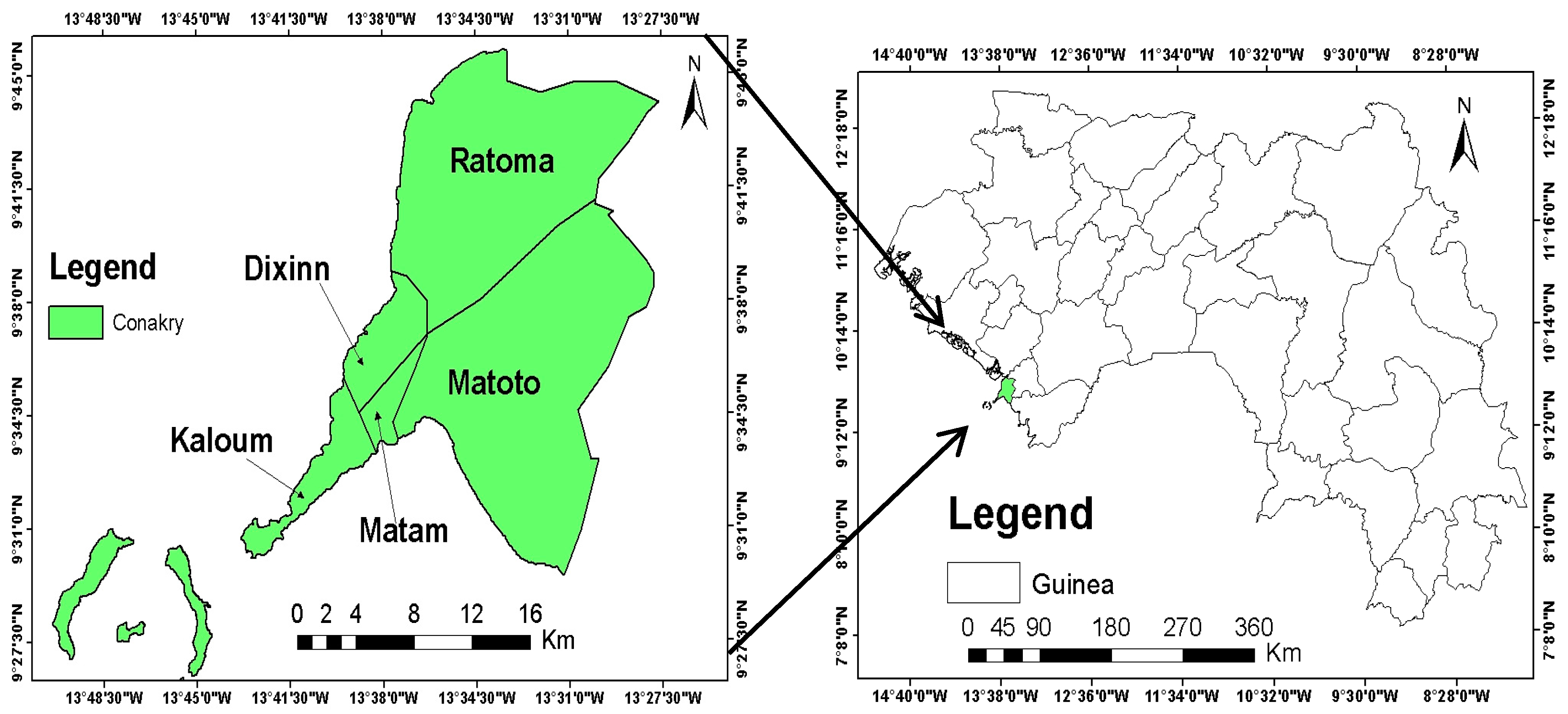
The study area consists of Conakry city, which is located in the maritime region of the Republic of Guinea (Figure 1). The city covers area extending from 9°31'N to 9°51'N latitude and from 13°42'W to 13°70'W longitude. The geographical area of Conakry is around 420 km2, which is relatively small and represents only 1% of the country’s area [17]. Conakry is divided into five communes: (1) Kaloum, which includes the major islands and the city’s economic and administrative center, (2) Dixinn, which includes the university of Conakry and many embassies, (3) Ratoma, (4) Matam, and (5) Matoto, the location of Conakry’s international airport. The city of Conakry originated in the small Tombo Island and spread up the Kaloum peninsula, sandwiched between mangrove swamps. More than 20 rivers originate inside the city’s borders, contributing to its relatively high precipitation. Mangroves line much of Conakry’s coast, a United Nations Environment Programme (UNEP) report issued in 2008 outlined the growing pressure placed on these forests by the local population, especially after an influx of refugees from Liberia and Sierra Leone in the 1990s [6]. The area of the city was originally covered by a dense tropical mangrove forests, but compared with the rest of the Guinean territories, the landscape patterns have changed considerably in recent years with substantial reduction in vegetation cover due primarily to the expansion of residential land, the felling of trees to produce charcoal, the use of forests as pastures by livestock owners during the dry season, and general deforestation [18]. Conakry’s economy revolves largely around the port, which has moderne facilities for handling and storing cargo, mainly, aluminum and bananas. Slash-and burn agricultural practices along the coastal bank, fishing and commerce are the principal activities of the residents. The climate is tropical is characterized by two alternating seasons (dry and wet). The wet season lasts from June to October and the dry season from December to April. The vegetation consists of mangroves in the marshy zone, forests of palm trees, coconuts, and some grasslands. The terrain is characterized by estuaries and littoral plains and is dominated by cliffs and the Kakoulima Mountain Range, which reaches a height of 1007 m and is located 60 km north–east of Conakry.
2.2. Data and Methods
The data used in this study were collected from various sources. First, Landsat images from different sensors, Thematic Mapper (TM) acquired on 3 January 1986, Enhanced Thematic Mapper (ETM+) on 19 December 2000, and Operational Land Imager (OLI) on 20 January 2016, were downloaded from the United States Geological Survey (USGS) and were used as primary data. Subsequently, auxiliary data were obtained by downloading from other geospatial data sources and by digitization as shown in Table 1. The study area was extracted from the temporal imagery by overlaying the boundary of the city. ArcMap10.2 GIS software was used for the different stages of images processing; namely pre-processing, generating classified land use/land cover (LULC) maps, and conducting the spatial analysis. For the image classification process, a maximum likelihood classification (MLC), which is a supervised classification method,was used for the three images by selecting appropriate polygons as training sites. The satellite images were classified into four LULC types: (1) Urban, (2) Water, (3) Vegetation, and (4) Bare ground. The accuracy of the classification was assessed by using ground control points collected during the fieldwork and obtained from Google Earth archive images. The accuracy of each classified image greater than 80%. All the data used in this study were geometrically referenced to the WGS 1984, UTM zone 28 projection systems. Subsequently, thematic raster maps of all variables were created in Arc Map 10.2 with a grid cell size of 30 m × 30 m. Finally, these raster data were converted into ASCII format for further use in the IDRISI Selva GIS software for LRM calibration and validation.
3. Logistic Regression Model
The use of LRM is one of the most popular approaches to modeling, and can be used for explaining the relationship of a number of explanatory variables to a dichotomous single dependent variable , which represents the occurrence or non-occurrence of an event [19]. Logistic regression analysis determines the relationship between the explanatory variables and the probability of the occurrence of an event [20]. The LRM also describes the effects of several factors [21]. The use of this model can determine the coefficients of the explanatory variables (both continuous and categorical), whereas the dependent variable is a binary categorical variable [22]. The value of the binary dependent variable is either 1 or 0; and can be computed by using the well-known logistic regression equation [23]. The model gives the probability of the existence or the nonexistence of each type of LULC change at every location based on the driving factors, and quantifies the interaction between the different land use types and their drivers [24]. LRM takes the following form:
where is the explanatory variable, and is a linear combination function of the explanatory variables. The parameter represents the regression coefficient to be estimated. The can be tranformed back to the probability that
The typical logistic model can effectively explain the determinants of urban land conversion.
3.1. Dependent Variable
In this study, LRM was used to model the probability of change from a non-urban to an urban land use type. The dependent variable is a dummy variable with values of 0 representing no change and 1 representing change, respectively. The urban growth that occurred between the periods of (1986–2000) and (2000–2016) was considered as dependent variable (Figure 2). Hence, a boolean image with the categories non-urban growth (cells remained unchanged) to urban growth (cells changed) was created. To generate these spatial growth maps, the raster calculator function in ArcMap10.2 was used to compute the urban growth between 1986 and 2000 and 2000 and 2016, respectively. The urban growth between 1986 and 2000 was used in the calibration phase of the LRM and for examining the relationship between the urban growth and different drivers, while the urban growth between 2000 and 2016 was used to simulate the urban growth probability map and to validate the model.
3.2. Explanatory Variables of Urban Growth
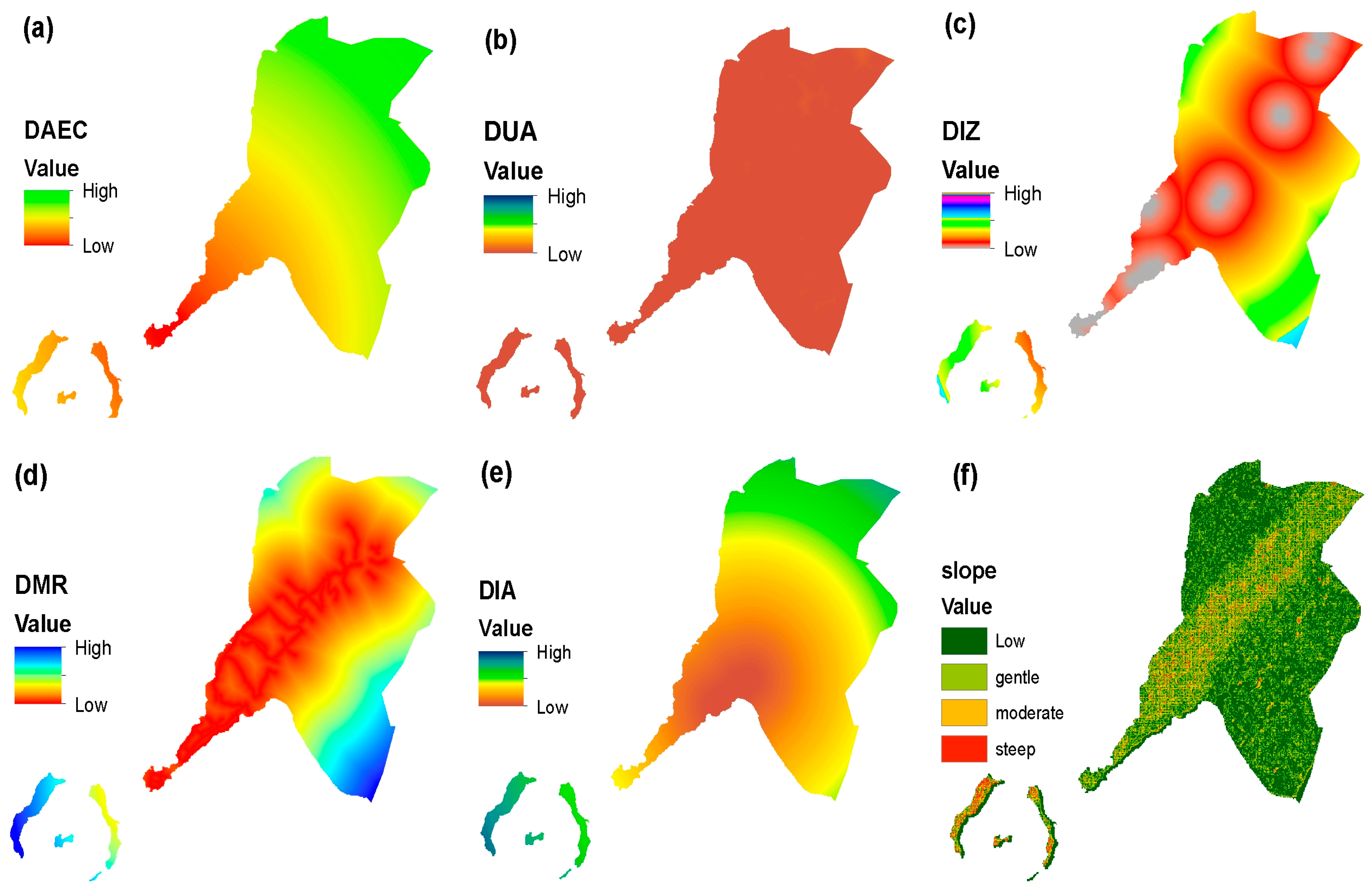
The selection of the urban growth drivers is a crucial aspect of urban growth modeling, because land use drivers are the main characteristics that can help to understand the processes of land use transition from non-urban to urban. There is no hard and fast rule or known global formula for selecting land use drivers. Therefore, the list of land use drivers can be endless [25]. Based on a literature review, field survey and personal communications with members of the urban planning bureau (UPB) in Conakry, the drivers of the urban growth in the study area were summarized into two categories. Socioeconomic proximity, and landscape topography (Table 2). The distances to active economic center (= DAEC), to the urbanized area (= DUA), to industrial zones (= DIZ), to major roads (= DUA), and to international airport (= DIA) were selected as socioeconomic proximity variables, while slope and elevation as topography variables. The distance in this study refers to the Euclidean distance in the raster image between each cell and the nearest cell of the target features. The distance variables were computed in ArcMap10.2 using a distance operator, and were converted into ASCII format prior to import into IDRISI Selva for model calibration. The slope and elevation data were extracted from the digital elevation map (Aster DEM). The slope variable was generated in percentage format, then reclassified into four categories based on the topographic charateristics of the study area: 0–2: low slope, 2–5: gentle slope, 5–9: moderate slope, 9–10: steep slope. However, there was a high discrepancy in terms of the data range between the proximity distance variables and the topographic variables. Therefore, the distance variables were normalized to a range of 0.1 to 10 before including them into the model. This process is particularly critical when an LRM is applied; since it requires that the variables are linearly related to the dependent variable. A natural log transformation was performed for the continuous distance variables; because the natural log transformation is commonly effective in linearizing distance decay variable. The Variable Transformation Utility in IDRISI Selva was used and applied to all distance variable.
3.3. Multicollinearity Analysis of the Explanatory Variables
A correlation test was conducted among the explanatory variables to check for multicollinearity. Multicollinearity describes a situation in which two or more explanatory variables are highly; linearly correlated. Perfect multicollinearity exists if the correlation between two or more explanatory variables is equal to 1 or −1 [26]. One consequence of multicollinearity is that the standard errors of the affected coefficients tend to be large. In that case, the test of the hypothesis that the coefficient is equal to zero may lead to a failure to reject a false null hypothesis of no effect of the explanatory variable. In this study, using a Pearson’s correlation coefficient and the variance inflation factors (VIF) assessed the multicollinearity test among the explanatory variables. The Pearson’s correlation coefficient has shown that the highest correlation coefficient of 0.75; which was observed between distance to industrial zones (DIZ), and distance to major roads (DMR). This high correlation occurred due to the fact that the major roads are directly related to the establishment of the industrial zones. Generally, a little bit of multicollinearity is not necessarily a huge problem, but severe multicollinearity is a major problem, because it theorically shoots up the variance of the regression coefficients, making them unstable [27]. Additionally, the VIF is another statistical approach to check for the presence of the multicollinearity in the regression analysis; and it has been used in many studies [28,29]. For determining the presence of multicollinearity using the VIF technique, the general rules of thumb is that, values of VIF should not exceed 10 [30]. According to the result shown in Table 3, there was no severe multicollinerity problem.
3.4. Statistical Test for Association between Dependent and Explanatory Variables: Cramer’s V Test
The Cramer’s V test measures the association between two nominal variables, giving a value between 0 and +1. The explanatory test procedure is based on a Cramer’s V contingency table analysis, which can test the strength of the association between the dependent variable (in this case, urban growth for the period of (1986–2000) and the explanatory variables. The test was performed using the explanatory variable test procedure in IDRISI Selva. Variables with a Cramer’s V value of about 0.15 or higher are good while those with values of 0.4 or higher are very good [31]. We found a high-strength association between Cramer’s V and some explanatory variables (Table 4). However, the LRM can explain more explicitly the association between these variables and the dependent variable.
3.5. Model Validation Using the ROC Technique
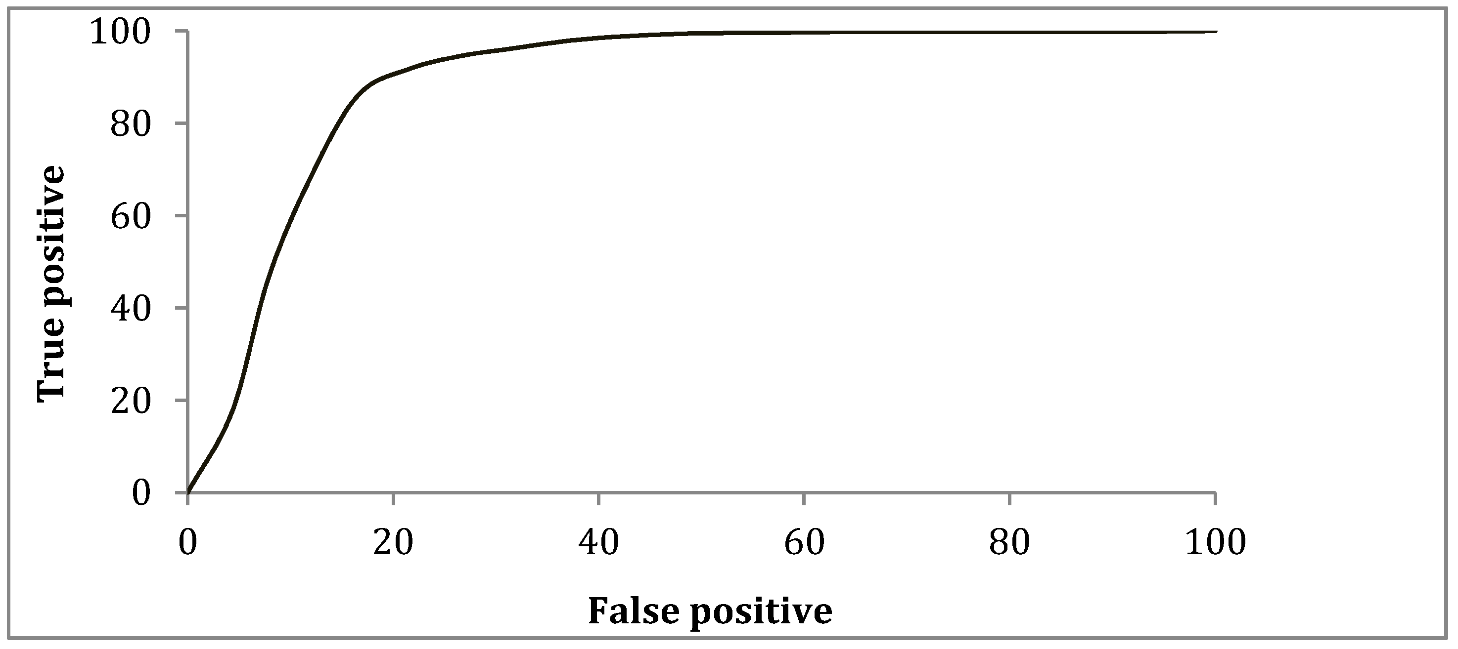
The ROC method is excellent for assessing the validity of a model that predicts the location of the occurrence of a class by comparing a suitability image depicting the likelihood of that class occurring. This method has been applied in LULC modeling studies and is considered a reliable method to validate models [32]. It calculates the percentages of false-positives and true positives for a range of thresholds or cut-off values, relating them in a chart. The ROC computes the area under the curve, which varies between 0.5 and 1.0. A value of 0.5 indicates a random assignment of the probabilities, indicating that the expected agreement is due to chance, while a value of 1.0 indicates a perfect assignment of probability. It has been shown that an ideal spatial agreement can exist between the actual urban growth and the predicted urban growth probability map [33]. In our study, the model validation was conducted by comparing the simulated urban growth probability map for 2016 with the actual growth map of 2016 using random samples of 5000 cells in the two maps. The ROC curve is based on several two-by-two contingency tables. The contingency table is based on the comparison between the actual and the predicted probability image. Table 5 shows the contingency table. ‘A’ is the number of true positive cells; which are predicted as urban growth and agree with the actual image. ‘B’ is the number of false positive cells; predicted as urban growth but disagreeing with the actual image. ‘C’ is the amount of false negative cells; which are predicted as non-urban growth but disagree with the actual map. ‘D’ is the number of true negative; cells, which are predicted as non-urban growth and agree with the actual image. From every contingency table, a single data point (x, y) is created, where x and y are the rate of false positives and the rate of true positives, respectively.
(True positive %) = A/(A + C)
(False positive %) = B/(B + D)
Those data points are joined to form the ROC curve, from which the ROC value is computed. The ROC curve is illustrated in Figure 3. The ROC value shows 0.89% of the area under the curve (AUC), indicating high agreement between the predicted and the actual urban growth map.
4. Results
4.1. LULC Change Analysis
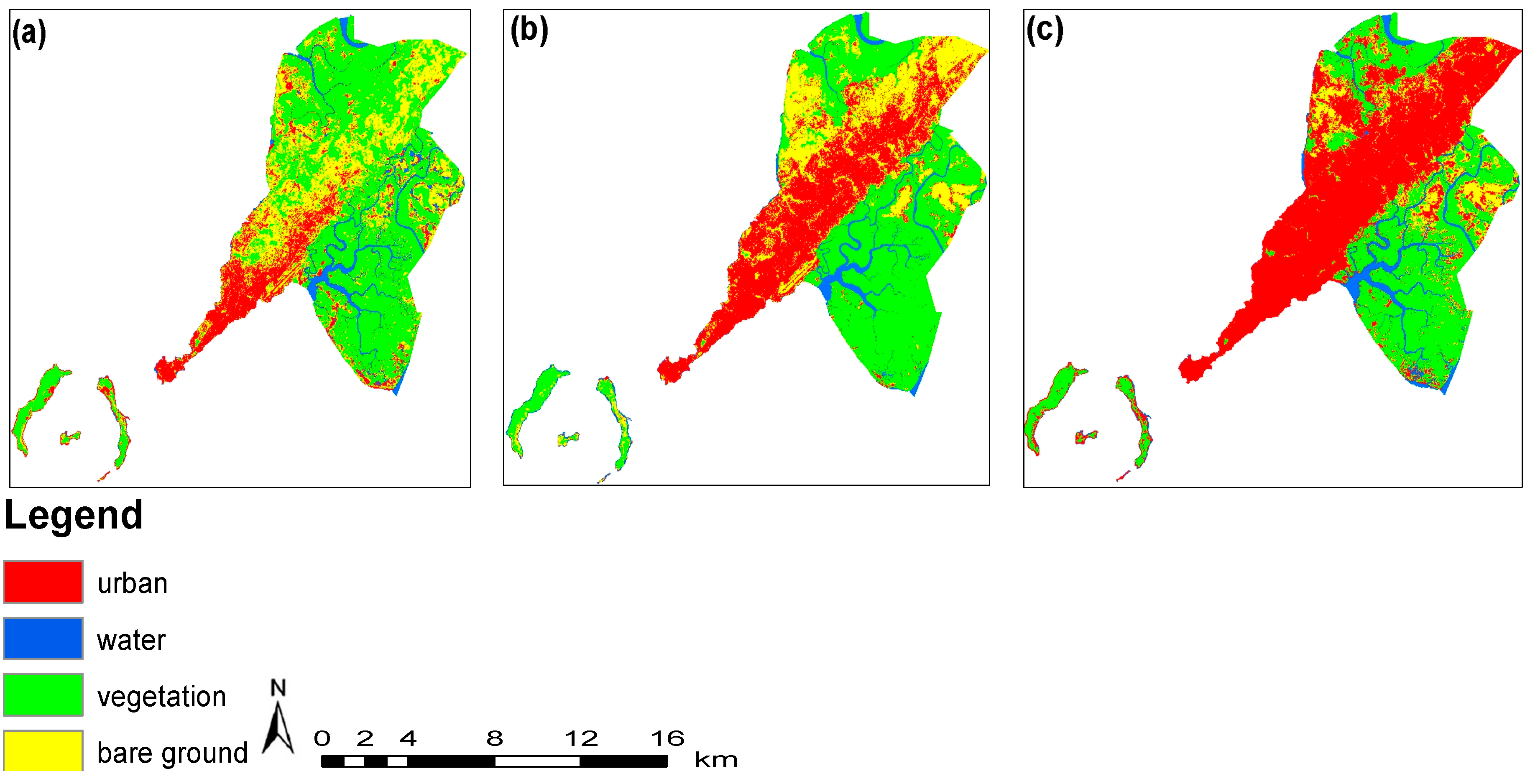
Figure 4 and Table 6 show the LULC change maps and the changes in area, respectively. As it can be observed from Table 6, the vegetation cover appeared to be the most dominant land cover type with an area of 217.48 km2 representing 51% of the total land area in 1986. The urban area class represents only 63.03 km2 in the same period. However, from 2000 to 2016, the urban land cover has sharply increased to reach 206.58 km2, which represents 49% of the total area. Bare ground decreased over the study period from 114.76 km2 in 1986 to 92.49 km2 in 2000, and to 39.88 km2 in 2016. A water class showed almost no change in its area over the study period. For more representation of the LULC changes in the study area, Figure 5 shows the changing pattern from 1986 to 2016.
4.2. Logistic Regression Analysis
In the LRM, the model statistics such as model chi-square, goodness of fit, pseudo R2 and area under the curve/relative operating characteristic AUC/ROC were calculated (Table 7). The model chi-square value offers a significance test for the LRM [34]. For assessing the significance of the LRM, the goodness of fit is an alternative test to the model chi-square and is calculated based on the differences between the observed and the predicted values of the dependent variable. The smaller the difference is, the better the fit is [35]. The pseudo R2 (1-(lnL/lnLo)) value (1 is a perfect fit and value 0 means no relationship) indicates how the logistic regression model fits the dataset [36]. Hence, the regression equation of the best-fit prediction for the seven variables is given below:
where is the intercept, and ,, ,,, , and are the regression coefficients to be estimated. In the LRM, the seven explanatory variables were compared in order to find the predictor variable with the best fit. However, the best fit predictor was the combination of the variables incorporated in the model. Table 7 and Table 8 show the model statistics and coefficients of the seven explanatory variables. The result showed that the predictor variable elevation () has the the highest coefficient (). A high value indicates that the urban growth was less expected under the null hypothesis (without parameters) than the full regression model (with parameters). The pseudo R2 of the model (0.5150) indicating a relatively good fit (Table 8). Clark and Hosking [37] suggested that a pseudo R2 greater than 0.2 indicates that the model is a relatively good fit for the data. Hensher and Johnson [38] also stated that a pseudo R2 between 0.2 and 0.4 can be considered as an extremely good fit. The relative contribution of the explanatory variables was evaluated using the corresponding coefficients in the LRM. All explanatory variables that have a positive sign for the coefficient indicate a positive relationship, whereas a negative sign indicates a negative relationship. From Table 7, it can be observed that the variables distance to urbanized area, to industrial zones, to major roads, slope and elevation have positive relationship with urban growth, while distance to the active economic center, and distance to the international airport have negative relationship. In other words, if the value of the explanatory variable increases, the probability of urban growth will increase. Inversely, a decrease in the value of the independent variable will decrease the probability of urban growth.
4.3. Urban Growth Probability Map for 2016
It is important to generate an urban growth probability map and compare it with the present urban growth map of the study area. The binary growth map for the period between 2000 and 2016 was used as the dependent variable, and the thematic maps of the following explanatory variables were updated on their respective distance variables from 2000 to 2016 (= DAEC), (= DUA), (= DIZ) (= DMR), and (= DIA). For a better model performance, temporal dynamics were considered and the other explanatory variables were not changed. Figure 6 shows the urban growth probability map for 2016. In this map, the red color shows high urban growth areas, the yellow color shows moderate growth areas, and the green area shows low urban growth areas.
5. Discussion
5.1. LULC Change
The classification of the multi-temporal images into urban, water, vegetation, and bare ground for the three different years of 1986, 2000, and 2016 has resulted in a highly simplified and abstracted representation of the study area (Figure 4). These maps show a clear pattern of increase in urban area beginning from an urban center to growth into adjoining non-urban area. A post-classification comparison of the classified maps revealed a continuous urban growth pattern in the study area. The post-classification results presented in Table 6 show that the total urban area has grown from 63.03 km2 in 1986 to 123.76 km2 in 2000 and to 206.58 km2 in 2016. The highest amount of growth was observed in the period from 2000 to 2016, when the urban area almost doubled in size. The vegetation class has experienced a sharp decrease in area. These results agreed with the one described by Sylla et al. [7] in 2012. They stated that the increase in urban area was due to an unprecedented population increase and change in socio economic factors such as migration of people and improvements in the transportation and communication infrastructures. Furthermore, as the agricultural production has fallen and economic and living conditions in rural areas have deteriorated, there has been a steady increase in the importance of the urban sector in Guinea [17]. The geographical distribution of the population is uneven and is influenced by the urbanization progressing strongly toward the major cities. The urban population in Guinea reached a threshold of 36% in 2010 [39]. Conakry, the capital city and the main economic, administrative and industrial center of Guinea, concentrates almost half of the urban population. Moreover, it seems that the important disparities in economic opportunities, access to employment, and public services demonstrate the attractiveness of Conakry to other cities. For instance, in a report on urban development in Conakry, the World Bank stated that over 60% of all industrial enterprises were located in the Conakry area, that these businesses accounted for about 50% of employment in the secondary sector, and that the proportions were similar for trade and public administration [8].
5.2. LRM
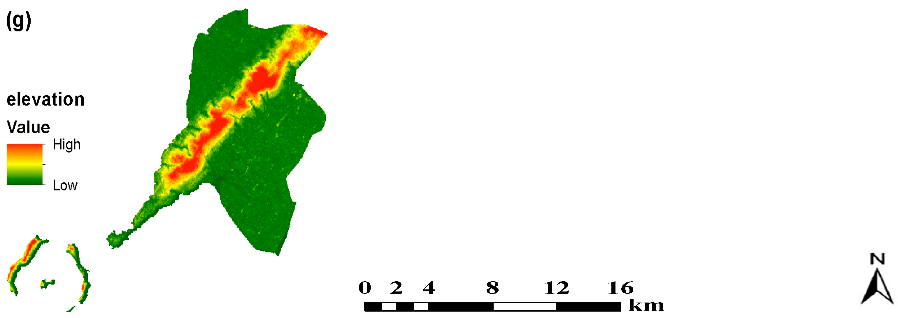
An LRM was established to examine the relationship between urban growth and the various driving forces and to simulate an urban growth probability map for the study area. The LRM results (Table 8) indicated that the socioeconomic proximity variables (distances to urbanized area, to industrial zones, and to major roads) and the topography variables (slope and elevation) were positive and were significantly correlated with the urban growth processes in the study area. These results illustrate that urban growth has been affected by both socioeconomic proximity factors and topography factors. Urban growth in Conakry has been very uneven, with much of the growth concentrated along major roads which are located at high elevation, as can be observed from elevation and major road maps in Figure 7. This finding is also supported by study conducted by the World Bank on accessing urban services and poverty in Conakry [39]. The World Bank found that living far away from major roads greatly reduced the ability of the population to access urban services. The same study also found that the poor population was more vulnerable because they lived on the outskirts of the city and had to travel some distance to reach the major roads. Similar case studies of cities in other developing countries Tripoli (Lybia) and Lagos (Nigeria) have shown that socioeconomic proximity variables and topograhy factors were key drivers of the urban growth process. These results are very similar to our findings in Conakry with small differences in the order of the drivers. Furthermore, Conakry is a coastal city; and has never ceased to attract people. In recent years, urbanization has become quite rapid; however, the potential impact of the hazards is largely driven by the increasing concentration of population and economic activities. Studies have shown that many cities in the world could suffer serious losses due to flooding over the next decades [40]. Therefore, an emphasis on policies of sustainable urban planning and management is urgently needed.
5.3. Weakness of This Study
It is important to recognize that only socioeconomic proximity and topography factors were included in this model, and that the model could be improved by incorporating additional explanatory factors such as demographic (population density) and socioeconomic indicators (income per capita in urban and rural areas, migration). However, due to a lack of available geospatial and socioeconomic data in developing countries such as Guinea, we focused on certain variables. We implemented a robust statistical approach to explicitly examine the relationship between urban growth processes and various drivers, and developed an urban growth probability map for Conakry. The results of this research will not only assist urban planners and policy makers in Conakry, but will also serve as an important reference for future urban sustainability studies in Guinea.
6. Conclusions
The aim of the present study was to integrate GIS and RS techniques with an LRM to analyze and quantify urban growth patterns in the capital of Guinea, Conakry, and to investigate the relationship between urban growth and various explanatory variables. The LULC change results indicated patterns of a degraded and disturbed LULC and a continuous increase in urban land area. This net increase in urban area was likely caused by different anthropogenic activities such as conversion of vegetation cover to urban land cover. Subsequently, LRM was used in modeling and understanding the drivers in the urban growth process and simulate an urban growth probability map that showed likely areas of urban. The results have shown that the proximity variable, distance to major roadsand the topography variable, elevation had the highest coefficients and resulted in the model with the best fit, which impling a high probability of urban growth areas with high elevation and near major roads.
Acknowledgments
The Ministry of Education, Culture, Sports, Science and Technology of Japan (MEXT) supported this study for the promotion of science.
Author Contributions
Arafan Traore conducted the fieldwork, analyzed the datasets, Arafan Traore and Teiji Watanabe wrote the first draft of the manuscript, and addressed the reviewers’ comments.
Conflicts of Interest
The authors declare no conflict of interest.
References
- United Nations. World Urbanization Prospects 2014: Highlights; United Nations Environment Programme; United Nations: New York, NY, USA, 2014. [Google Scholar]
- Linard, C.; Tatem, A.J.; Gilbert, M. Modelling spatial patterns of urban growth in Africa. Appl. Geogr. 2013, 44, 23–32. [Google Scholar] [CrossRef] [PubMed]
- Pickett, S.T.A.; Cadenasso, M.L.; Grove, J.M.; Boone, C.G.; Groffman, P.M.; Irwin, E.; Kaushal, S.S.; Marshall, V.; McGrath, B.P.; Nilon, C.H.; et al. Urban ecological systems: Scientific foundations and a decade of progress. J. Environ. Manag. 2011, 92, 331–362. [Google Scholar] [CrossRef] [PubMed]
- Aguayo, M.; Wiegand, T.; Azócar, G.; Wiegand, K.; Vega, C. Revealing the Driving Forces of Mid-Cities Urban Growth Patterns Using Spatial Modeling: A Case Study of Los Ángeles, Chile. Ecol. Soc. 2007, 12. Article 13. [Google Scholar] [CrossRef]
- Goerg, O. Conakry. Capital Cities in Africa Power Powerlessness. 2011. Available online: http://www.codesria.org/spip.php?article1603 (accessed on 7 March 2017).
- Jasse, A. Image of the Day. Available online: https://earthobservatory.nasa.gov (accessed on 7 April 2017).
- Sylla, L.; Xiong, D.; Zhang, H.Y.; Bangoura, S.T. A GIS technology and method to assess environmental problems from land use/cover changes: Conakry, Coyah and Dubreka region case study. Egypt. J. Remote Sens. Space Sci. 2012, 15, 31–38. [Google Scholar] [CrossRef]
- The World Bank. Guinea—Conakry Urban Development Project; The World Bank: Washington, DC, USA, 1984. [Google Scholar]
- Lagarias, A. Urban sprawl simulation linking macro-scale processes to micro-dynamics through cellular automata, an application in Thessaloniki, Greece. Appl. Geogr. 2012, 34, 146–160. [Google Scholar] [CrossRef]
- Yue, W.; Liu, Y.; Fan, P. Measuring urban sprawl and its drivers in large Chinese cities: The case of Hangzhou. Land Use Policy 2013, 31, 358–370. [Google Scholar] [CrossRef]
- Yusuf, A.Y.; Biswajeet, P.; Mohammed, O.I. Spatio-temporal Assessment of Urban Heat Island Effects in Kuala Lumpur Metropolitan City Using Landsat Images. J. Indian Soc. Remote Sens. 2014, 42, 829–837. [Google Scholar] [CrossRef]
- Triantakonstantis, D. Urban growth prediction: A review of computational models and human perceptions. J. Geogr. Inf. Syst. 2012, 4, 555–587. [Google Scholar] [CrossRef]
- Gao, J.; Li, S. Detecting spatially non-stationary and scale-dependent relationships between urban landscape fragmentation and related factors using Geographically Weighted Regression. Appl. Geogr. 2011, 31, 292–302. [Google Scholar] [CrossRef]
- Luo, J.; Wei, Y.H.D. Modeling spatial variations of urban growth patterns in Chinese cities: The case of Nanjing. Landsc. Urban Plan. 2009, 91, 51–64. [Google Scholar] [CrossRef]
- Jokar Arsanjani, J.; Helbich, M.; Kainz, W.; Darvishi Boloorani, A. Integration of logistic regression, Markov chain and cellular automata models to simulate urban expansion. Int. J. Appl. Earth Obs. Geoinf. 2013, 21, 265–275. [Google Scholar] [CrossRef]
- Pradhan, B. Flood susceptible mapping and risk area delineation using logistic regression, GIS and remote sensing. J. Spat. Hydrol. 2009, 9, 1–18. [Google Scholar]
- Aly, B.C.; Malick, S. Infrastructures Urbaines 1. 2012. Available online: http://www.disonslaveriteguinee.net/wp-content/uploads/2014/01/french_-_infrastructures_urbaines.pdf (accessed on 7 April 2017).
- Audits Urban, Oganisationnel et Financier de la Ville et des Communes de Conakry; Tunis, 2007. Available online: http://documents.worldbank.org/curated/en/274401468035962158/pdf/33541.pdf (accessed on 7 April 2017).
- Nong, Y.; Du, Q. Urban growth pattern modeling using logistic regression. Geo-Spat. Inf. Sci. 2011, 14, 62–67. [Google Scholar] [CrossRef]
- Sweet, S.A.; Grace-Martin, K.A. Data Analysis with SPSS: A First Course in Applied Statistics, 4th ed. Available online: https://www.pearsonhighered.com/program/Sweet-Data-Analysis-with-SPSS-A-First-Course-in-Applied-Statistics-4th-Edition/PGM334221.html (accessed on 7 January 2017).
- Kleinbaum, D.G.; Klein, M. Logistic Regression: A Self-Learning Text Statistics for Biology and Health, 3rd ed.; Springer: New York, NY, USA, 2010. [Google Scholar]
- Huang, B.; Zhang, L.; Wu, B. Spatiotemporal analysis of rural–urban land conversion. Int. J. Geogr. Inf. Sci. 2009, 23, 379–398. [Google Scholar] [CrossRef]
- Mahiny, A.S.; Turner, B.J. Modeling Past Vegetation Change through Remote Sensing and GIS: A Comparison of Neural Networks and Logistic Regression Methods. In Proceedings of the 7th International Conference on Geocomputation, University of Southampton, Southampton, UK, 8–10 September 2003. [Google Scholar]
- Lin, Y.P.; Chu, H.J.; Wu, C.F.; Verburg, P.H. Predictive Ability of Logistic Regression, Auto-Logistic Regression and Neural Network Models in Empirical Land-Use Change Modeling—A case study. Int. J. Geogr. Inf. Sci. 2011, 25, 65–87. [Google Scholar] [CrossRef]
- Eyoh, A.; Olayinka, N.; Nwilo, P.; Okwuashi, O.; Isong, M.; Udoudo, D. Modelling and Predicting Future Urban Expansion of Lagos, Nigeria from Remote Sensing Data Using Logistic Regression and GIS. Int. J. Appl. Sci. Technol. 2012, 2, 116–124. [Google Scholar]
- Parks, J.J.; Champagne, A.R.; Costi, T.A.; Shum, W.W.; Pasupathy, A.N.; Neuscamman, E.; Flores-Torres, S.; Cornaglia, P.S.; Aligia, A.A.; Balseiro, C.A.; et al. Mechanical control of spin states in spin-1 molecules and the underscreened Kondo effect. Science 2010, 328, 1370–1373. [Google Scholar] [CrossRef] [PubMed]
- Akinwande, M.O.; Dikko, H.G.; Samson, A. Variance Inflation Factor: As a Condition for the Inclusion of Suppressor Variable(s) in Regression Analysis. Open J. Stat. 2015, 5, 754–767. [Google Scholar] [CrossRef]
- Midi, H.; Sarkar, S.K.; Rana, S. Collinearity diagnostics of binary logistic regression model. J. Interdiscip. Math. 2010, 13, 253–267. [Google Scholar] [CrossRef]
- Menard, S. Six approaches to calculating standardized logistic regression coefficients. Am. Stat. 2004, 58, 218–223. [Google Scholar] [CrossRef]
- Alsharif, A.A.A.; Pradhan, B. Urban Sprawl Analysis of Tripoli Metropolitan City (Libya) Using Remote Sensing Data and Multivariate Logistic Regression Model. J. Indian Soc. Remote Sens. 2014, 42, 149–163. [Google Scholar] [CrossRef]
- Eastman, J.R. IDRISI Selva Tutorial. Man. Version 17. 2012. Available online: http://uhulag.mendelu.cz/files/pagesdata/eng/gis/idrisi_selva_tutorial.pdf (accessed on 15 January 2017).
- Pontius., R.G., Jr.; Batchu, K. Using the Relative Operating Characteristic to Quantify Certainty in Prediction of Location of Land Cover Change in India. Trans. GIS 2003, 7, 467–484. [Google Scholar] [CrossRef]
- Pontius, R.G.; Schneider, L.C. Land-cover change model validation by an ROC method for the Ipswich watershed, Massachusetts, USA. Agric. Ecosyst. Environ. 2001, 85, 239–248. [Google Scholar] [CrossRef]
- Ayalew, L.; Yamagishi, H. The application of GIS-based logistic regression for landslide susceptibility mapping in the Kakuda-Yahiko Mountains, Central Japan. Geomorphology 2005, 65, 15–31. [Google Scholar] [CrossRef]
- Hosmer, D.W.; Hosmer, T.; le Cessie, S.; Lemeshow, S. A comparison of goodness-of-fit tests for the logistic regression model. Stat. Med. 1997, 16, 965–980. [Google Scholar] [CrossRef]
- Menard, S. Quantitative Applications in the Social Sciences, 2nd ed.; SAGE Publication, Inc.: Thousand Oaks, CA, USA, 1995; Volume 106. [Google Scholar]
- Clark, W.; Hosking, P. Statistical Methods for Geographers; Wiley: New York, NY, USA, 1986. [Google Scholar]
- Hensher, D.A.; Johnson, L.W. Applied Discrete Choice Modelling. 1981. Available online: https://trid.trb.org/view.aspx?id=1206392 (accessed on 23 August 2016).
- World Bank. Poverty and Urban Mobility in Conakry. Available online: http://www.gtkp.com/assets/uploads/20091127-171237-6675-Conakry_en.pdf (accessed on 3 October 2016).
- UNU-IDHP Coastal Zones and Urbanization: Summary for Decision-Makers. Available online: http://www.futureearth.org/sites/default/files/files/IHDP%20SDM%20costalzones_and_urbanization-1.pdf (accessed on 3 November 2016).
Figure 1.
Location of Conakry in Guinea.

Figure 2.
Dependent variable (Y): (a) urban growth 1986–2000; and (b) urban growth 2000–2016.
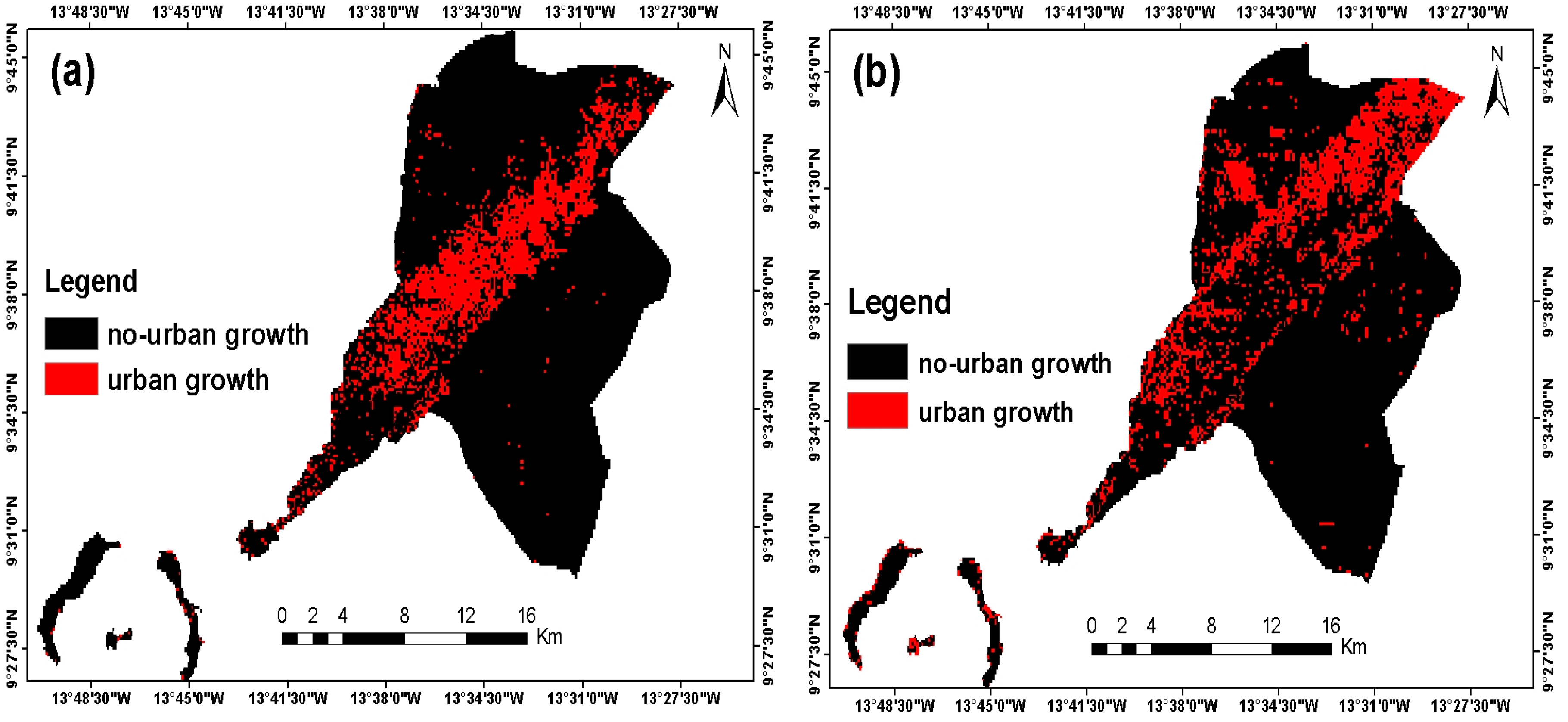
Figure 3.
Relative operating characteristics curve.

Figure 4.
LULC change maps of Conakry in (a) 1986, (b) 2000 and (c) 2016.

Figure 5.
Changing pattern in LULC over in the study area.
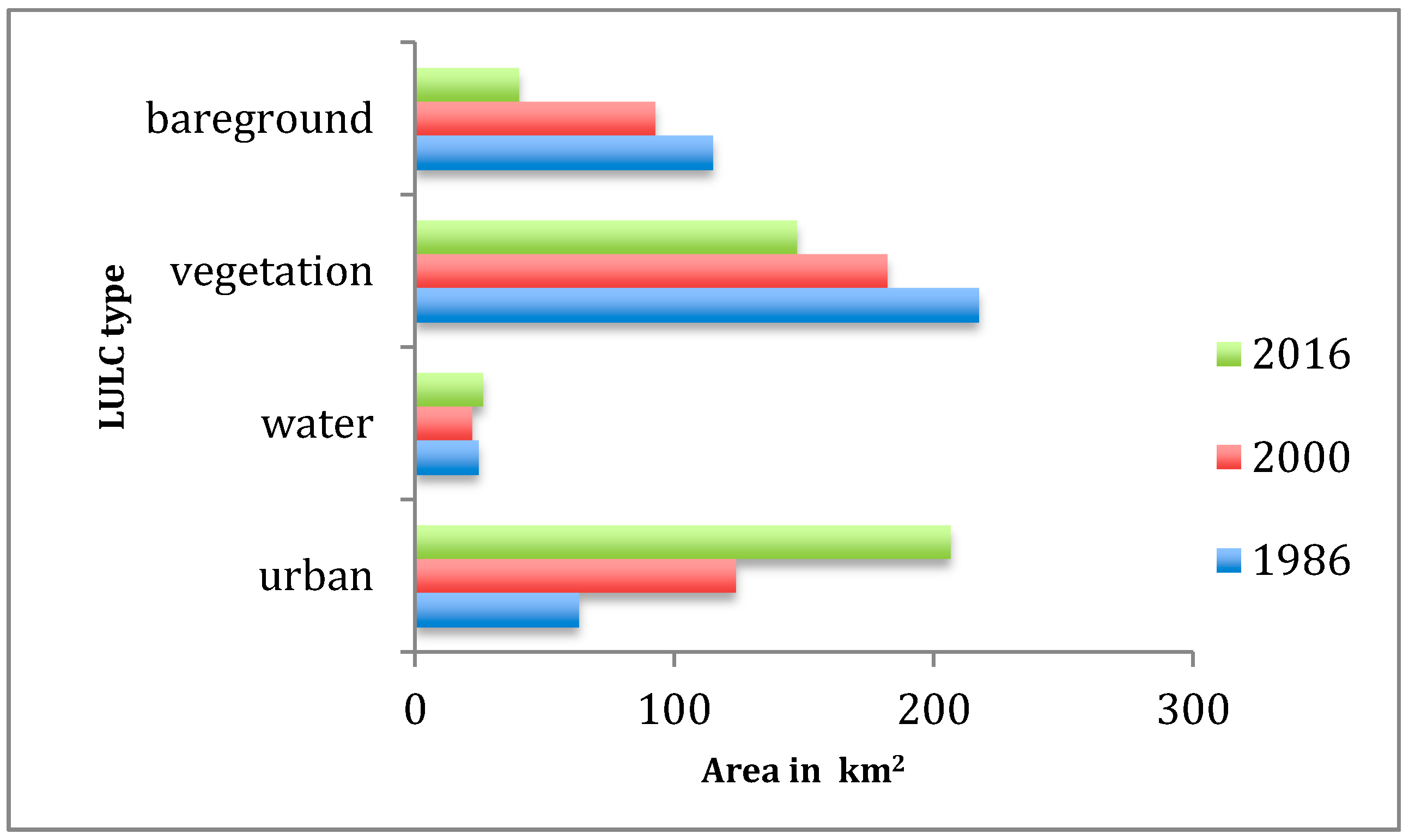
Figure 6.
Urban growth probability map for 2016.
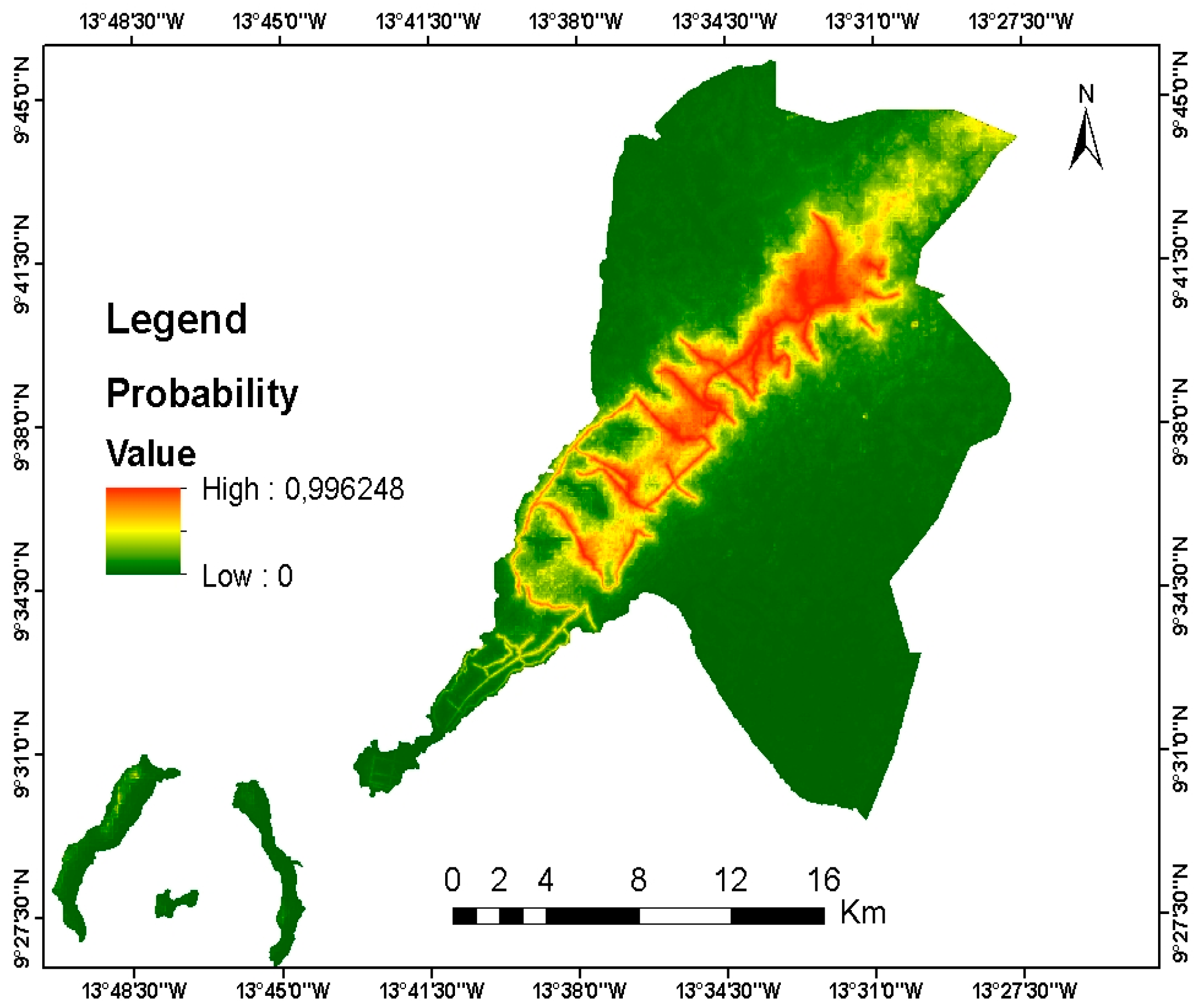
Figure 7.
Raster images of the explanatory variables included in the LRM (a) distance to the active economic center (DAEC), (b) distance to urbanized areas (DUR), (c) distance to industrial zones (DIZ), (d) distance to major roads (DMR), (e) distance to the international airport (DIA), (f) slope, and (g) elevation.


Table 1.
Data used and their sources.
| Data | Data Source |
|---|---|
| Landsat (TM 1986) | USGS Earth Explorer |
| Landsat (ETM +2000) | USGS Earth Explorer |
| Landsat (OLI 2016) | USGS Earth explorer |
| Administrative boundary map | Diva-GIS |
| Aster DEM | USGS Earth Explorer |
| Roads Network | Diva-GIS |
| Active Economic Center | Google Earth, digitized |
| International Airport | Google Earth digitized |
| Industrial | Open Street Map downloaded |
| Ground controll point data | Garmin GPS |
Table 2.
List of the explanatory variables included in the model.
| Variable | Description | Nature |
|---|---|---|
| Dependent (Y) | 1 Urban growth, 0 no urban growth | Dummy |
| Explanatory variable | ||
| Socioeconomic factors | ||
| DAEC | Distance to active economic center | Continuous |
| DUA | Distance to urbanized areas | Continuous |
| DIZ | Distance to industrial zones | Continuous |
| DMR | Distance to major roads | Continuous |
| DIA | Distance to international airport | Continuous |
| Topography factors | ||
| Slope | Percentage rise | Continuous |
| Elevation | Elevation | Continuous |
Table 3.
Correlation Coefficients and the Variance Inflation Factors (VIF) of the explanatory variables.
Table 3.
Correlation Coefficients and the Variance Inflation Factors (VIF) of the explanatory variables.
| Variable | DAEC | DUA | DIZ | DMR | DIA | Slope | Elevation | VIF |
|---|---|---|---|---|---|---|---|---|
| DAEC | 1 | 0.029 | 0.44 | 0.31 | 0.30 | 0.09 | 0.13 | 1.99 |
| DUA | 1 | 0.58 | 0.53 | 0.50 | −0.48 | −0.46 | 1.62 | |
| DIZ | 1 | 0.75 | 0.51 | −0.32 | −0.41 | 7.84 | ||
| DMR | 1 | 0.58 | −0.43 | −0.54 | 5.86 | |||
| DIA | 1 | −0.24 | −0.26 | 3.20 | ||||
| Slope | 1 | 0.58 | 1.21 | |||||
| Elevation | 1 | 1.17 |
Table 4.
Association between dependent variable and explanatory variables using Cramer’s (V).
| Explanatory Variables | Cramer’s V | p Value |
|---|---|---|
| DAEC | 0.15 | 0.00 |
| DUA | 0.22 | 0.00 |
| DIZ | 0.32 | 0.00 |
| DMR | 0.39 | 0.00 |
| DIA | 0.22 | 0.00 |
| Slope | 0.32 | 0.00 |
| Elevation | 0.42 | 0.00 |
Table 5.
Two by two contingency table showing the number of grid cells in actual map versus a predicted map.
Table 5.
Two by two contingency table showing the number of grid cells in actual map versus a predicted map.
| Actual Map | Total | |||
|---|---|---|---|---|
| Urban Growth (1) | No-Urban Growth (0) | |||
| Predicted Image | Urban growth (1) | A | B | A+B |
| No-urban growth (0) | C | D | C+D | |
| Total | A + C = 95,941 | B + D = 1,613,435 | A + B + C + D = 1,709,376 | |
Table 6.
LULC area changes over the study periods.
| Year | 1986 | 2000 | 2016 | |||
|---|---|---|---|---|---|---|
| LULC | Area (km2) | Area (%) | Area (km2) | Area (%) | Area (km2) | Area (%) |
| urban | 63.03 | 0.15 | 123.76 | 0.29 | 206.58 | 0.49 |
| water | 24.63 | 0.05 | 21.80 | 0.05 | 26.10 | 0.06 |
| vegetation | 217.48 | 0.51 | 181.86 | 0.43 | 147.32 | 0.35 |
| bare ground | 114.76 | 0.27 | 92.49 | 0.22 | 39.88 | 0.09 |
| Total | 419.90 | 1.00 | 419.90 | 1.00 | 419.90 | 1.00 |
Table 7.
Coefficients of the 7 explanatory variables used in the logistic regression.
| Variable | Coefficient | |
|---|---|---|
| Intercept | 7.03 | |
| DAEC | −0.01 | |
| DUA | 0.39 | |
| DIZ | 0.02 | |
| DMR | 0.67 | |
| DIA | −0.06 | |
| Slope | 0.27 | |
| Elevation | 1.76 | |
Table 8.
Statistics for the 7 explanatory variables.
| Number of Total Observation | 1,709,376 |
|---|---|
| Number of 0 | 1,619,469 |
| Number of 1 | 89,907 |
| −2logLo | 67,290.6403 |
| −2log(likelihood) | 32,635.0373 |
| pseudo R2 | 0.5150 |
| Goodness of Fit | 202,668.3024 |
| Chi-Square(7) | 34,655.6030 |
| ROC | 0.96 |
© 2017 by the authors. Licensee MDPI, Basel, Switzerland. This article is an open access article distributed under the terms and conditions of the Creative Commons Attribution (CC BY) license (http://creativecommons.org/licenses/by/4.0/).
Share and Cite
MDPI and ACS Style
Traore, A.; Watanabe, T. Modeling Determinants of Urban Growth in Conakry, Guinea: A Spatial Logistic Approach. Urban Sci. 2017, 1, 12. https://doi.org/10.3390/urbansci1020012
AMA Style
Traore A, Watanabe T. Modeling Determinants of Urban Growth in Conakry, Guinea: A Spatial Logistic Approach. Urban Science. 2017; 1(2):12. https://doi.org/10.3390/urbansci1020012
Chicago/Turabian StyleTraore, Arafan, and Teiji Watanabe. 2017. "Modeling Determinants of Urban Growth in Conakry, Guinea: A Spatial Logistic Approach" Urban Science 1, no. 2: 12. https://doi.org/10.3390/urbansci1020012