Linear Stability Prediction of Vortex Structures on High Pressure Turbine Blades  ^†

Abstract

Velocity profiles are extracted from time- and span-averaged direct numerical simulation data, describing the flow over a high-pressure turbine vane linear cascade near engine-scale conditions with reduced inlet disturbance levels. Based on these velocity profiles, local as well as non-local linear stability analysis of the boundary-layer over the suction side of the vane is carried out in order to characterise a linearly unstable region close to the trailing edge. The largest growth rates are found for oblique modes, but those are only slightly more unstable than 2D modes, which describe the locations and frequencies of most unstable modes very well. The frequencies of the most unstable linear modes predict with good accuracy the predominant frequencies found in the direct numerical simulations (DNS) close to the trailing edge.

1. Introduction

In order to design more efficient high-performance turbines, an improved understanding and prediction of laminar-turbulent boundary-layer (BL) transition is crucial. As computational resources and the performance of solution algorithms are increasing, direct numerical simulations (DNS) are becoming more and more feasible even for complex flowfields, such as high-pressure turbines (HPT). In order to maintain a laminar BL for loss reduction, it is important to identify the characteristics of naturally unstable disturbances and reduce the excitation of these modes. Furthermore, the prediction of laminar-turbulent transition is of particular interest. The authors of [1] performed a computationally costly transient growth analysis of the flow over an array of low-pressure turbine blades, however the Reynolds numbers were limited to relatively low values of 2000. As BL phenomena are highly resolved in DNS, a reassessment of less expensive and powerful stability methods involving linear stability theory (LST) or linear parabolised stability equations (LPSE) is possible. The results of the analysis improve understanding of the origin and development of vortex structures occurring in the BL and triggering the final breakdown to turbulence. Disturbance growth rates help to improve empirical laws for predicting transition and can also provide characteristic length- and time-scales for turbulence models that are used in design studies. The output of such methods can also be used to study active or passive flow control, since the computational effort is low compared to DNS. Additionally, LST can be applied to evaluate the spanwise domain width of three-dimensional (3D) simulations regarding the ability to capture oblique linearly unstable waves.

2. Direct Numerical Simulation (DNS)

The non-dimensional, fully compressible 3D Navier Stokes Equations (NSE) are solved using an in-house multi-block structured compressible Navier-Stokes solver, called HiPSTAR. For the time integration, a five-step, fourth-order accurate low-storage Runge-Kutta method is used and for the spatial discretisation in the streamwise and pitchwise directions, a wavenumber-optimised compact finite-difference scheme is applied. The discretisation in the spanwise direction was done by applying a Fourier method using the FFTW3 library. More details regarding the DNS methodology are provided by [2,3].

Using this approach, Wheeler et al. [2] performed a fully resolved DNS for an HPT vane with a Reynolds number of 570,000 and a Mach number of $0.9$ (both at reference conditions at the vane exit). The inlet turbulence intensity was set to $3.5\%$. A structured grid, consisting of 645 million grid-points was used for a spanwise domain width of $10\%$ of the axial chord, which means that 2D modes with a spanwise wavenumber of zero and oblique modes with spanwise wavenumbers greater than ${\beta }_r=62$ can be captured. In order to extract a base flow for linear stability analysis, Favre-averaging of the flow quantities was applied, considering a time window of four flow-through times. Finally, the flowfield was also averaged in the spanwise direction.

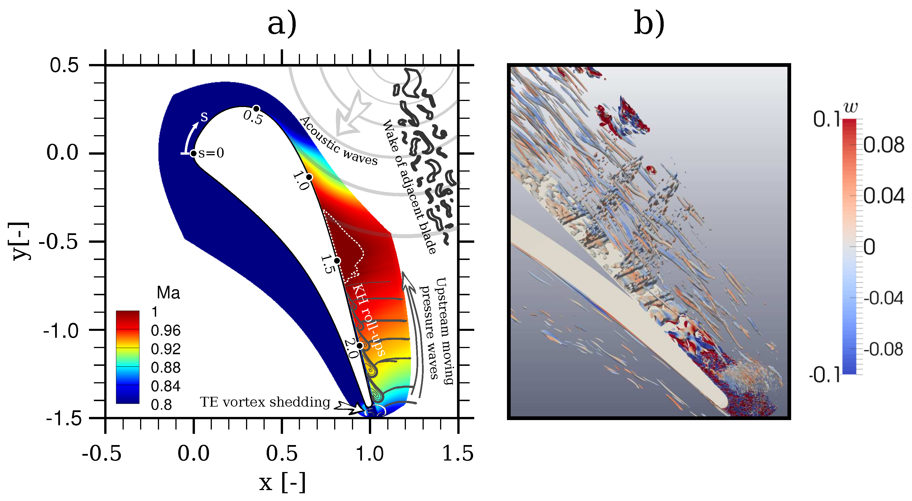
For the DNS, the coordinates are defined as x and y in directions parallel and normal to the inlet velocity vector respectively, while z represents the spanwise coordinate. The origin is located at the leading edge. To perform a linear stability analysis, wall-normal velocity-profiles are extracted from the DNS data, corresponding to a coordinate transformation. The first coordinate for identifying the position of the velocity profiles is denoted by the surface-distance (s), which describes the distance from the leading edge along the surface to each point on the suction side of the blade. The second coordinate n denotes the wall-distance. A Cartesian domain for the BL is obtained, where the abscissa ($n=0$) represents the suction surface of the HPT vane.

Figure 1a shows the Mach number of the time- and span-averaged flowfield of the HPT simulation and is annotated with sketches of observed flow-phenomena and potential disturbance sources that might excite linearly unstable modes. A notable feature is the upstream-travelling waves originating from the trailing edge (TE), which appears to interact with Kelvin Helmholtz (KH) instabilities. An instantaneous snapshot in Figure 1b shows vortex structures and a breakdown into turbulence in the area of interest near the TE, where the main linear instabilities are expected [2].

Wall-normal velocity profiles are extracted and interpolated onto a Chebychev grid. The resolution, denoted by the number of Chebychev-Gauss-Lobatto collocation points, has to be sufficiently high to get grid-independent results. In order to increase the numerical robustness, all profiles are carefully smoothed in the wall-normal direction without changing the main characteristics. The resulting smoothed profiles using 200 Chebychev-Gauss-Lobatto collocation points show good agreement with a set of raw profiles represented by 1600 collocation points. The smoothed base flow is preferred to the raw data, as the wall-normal profiles are smooth up to the second derivatives of velocity, density and pressure. In order to obtain consistent and stable results applying the non-local LPSE approach, all velocity profiles are interpolated onto a numerical grid (uniform in the s-direction) and smoothed in the s-direction along the suction-side surface. The smoothing in the s-direction has hardly any impact on the LST-results, but leads to stable LPSE results for an integration step size of $\Delta s_{PSD}=0.0234$ in the linearly unstable region. The results regarding a sensitivity analysis of the base flow are summarised in

Table 1. Summary of temporal linear stability theory (LST) results using different base flows and numbers of Chebychev-Gauss-Lobatto collocation points. The first two columns indicate whether a filter is applied in the wall-normal (n) or wall-tangential (s) direction. The third column denotes the number of Chebychev-Gauss-Lobatto collocation points. Columns four to six represent the streamwise wavenumber ${\alpha }_r$, the spanwise wavenumber ${\beta }_r$ and the surface-distance s, while the last three columns show the LST-output consisting of the angular frequency ${\omega }_r$, the growth rate ${\omega }_i$ and the phase speed $c_{ph}$.

Smooth-n	Smooth-s	Cheb. Grid	${\mathit{\alpha }}_{\mathit{r}}$	${\mathit{\beta }}_{\mathit{r}}$	s	${\mathit{\omega }}_{\mathit{r}}$	${\mathit{\omega }}_{\mathit{i}}$	${\mathit{c}}_{\mathit{ph}}$
NO	NO	1600	80	0	1.96	178.667	38.475	2.233
YES	NO	1600	80	0	1.96	178.667	38.476	2.233
YES	NO	200	80	0	1.96	178.608	38.374	2.233
YES	YES	200	80	0	1.96	178.585	38.380	2.232

for a representative position at $s=1.9637$. For the stability analysis discussed in this work, the generated velocity profiles consist of 300 data points, which are extracted from the DNS-data and smoothed. To resolve the profile, 200 Chebychev collocation points are used.

3. Linear Stability Theory and Parabolised Stability Equations

The basis for the LST is provided by the Orr-Sommerfeld equation (OSE), which is derived from the compressible NSE considering a 2D flowfield ([4] provides further detail on the derivation of the OSE). The flowfield is decomposed as

$$\begin{array}{cc}\hfill Q& =\overline{q}+q^{\prime },\hfill \end{array}$$

(1)

where $\overline{q}$ represents the steady base flow and $q^{\prime }$ denotes superimposed disturbances. The vector Q contains the dimensionless flow quantities. The perturbations are represented as normal-mode solutions

$$\begin{array}{cc}\hfill q(s,n,z,t)& =\widehat{q}\left(n\right)·e^{i(\alpha s+\beta z-\omega t)},\hfill \end{array}$$

(2)

where $\widehat{q}$ represents the amplitude of the disturbance, while $\alpha$ and $\beta$ are the complex streamwise and spanwise wavenumbers, respectively, and $\omega$ stands for the complex frequency. Neglecting non-linear terms as well results in an eigenvalue-problem corresponding to

$$\begin{array}{cc}\hfill \underline{L}\widehat{q}& =\omega \underline{K}\widehat{q},\hfill \end{array}$$

(3)

where $\underline{L}$ contains only terms including $\alpha$ and $\beta$. For the temporal LST approach, the disturbance of interest has to be defined by the wavenumbers ${\alpha }_r$ and ${\beta }_r$, while the spatial growth rate ${\alpha }_i$ is set to zero. As an output, we get the angular frequency ${\omega }_r$ and the temporal growth rate ${\omega }_i$ of the considered wave. The spatial approach works basically the other way around and provides the spatial growth rate of disturbances with a certain frequency. For the results presented here Sutherland’s law is used to model the viscosity as a function of the temperature, which is consistent with the DNS solver. Gaster [5] describes the correlation between temporally and spatially growing waves for hydrodynamic problems by

$$\begin{array}{c}\hfill \frac{{\omega }_i^T}{{\alpha }_i^S}=-\frac{\partial {\omega }_r}{\partial {\alpha }_r}=-c_g,\end{array}$$

(4)

where $c_g$ is called group velocity and the superscript T denotes results obtained by the temporal approach, while S denotes results obtained by the spatial approach. In [6] , the authors note that the accuracy of that correlation decreases with higher growth-rates, as the transform is only exact for ${\omega }_i\mapsto 0$. As the magnitude of the disturbance-amplitude is not relevant for solving the OSE, the eigenfunctions are normalized, so that the Euclidean norm equals one. For comparison of LST results with actual DNS or test data, the so called N-factors (N) are calculated according to

$$\begin{array}{c}\hfill N=ln\left(\frac{A\left(s\right)}{A\left(s_0\right)}\right)={\int }_{s_0}^s-{\alpha }_i\left(s\right)·ds,\end{array}$$

(5)

where $A\left(s_0\right)$ denotes the initial disturbance-amplitude at $s=s_0$.

As the parallel flow assumption is a significant restriction for our problem, the LPSE are introduced as well. The derivation is similar, but the disturbances are modelled by a different ansatz according to

$$\begin{array}{cc}\hfill q& =\widehat{q}(s,n)·e^{i[{\int }_{s_0}^{s_n}\alpha ds+\beta z-\omega t]}\hfill \end{array}$$

(6)

An eigenvalue problem defined by

$$\begin{array}{cc}\hfill 0& =(\underline{L}+{\underline{L}}_P-\underline{K})\widehat{q}+\underline{M}\frac{\partial \widehat{q}}{\partial s}+\underline{N}\frac{d\alpha }{ds}\widehat{q}\hfill \end{array}$$

(7)

is obtained, where $\underline{L}$ and $\underline{K}$ are the same matrices as before and ${\underline{L}}_P$, $\underline{M}$ and $\underline{N}$ include all non-parallel terms. Assuming only slowly varying flows in the streamwise direction allows further simplification. In order to solve the resulting closure problem, a normalisation condition according to

$$\begin{array}{cc}\hfill 0& ={\int }_0^{\infty }{\widehat{q}}^{†}\frac{\partial \widehat{q}}{\partial s}dn\hfill \end{array}$$

(8)

is applied, where the dagger denotes the complex conjugate of the flow quantities. For the non-parallel problem, the spatial growth rate as well as the streamwise wavenumber have to be corrected as the disturbance also varies in the streamwise direction. Further details regarding the derivations and the in-house code NoSTRANA are provided by [7].

4. Temporal Linear Stability Theory Results

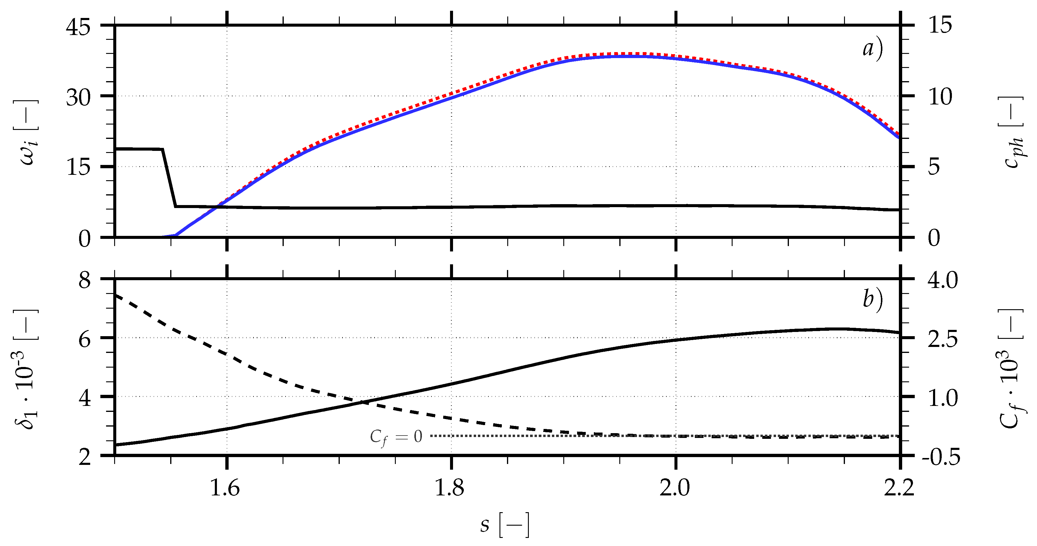
A temporal linear stability analysis is performed for the whole suction surface of the HPT blade. For several positions between $s=0$ and $s=2.33$ (with a step-width of $\Delta s=0.0117$), a sweep was made over the streamwise wavenumber ${\alpha }_r$ (${\alpha }_{r,min}=5$, ${\alpha }_{r,max}=300$ and $\Delta {\alpha }_r=1$), keeping a constant spanwise wavenumber of ${\beta }_r=0$, to get an overview of the most unstable 2D modes. The most unstable region is found to be located near the TE and arises shortly after an inflectional velocity profile appears. The evolution of the temporal growth rate ${\omega }_i$ of the most unstable 2D modes in that region is shown in Figure 2a (solid blue line—corresponding to the left-hand scale). In addition to the growth rates, the phase speed ($c_{ph}$—black line) is plotted, corresponding to the right-hand scale. A slightly unstable region for $s\approx 0.5$, which only reaches a maximum growth rate of ${\omega }_i\approx 1$, is not considered here, as it is followed by a very stable region (${\omega }_i<0$), due to the accelerated flow. Also, the section after $s=2.2$ is not evaluated, as transition has already started at that point and non-linear effects are not negligible anymore. Furthermore, non-parallel effects become important in that area.

As a next step, the growth rates of 2D disturbances are compared to 3D (oblique) disturbances at each location. The most unstable oblique disturbances are represented by the red dotted line in Figure 2a. As the difference between the maximum growth rates of 2D and 3D disturbances is small (about 1.5%), an analysis of 2D modes already gives a good impression of the evolution of unstable regions, streamwise wavenumbers and frequencies. At the very beginning of the unstable region, the modes with the highest growth rates are 2D.

Figure 2b shows the skin-friction coefficient ($C_f$—dashed line corresponding to the right-hand scale) as a function of the surface-distance close to the TE as well as the displacement thickness (${\delta }_1$—solid line corresponding to the left-hand scale), which increases as the inflection point in the velocity profiles moves farther away from the wall. One can see that the flow separates slightly between $s=2$ and $s=2.2$ and the displacement thickness peaks at $s\approx 2.15$, while the temporal growth rate reaches its maximum at $s\approx 1.96$. This is due to the fact that the wall-normal velocity gradient at the inflection point is decreasing, which has a stabilising effect.

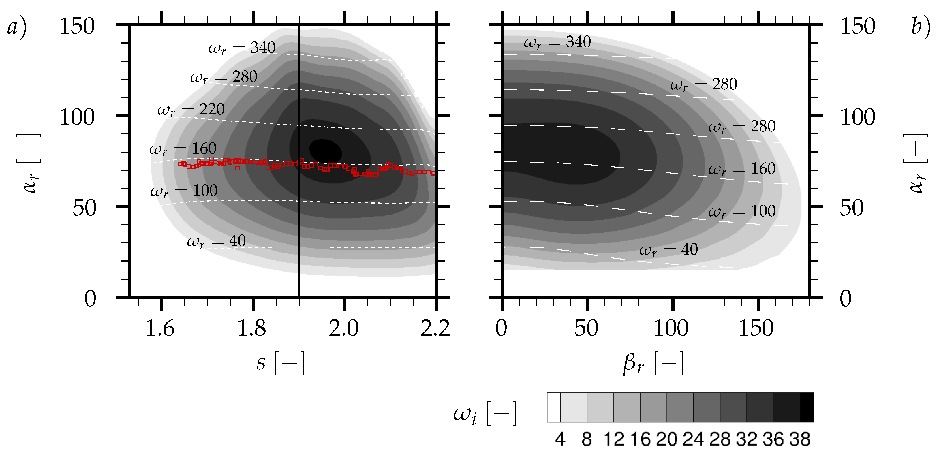
Contours of ${\omega }_i$ for the most unstable 2D modes are shown in Figure 3a as a function of the surface-distance s and the streamwise wavenumber ${\alpha }_r$. The white dashed lines represent corresponding frequencies. It is obvious that the growth rate ${\omega }_i$ of the most unstable modes peaks between $s=1.9$ and $s=2.0$. These modes have a streamwise wavenumber of ${\alpha }_r\approx 80$ and an angular frequency ${\omega }_r$ between 160 and 180. Analysis of the DNS data regarding the surface pressure in that region of the HPT-blade reveals predominant angular frequencies about ${\omega }_r=157$. These angular frequencies were extracted using a time-correlation method and are highlighted in Figure 3a (red symbols □), showing good agreement with the most unstable modes from temporal linear stability analysis. The phase speed of those modes is found to be about 40% of the BL edge velocity, which corresponds as well to the phase speed of instability waves discovered in the DNS-flowfield by [2].

For a representative location on the suction surface ($s=1.9$), Figure 3b illustrates contours of ${\omega }_i$ as a function of streamwise wavenumber ${\alpha }_r$ and spanwise wavenumber ${\beta }_r$. A peak in the growth rates ${\omega }_i$ can be observed around ${\beta }_r\approx 40$. This spanwise wavenumber is lower than the minimum wavenumber of ${\beta }_r=62$ that can be resolved by the DNS discussed here, suggesting that a wider domain would have been needed in the DNS to capture the most unstable linear mode. As the growth rate does not change significantly for low spanwise wavenumbers, the DNS is still expected to have captured the main characteristics of the linear unstable waves and their evolution.

In addition to the temporal approach, a spatial linear stability analysis was conducted for ${\omega }_r=160$. The results are compared with those from the temporal LST, applying the Gaster transform at a very unstable location ($s=1.95$). Details can be found in

Table 2. Summary of LST results for a streamwise wavenumber ${\alpha }_r=73.63$ and spanwise wavenumber ${\beta }_r=0$ at the position $s=1.95$. The table shows the corresponding angular frequencies ${\omega }_r$, temporal growth rates ${\omega }_i^T$, spatial growth rates ${\alpha }_i^S$, phase speeds $c_{ph}$ and group velocities $c_g$ from spatial as well as temporal LST results.

Approach	${\mathit{\alpha }}_{\mathit{r}}$	${\mathit{\omega }}_{\mathit{r}}$	${\mathit{\omega }}_{\mathit{i}}^{\mathit{T}}$	${\mathit{\alpha }}_{\mathit{i}}^{\mathit{S}}$	${\mathit{c}}_{\mathit{ph}}$	${\mathit{c}}_{\mathit{g}}$
Spatial	73.63	160.0	-	−13.436	2.173	2.926
Temporal	73.63	159.3	37.999	−12.991	2.164	2.926

, where the first and second lines show the results of the spatial and temporal LST approach, respectively. The temporal approach used the same streamwise wavenumber ${\alpha }_r$ as given by the spatial approach. The group velocity $c_g$ is calculated based on two temporal results with slightly different ${\omega }_r$. That allows us to calculate a spatial growth rate for the temporal approach, using Equation (4). As the error of the calculated ${\alpha }_i$ based on temporal results is about 3.3%, the Gaster transform can be applied here even for very unstable modes.

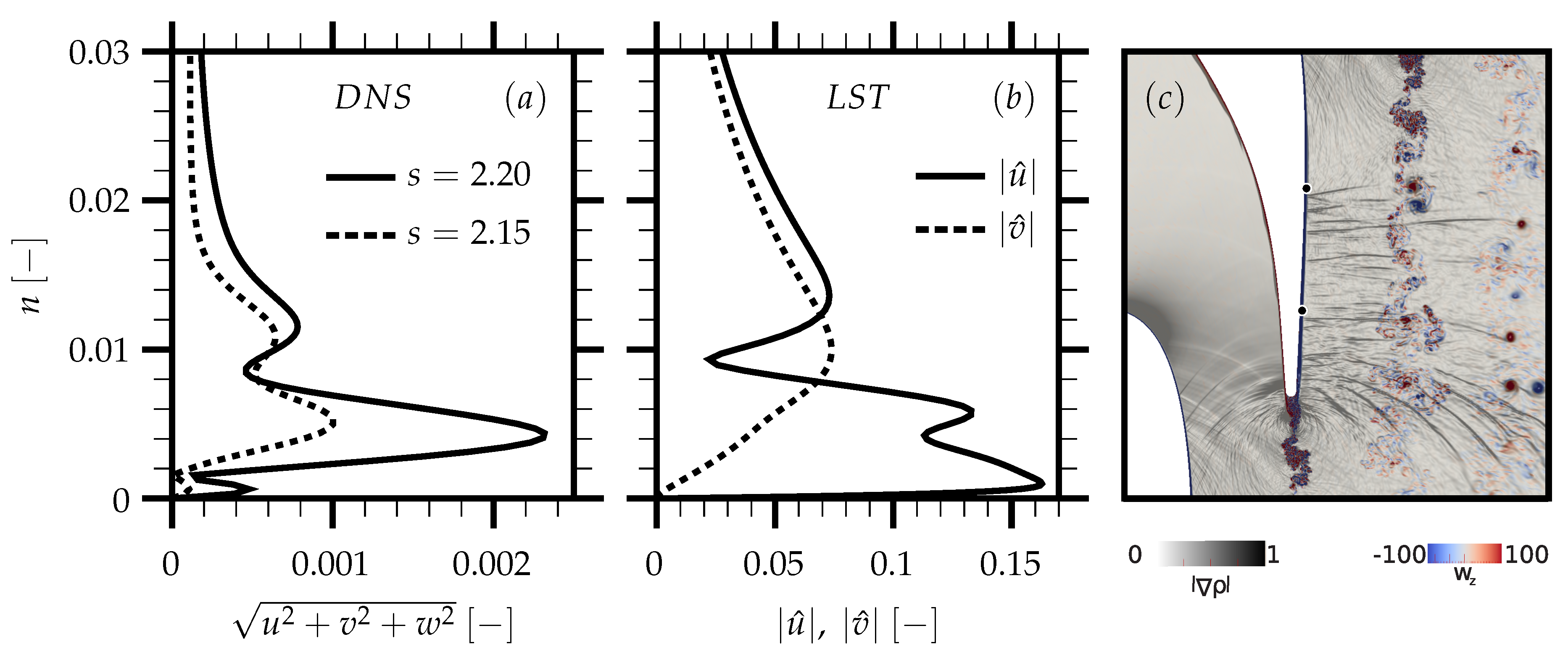
Figure 4a shows the wall-normal profile of the time-averaged magnitude of the fluctuations at two linearly unstable positions ($s=2.15$ and $s=2.2$), which are extracted from the DNS data. Figure 4b shows the eigenfunctions of the disturbances given by a temporal linear stability analysis at $s=2.2$. It is hard to compare both profiles directly, as the DNS profiles contain a whole spectrum of disturbances, background noise and the influence of phenomena like upstream-travelling pressure waves. This complex environment can be seen in Figure 1c as well, showing the phenomena sketched in Figure 1a. Nevertheless, one can see that the disturbances are strongest within a region where the LST suggests that the disturbance-amplitudes are peaking.

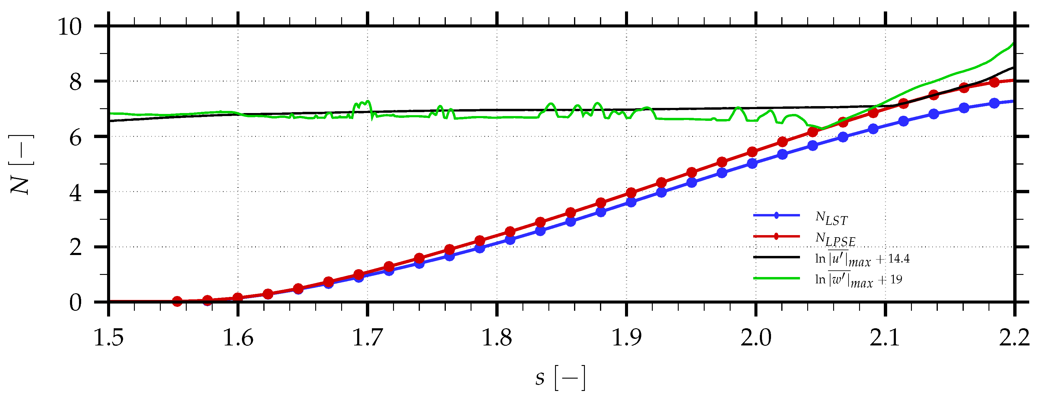
The LPSE are solved for the angular frequency ${\omega }_r=160$ and a downstream-marching integration step size of $\Delta s_{PSE}=0.0234$. A spatial LST solution provides the initial condition. These results are in principle more trustworthy than the LST results, since they account for non-parallel effects. One can clearly see by means of the N-factors in Figure 5 that the spatial LST (blue dots) tends to underestimate the growth rates, resulting in up to 7.6% lower N-factors than these obtained by solving the LPSE (red dots). A similar tendency was also found in [7]. Nevertheless, both approaches show a good correlation, justifying again the use of the more robust LST methodology for the linearly unstable regions of the BL. The good agreement between LST and LPSE indicates a relatively minor influence of non-parallel flow effects in the investigated region.

Wall-normal fluctuation profiles were extracted from the time-averaged DNS data. The black and green lines in Figure 5 represent the logarithm of the maximum values found in those profiles regarding the fluctuation components in the streamwise ($\overline{|u^{\prime }|}$) and spanwise ($\overline{|w^{\prime }|}$) directions as a function of the surface-distance respectively. Both of these lines show a section with hardly changing disturbance amplitudes where the LST and LPSE already suggest the onset of linear growth. As the fluctuation profiles are composed of a whole spectrum of disturbances, the background noise does not allow us to detect the onset of linear instabilities in the time-averaged DNS-data. The jitter in the spanwise disturbances is probably caused by upstream-travelling pressure waves. However, after $s=2.05$ a section of roughly linear growth can be observed in the streamwise as well as spanwise disturbance profiles before non-linear effects start increasing from $s=2.1$ onwards. An offset was applied to the logarithmic disturbance-values in order to match the starting point of the linear growth-section with suggested N-factors from the LPSE approach. The linear section of the streamwise fluctuations from the DNS data corresponds reasonably well with the LPSE results. Even though it is difficult to compare the LPSE (for one mode) with the time-averaged DNS data-set, it appears that linear modes play an important role in the growth-mechanism of disturbances close to the trailing edge.

In combination with trailing edge vortex shedding, which has similar frequencies, there exists the possibility of a feedback mechanism that could support a global mode, but this is a topic for further investigations.

5. Conclusions

Temporal linear stability analysis of BL profiles, extracted from DNS of flow over a linear HPT vane cascade, reveals a dominant unstable section close to the TE. The temporal LST results are cross-checked with those obtained from a spatial LST approach. Applying the Gaster transform, good agreement is found between the two approaches (the difference between growth rates is about 3.3%), even for highly unstable regions. LPSE for a representative frequency also shows good agreement with the LST results, indicating small non-parallel effects in the analysed region. Finally, these unstable linear modes are shown to correspond to time scales found in DNS data close to the TE. Due to an interaction between the vortex shedding at the TE, upstream-moving pressure waves and KH instabilities near the TE, further investigations are needed into the feedback mechanism. The reasonably good correlation between the LPSE results and the growth of disturbance-profiles extracted from time-averaged DNS data supports the assumption of linear instabilities playing a major role in the growth-mechanism of vortex structures close to the trailing edge.

A comparison between the growth rates of 2D and oblique modes, obtained by temporal linear stability analysis, suggests that the streamwise wavenumbers, the frequencies and the locations of the most unstable modes are already well described when only considering 2D disturbances. As the spanwise extent of the DNS is 10% of the axial chord length, the domain is not quite wide enough to capture the mode with spanwise wavenumber ${\beta }_r\approx 40$, which corresponds to the most unstable mode that is suggested by the LST approach. However, the DNS still captures the essential features of 3D breakdown to turbulence within the computational domain and instability growth rates are not very sensitive to ${\beta }_r$ in this range. The temporal LST approach considering only 2D modes is very stable and reveals reasonable frequencies and growth rates of unstable modes. The comparably low computational efforts and the possibility for extensive parallelisation enable coupling with Reynolds-averaged Navier Stokes solvers or other applications.