
A CFD-Based Throughflow Method with Three-Dimensional Flow Features Modelling †


Department of Industrial Engineering, University of Florence, via S. Marta, 3-50139 Florence, Italy
*
Author to whom correspondence should be addressed.
†
This paper is an extended version of our paper in Proceedings of the European Turbomachinery Conference ETC12, 2017, Paper No. 329.
Int. J. Turbomach. Propuls. Power 2017, 2(3), 11; https://doi.org/10.3390/ijtpp2030011
Submission received: 29 March 2017
/
Revised: 16 June 2017
/
Accepted: 16 June 2017
/
Published: 24 June 2017
Abstract
:The paper describes the development and validation of a novel computational fluid dynamics (CFD)-based throughflow model. It is based on the axisymmetric Euler equations with tangential blockage and body forces and inherits its numerical scheme from a state-of-the-art CFD solver (TRAF code). Secondary and tip leakage flow features are modelled in terms of Lamb–Oseen vortices and a body force field. Source and sink terms in the governing equations are employed to model tip leakage flow effects. A realistic distribution of entropy in the meridional and spanwise directions is proposed in order to compute dissipative forces on the basis of a distributed loss model. The applications are mainly focused on turbine configurations. First, a validation of the secondary flow modelling is carried out by analyzing a linear cascade based on the T106 blade section. Then, the throughflow procedure is used to analyze the transonic CT3 turbine stage studied in the framework of the TATEF2 (Turbine Aero-Thermal External Flows) European program. The performance of the method is evaluated by comparing predicted operating characteristics and spanwise distributions of flow quantities with experimental data.
1. Introduction
The design process of multistage turbomachinery is based on the efficient use of the currently available tools, such as one-dimensional meanline models, 2D or quasi-3D blade-to-blade, throughflow and 3D viscous, steady, and unsteady analyses. Throughflow methods traditionally represent a key tool for turbomachinery design. In preliminary stages, they are able to provide the designer with realistic spanwise distributions of flow parameters. Classical tools are based on the radial equilibrium concept [1] or the streamline curvature method [2]. Recently, numerical methodologies borrowed from computational fluid dynamics (CFD) approaches have begun to be exploited to solve the axisymmetric Euler [3] and Navier–Stokes [4] equations in the framework of time-marching throughflow solvers. Although heavily dependent on empirical correlations for viscous losses and deviations, just like traditional approaches, such methods have no major difficulties in dealing with subsonic, transonic, or supersonic flow regimes. They are able to capture shock waves inside bladed or non-bladed regions of the flow-path, thus providing a more realistic meridional flow field with respect to classical methodologies. An example of successful predictions of supersonic flows in steam turbines and aeronautical fans at design and off-design conditions is reported in [5].
With the progress in turbomachinery performance, optimization techniques aimed at controlling the flow details have become increasingly important in any stage of the design process. There is a strong industrial interest in improved tools in order to effectively accomplish this goal [6]. During the concept and first design phase, short preprocessing and computing times are desirable for parameter variations and optimization of the machine architecture. However, in order to improve the effectiveness of optimization techniques, it is important that the various design steps consistently fit into an organized workflow which hierarchically integrates conceptual and preliminary design tools with complete 3D CFD analyses. The interest in extending the range of applicability of fast throughflow methods while trying to reduce and smooth the gap with the successive design steps involving advanced CFD analyses has led researchers to look for appropriate methodologies to include 3D effects in meridional analysis tools. The works of Simon and Léonard [4] and Petrovic and Wiedermann [7] are only a few examples of successful attempts to account for effects related to endwall boundary layers, secondary flows, entropy radial redistribution, and tip leakage flows in throughflow approaches.
This work discusses the implementation and validation of novel models for secondary and tip leakage flow effects in an axisymmetric Euler solver with tangential blockage and body forces for turbomachinery applications, which inherits its numerical scheme from a state-of-the-art CFD solver (TRAF code [8]). The body force field needed to provide the flow turning by the blade rows is computed explicitly from the flow tangency condition to the S2 streamsurface (i.e., Wu [9]). A novel adaptive formulation for the flow surface is employed in order to accommodate incidence and deviation effects [5]. Losses are introduced via dissipative forces which are expressed on the basis of a distributed loss model. Secondary flows are modelled as additional 3D flow features associated with the vortices that are created when the non-uniform inlet flow is turned by the blade rows. They are accounted for via a transverse velocity field which—in a circumferentially-averaged sense—is assumed to be represented by Lamb–Oseen-type vortices. Tip leakage effects for unshrouded blades are modeled in terms of source and sink convective terms in a way that ensures mass and energy conservation. Secondary and tip leakage losses are provided via correlations.
The effectiveness of the methodology is assessed by studying a linear cascade based on the T106 blade section and the CT3 transonic turbine stage analyzed in the framework of the TATEF2 (Turbine Aero-Thermal External Flows) European program. The linear cascade was extensively studied in a high-speed wind tunnel with both parallel and tapered endwalls by Duden and Fottner [10]. The availability of detailed measurements of flow angle and loss distributions makes it a very interesting test case for the secondary flow modellization. For the turbine stage, measurements are available for three different operating conditions. Transonic flow regime, low aspect ratio blades, and rotor tip clearance makes it an interesting and challenging configuration for assessing the capabilities of the throughflow procedure. The comparison between throughflow predictions and experimental data will be discussed in terms of predicted performance and spanwise distributions of flow quantities.
The paper focuses on turbines, but the proposed methodology can easily be extended to treat compressors cases as well.
2. Governing Equations and Numerical Scheme
The unsteady Euler equations have been circumferentially-averaged to obtain a formulation for meridional (S2) streamsurface, and they account for blade blockage and body forces. The governing equations are written (in conservative form) in cylindrical coordinates, and then mapped on a curvilinear body-fitted coordinate system :
where is the conservative variables vector, and and are the inviscid flux vectors. For example, in the direction:
On the right hand side:
is a source term vector arising from the formulation of the Euler equations in cylindrical coordinates, while:
represent the source term vectors which account for the variation of tangential blockage in the blade passage, and for the components of the body forces , and . The vector arises from the circumferential averaging procedure and represents the force exerted on the flow by the blade row. The vector represents a dissipative force which is explicitly introduced in the Euler equations in order to model viscous losses.
The throughflow code inherits its numerical scheme from the steady release of the TRAF code [8]. The system of governing Equation (1) is solved for density, absolute momentum components, and total energy via a time-marching methodology. The space discretization is based on a cell-centered finite volume scheme. The artificial dissipation model available in the code is the one introduced by Jameson et al. [11]. The system of governing equations is advanced in time using an explicit four-stage Runge–Kutta scheme. Residual smoothing, local time-stepping, and multigridding are employed to speed-up convergence to the steady state solution.
3. Blade and Dissipative Body Force Model
The blade body force field is intended to produce flow turning in the relative frame of reference, without generating losses. It is then assumed to be orthogonal to the flow surface and null in non-bladed regions. The blade body force intensity can be determined by requiring that it produces the same flow deflection which would be provided by the actual blades. This is equivalent to the assumption that the deflection of the S2 streamsurface—which represents the average path of the flow—is equal to the one of the mean surface (camber surface) of the blade. In analysis problems, the blade mean surface can be obtained from the real blade geometry in the functional form: , or, equivalently, in the implicit form: . The blade force components can be written as: .
The value of the relative tangential velocity required to obtain the correct flow deflection can be obtained from the flow tangency condition to the mean blade surface in the relative frame of reference. This condition can be expressed by nullifying the dot product between the relative velocity vector and its normal unit vector which is proportional to the gradient of :
The body force magnitude f and the tangential velocity are related through the angular momentum equation, which gives:
Equations (5) and (6) allow a direct calculation of the blade body force field, once the blade mean surface is known. Equation (6) can also be directly used for design purposes, when an angular momentum distribution is typically prescribed between blade row inlet and outlet.
In the actual operation of turbomachines, the flow direction at the inlet and outlet of a given blade row does not follow the camberline angle at the airfoil leading and trailing edge due to incidence and deviation effects. As a consequence, the actual stream surface does not coincide with the mean blade surface, and their differences due to incidence and deviation must be accommodated with a suitable treatment. In the present work, the adaptive formulation for the mean streamsurface proposed in [5] is employed.
Viscous losses are introduced in the system of Equation (1) via a distributed loss model. According to this, a dissipative force per unit volume is added to the source term vector (4). Such a force is assumed to be aligned with the flow and opposite to it, so that it only results in loss generation. The correspondent entropy increase can be related to the dissipative force via Crocco’s theorem:
where is the unit vector tangent to the streamline.
The entropy rise across a blade row is computed via loss correlations. It is then distributed along streamlines by using a distribution that closely follows the ones predicted by viscous, three-dimensional, CFD calculations [5].
4. Secondary Flow Model
Secondary flows are modelled as additional 3D flow features associated with the vortices that are created when then non-uniform inlet flow is turned by the blade rows. They are accounted for in the throughflow procedure via a transverse velocity field and an additional loss distribution. When circumferentially averaged, the transverse velocity field is assumed to be represented by Lamb–Oseen-type vortices. The Lamb–Oseen vortex is an analytical solution of the Navier-Stokes equations with an axisymmetric distribution for the swirl velocity and zero radial and axial components. In polar coordinates, the tangential velocity as a function of the time t and the distance from the vortex centre r is expressed as:
One can overcome the explicit dependence on time by introducing a characteristic vortex core radius which increases with time as a result of the diffusion of vorticity and shear stresses. In this work, the circumferentially averaged secondary velocity and vorticity are considered in the intrinsic relative coordinate system (Hawtorne et al. [12], Figure 1a) and expressed as components and , respectively, given by:
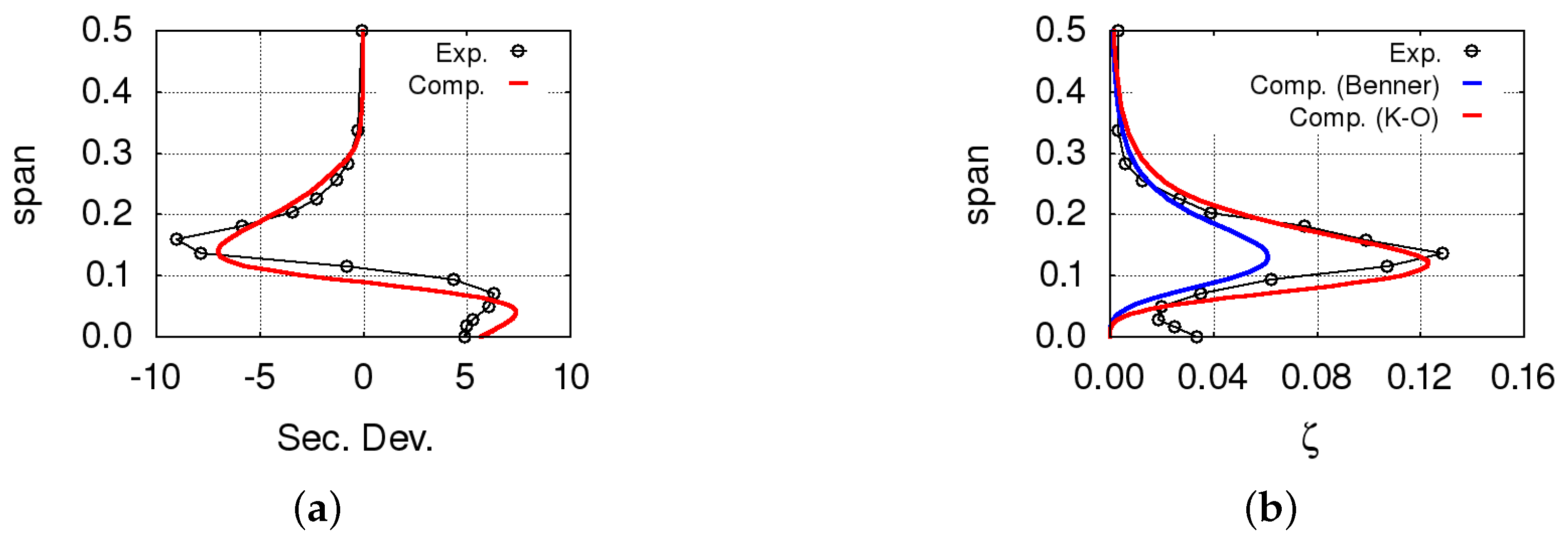
where , and h is measured as the spanwise distance from the endwalls. The vortex characteristic length (Figure 1b) is estimated at the blade trailing edge as a fraction of the secondary flow penetration depth in the spanwise direction Z: . The value of Z is estimated by using the Benner et al. correlation [13]. A value of has been chosen for the constant on the basis of numerical experiments and comparison with 3D CFD results (Figure 2). Inside the blade passage, the characteristic length is distributed linearly along the blade meridional length from the minimum blockage factor location up to the trailing edge. The circulation can then be expressed in terms of the vorticity at the vortex centre as: . The vorticity component is assumed to be coincident with the streamwise vorticity of the passage vortex. This is evaluated using the classical secondary flow theory (Hawthorne et al. [12]). However, it must be noted that in this theory such a vorticity contribution is considered as distributed in the blade passage and not concentrated at the vortex centre, as in the present approach. The secondary velocity component given by Equation (9) is finally projected in the tangential direction to obtain a tangential velocity which is then used in Equation (6) to generate an additional body force. This provides the secondary deviation distribution.
Secondary losses are estimated via correlations like the ones by Benner et al. [13] or Kacker and Okapuu [14]. Secondary loss coefficients are converted in entropy rise values , where local flow conditions at the endwalls are used for this purpose. Such values are then distributed in the spanwise direction so that the integral average of the distribution corresponds to , and the resulting entropy field is used for the distributed loss model. To this end, the following distribution function is used:
In practice, the function is normalized with its integral value between the endwall and midspan and multiplied by . It was found that Equation (10)—which is suggested by the behaviour of the dissipation in a Lamb–Oseen vortex—closely matches the results of viscous three-dimensional CFD calculations. In fact, several parametric studies were carried out in order to check the behaviour of the function and to determine the optimum value of the proportionality constant between the vortex characteristic length and the Benner et al. secondary flow penetration depth Z [13]. An example of these studies is summarized in Figure 2, where 3D CFD results are compared to throughflow predictions in terms of secondary deviation angle and loss coefficient. These quantities are defined as the difference between the actual flow quantities and the corresponding ones that would be obtained without secondary flow effects. Secondary losses are estimated with the Kacker–Okapuu correlation [14]. Results obtained with several values of the constant are reported.
5. Tip Leakage Model
In principle, tip clearance effects could be accounted for in the throughflow procedure in a fashion similar to that of secondary flows. Unfortunately, the correlations available for the tip vortex penetration depth in the spanwise direction and for the induced loss in flow turning by the blade row are characterized by a high level of empiricism and unsatisfactory agreement between different formulations (e.g., [15,16]). Therefore, it was decided to model tip leakage effects in terms of source and sink flux vectors and additional losses.
The sink and source terms are conceived in a form that conserves mass and energy while changing the momentum components in order to mimic tip leakage effects. They are introduced in the streamwise row of computational cells adjacent to the tip endwall in rotor blades. The height of those cells is enforced to be equal to the tip gap height by the grid generation procedure. For a computational cell in the tip gap, the total flux contribution in the direction of the computational plane becomes with:
where is defined in Equation (2) while are source/sink flux vectors. An analogous formulation holds for the flux contribution in direction.
The leakage mass flow rate is specified for the sink terms, while values of pressure and temperature are assumed equal to those of the main flow. For the source terms, the mass flow rate and the direction of the leakage flow are specified. This is assumed to be normal to the camber line of the tip section of the blade. Pressure is assumed to be equal to that of the main flow while the temperature is calculated so as to ensure energy conservation. The leakage mass flow rate through a tip clearance cell of area A is expressed by the formulation suggested by Denton [17] in the limit of incompressible leakage flow: . In this formula, is a discharge coefficient which is estimated with the correlation by Yaras and Sjolander [16], and is the pressure difference between the pressure and the suction side of the blade tip section. Such a quantity is related to the tangential component of the local blade body force, and it is estimated as: . The blade body force components are set to zero in the tip gap cells.
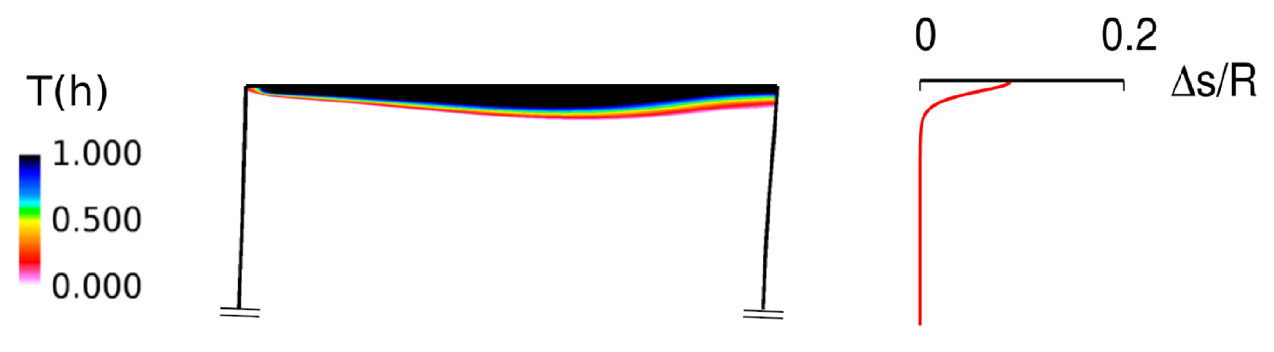
The tip leakage losses are computed from correlations and expressed in terms of entropy rise. These contributions are distributed linearly along the blade axial chord. In order to define a distribution in the spanwise direction, it is assumed that losses are concentrated where tip leakage effects are important. To identify these regions of the computational domain, a function of the spanwise coordinate is constructed as follows:
where and are given by Equations (5) and (9), respectively. Far from the tip gap-affected region, the tangential velocity component w is equal to due to the action of the body forces, and . Where the tangential momentum is modified by the effects of the source terms of Equation (11), w is different from and . As an example, contours of the T function and entropy distribution at the CT3 rotor trailing edge (see the following section) are reported in Figure 3.
6. Applications
6.1. T106 Cascade
The linear cascade under investigation is based on the T106 blade section, and was tested experimentally by Duden and Fottner [10] in a high speed wind tunnel in two configurations: one with parallel end walls and one with divergently tapered end walls. Due to the evidence of stronger secondary flow, the configuration discussed here is the tapered one. For the meridional analysis of linear cascades, the governing equations were recasted in a suitable form: the axisymmetric terms were dropped out, while blockage and body force source terms were reformulated and retained. The blade mean surface and the blockage distribution were obtained from the three-dimensional geometry of the cascade. The meridional channel was discretized with 120 grid cells in the axial direction, with 64 cells in the blade passage. Due to the symmetrical geometry of the endwalls and inlet conditions, only half of the blade height was considered, and it was discretized with 64 spanwise cells. Inlet boundary layer thicknesses and vorticity were deduced from the spanwise velocity distribution measured upstream of the cascade. They were used for the correlations by Benner et al., and Kacker–Okapuu for the secondary flow penetration depth and loss coefficient [13,14] and in the Hawthorne formula [12] for the streamwise vorticity at the trailing edge. The capability of the secondary flow model to produce realistic spanwise distributions can be appreciated in Figure 4, where computed secondary deviation and total pressure loss coefficient are compared to experiments. The experimental deviation distribution is quite well reproduced by the throughflow analysis. A secondary flow model with only one vortex cannot account for non symmetric effects, and for the analyzed configuration, this results in an underestimation of the flow underturning near the of the blade span. The prediction by the Benner et al. correlation for the spanwise penetration depth appears to be quite accurate. In terms of total pressure loss coefficient, the prediction based on the correlation by Kacker–Okapuu is in good agreement with measurements. Instead, the Benner et al. correlation results in a serious underestimation of the loss peak which is recorded near the of the span. The good reproduction of the shape of the loss distribution is remarkable, except for the first span where the experimental results are affected by the endwall boundary layer, which is not accounted for in the throughflow analysis.
6.2. CT3 Transonic Stage
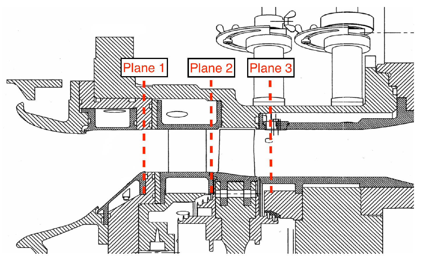
The CT3 high pressure stage was experimentally investigated at the von Kármán Institute (Rhode-Saint-Genèse, Belgium) in the framework of the TATEF2 EU funded project [18]. The turbine stage is composed of 43 cylindrical vanes and 64 unshrouded blades. A meridional view of the stage is reported in Figure 5.
Three operating conditions were tested during the measurement campaign. They are indicated as Nom (nominal), Low, and High conditions, and are characterized in Table 1 in terms of isentropic Mach numbers at stator and rotor exit, and stage total pressure ratio. Detailed experimental data were made available for Planes 1 and 3. The stage meridional channel was discretized with 256 grid cells in the axial direction and 64 in the spanwise direction. A number of 64 grid cells was used in the bladed regions of the computational domain. Profile deviations and losses were estimated via the Kacker–Okapuu correlation. Measured spanwise distributions at Plane 1 were used as boundary conditions and to determine the endwall boundary layers details for the secondary flow model. The Benner et al. correlation for the penetration depth and the Kacker–Okapuu formulation for secondary losses were used for the model closure. The mixing analysis proposed by Denton [17] was used to express tip leakage losses.
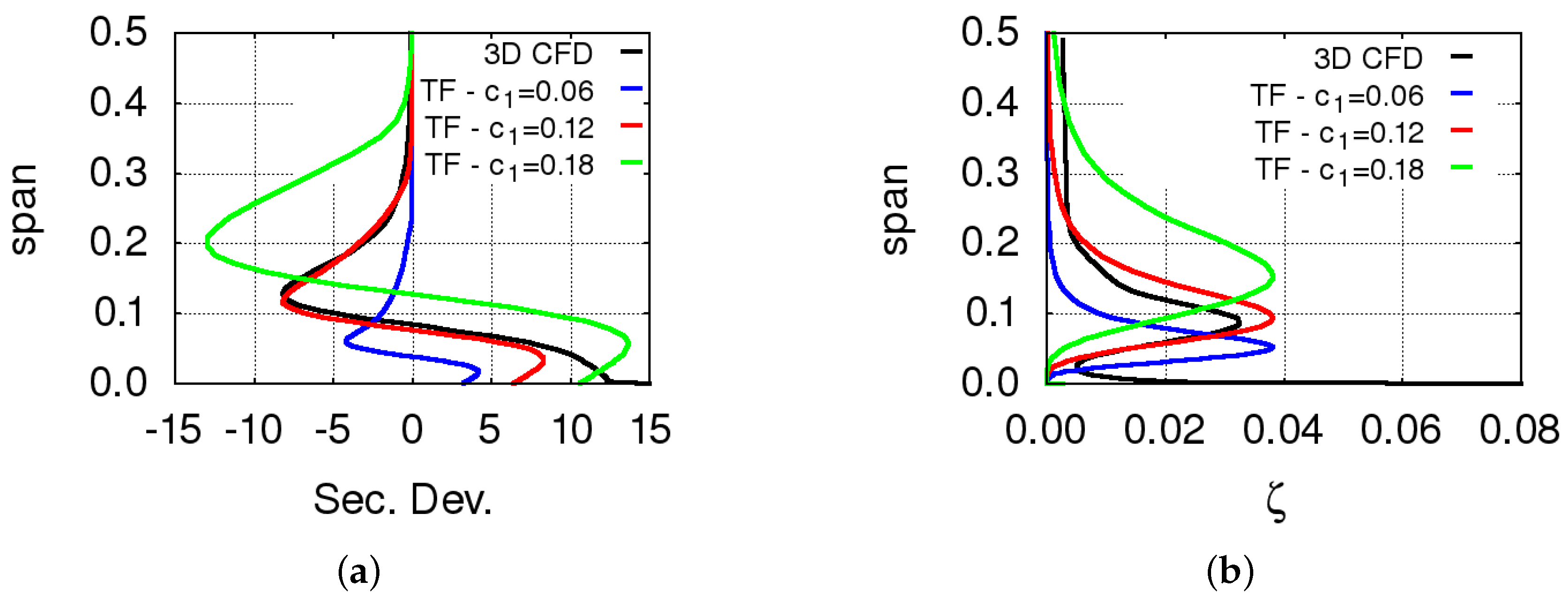
In terms of radial distributions of flow quantities, throughflow results obtained at the Nom condition with and without accounting for 3D effects are compared to experiments in Figure 6. The 3D steady viscous CFD results obtained with the TRAF code are also reported for comparison. The improvement in the predictions related to 3D flow features modeling is witnessed by a better agreement with experimental data. The comparison with 3D CFD results also reveals a good reproduction of the impact of three-dimensional effects on the meridional flow, even if spanwise distributions calculated with the TRAF code are significantly more distorted. The distortions associated with the strong secondary flow originating at the hub are not captured with the same accuracy for all the flow quantities. For example, in the first of the span, the agreement with measurements is quite good in terms of flow angle, but discrepancies appear in terms of absolute Mach number and total pressure. Similar conclusions can be drawn with reference to tip leakage effects. The predicted overshoots in flow quantities near the tip endwall are satisfactorily reproduced in magnitude, but the spanwise extent of such effects on Mach number and total pressure distributions looks underestimated with respect to the experimental data. The flow overturning shown by measurements between the and the of the span is not recorded by the throughflow analysis.
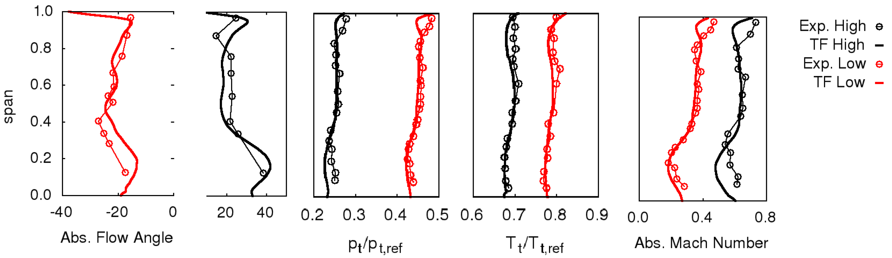
For the Low and High conditions, the level of agreement between throughflow predictions and experiments is practically the same. For those conditions, the comparison between calculated and measured radial distributions is shown in Figure 7. Relevant changes in the shape of the flow angle distribution and in the magnitude of the tip leakage-induced distortion occur when varying the stage expansion ratio. The realistic reproduction of such modifications—appreciable in Figure 6 and Figure 7—represents a remarkable merit of the proposed 3D flow features models.
In terms of stage output power (W) and total-to-total efficiency (), the comparison between computed and measured values is summarized in Table 2. Throughflow results with and without 3D models are reported. The computed mass flow rate value is equal to 9.31 kg/s for all three investigated operating conditions due to chocked flow in the vanes, and it is about higher than the experimental value of 9.15 kg/s.
The calculated power values are overestimated with respect to the experimental results. This is not surprising due to the comparable overestimation in mass flow rate. However, the discrepancy between predicted and measured values of the output power decreases from to about when 3D effects are accounted for in the throughflow analysis. The computed total-to-total efficiencies are also on a higher level with respect to measurements, but the trend with the stage expansion ratio is satisfactorily captured. This particular operating character of the CT3 stage has proven to be hardly predictable with accuracy, even by 3D unsteady viscous analyses [18]. Note that 12 seconds were needed to obtain a six decade drop of the root mean square (RMS) residuals in the throughflow analysis of the CT3 stage on a Intel® i7-4770 CPU @3.40 GHz (Dresden, Germany). A comparable convergence level in a steady, 3D, viscous, parallel calculation with the TRAF code requires a computational time of about half an hour on a reasonably coarse mesh.
7. Conclusions
The numerical results presented in the paper were aimed at assessing the feasibility of 3D flow features simulation in the context of a throughflow approach based on the axisymmetric Euler equations. Although the subject is not new, the proposed methodology attempts to address the issue with simple phenomenological models that naturally fit into the CFD-based structure of the throughflow solver. It is intended to provide a framework for the simulation of secondary flows and tip leakage effects, while leaving the task of estimating losses and other required bulk quantities to correlations. The treatment of secondary flows as transverse velocity fields generated by Lamb–Oseen-type vortices plus a realistic spanwise entropy distribution has proven to result in quite good secondary deviation and loss predictions on a linear cascade based on the T106 profile. A tip leakage model for unshrouded blades based on source/sink convective flux terms is also proposed. The two models—used in conjunction with fairly standard correlations for profile losses and deviations—led to improved predictions of the circumferentially averaged flow structure of the CT3 transonic stage. Calculated radial distributions of flow properties and stage performance were found to be at least in qualitative agreement with experiments not only at design conditions, but also when studying off-design trends. Non-negligible discrepancies are also found near the endwalls in the radial distributions of some parameters. This would suggest that the discussed models are too crude to correctly reproduce the complex mechanisms of spanwise redistribution occurring in highly loaded low aspect ratio turbine stages. Nonetheless, it is believed that the performance of the proposed methodology is in line with the requirements of fast engineering predictions for the design of axial turbines.
Acknowledgments
We would like to thank our fellow partners in European Union FP6 programme TATEF2 (Contract No. AST3-CT-2004-502924) for permitting the publication of our results in this paper.
Author Contributions
Roberto Pacciani and Michele Marconcini contributed equally to the work described in the manuscript. Andrea Arnone supervised the work and provided editorial inputs for the manuscript.
Conflicts of Interest
The authors declare no conflict of interest.
Nomenclature
Latin Symbols
| A | tip gap area |
| b | tangential blockage factor |
| tip leakage discharge coefficient | |
| d | dissipating body force |
| inviscid flux vectors | |
| f | blade body force |
| H | specific total enthalpy |
| J | Jacobian |
| M | Mach number |
| m | meridional coordinate |
| mass flow rate | |
| N | number of blades |
| p | pressure |
| R | gas constant |
| r | radius |
| source term vector | |
| s | specific entropy |
| intrinsic coordinates | |
| T | absolute temperature, leakage loss distribution function |
| t | time |
| u | axial velocity |
| contravariant velocities in and directions | |
| v | radial velocity |
| W | power |
| w | tangential velocity |
| cylindrical coordinates | |
| Z | secondary flow penetration depth |
| vortex characteristic length |
Greek Symbols
| vortex circulation, streamsurface | |
| efficiency | |
| normalized spanwise coordinate, loss coefficient, | |
| kinematic fluid viscosity | |
| curvilinear coordinates | |
| fluid density | |
| secondary loss distribution function | |
| angular velocity | |
| vorticity |
Subscripts
| 1, 2 | cascade inlet, outlet |
| b | blockage-related |
| f | force-related |
| isentropic | |
| pressure side | |
| reference | |
| pressure side | |
| t | total quantity |
Superscripts
| T | transposed |
Abbreviations
| CFD | Computational Fluid Dynamics |
| EU | European Union |
| RMS | Root Mean Square |
| TATEF2 | Turbine Aero-Thermal External Flows |
| TF | Throughflow |
References
- Smith, L.H. The Radial-Equilibrium Equation of Turbomachinery. J. Eng. Gas Turb. Power 1966, 88, 1–12. [Google Scholar] [CrossRef]
- Novak, R.A. Streamline Curvature Computing Procedures for Fluid Flow Problems. J. Eng. Gas Turb. Power 1967, 89, 478–490. [Google Scholar] [CrossRef]
- Sturmayr, A.; Hirsch, C. Shock Representation by Euler Throughflow Models and Comparison with Pitch-Averaged Navier-Stokes Solutions. In Proceedings of the Fourteenth International Symposium on Breathing Engines (ISABE), Florence, Italy, 5–10 September 1999; American Institute of Aeronautics and Astronautics: Reston, VA, USA, 1999; pp. 99–7281. [Google Scholar]
- Simon, J.F.; Léonard, O. A Throughflow Analysis Tool Based on the Navier-Stokes Equations. In Proceedings of the 6th European Turbomachinery Conference, Lille, France, 7–11 March 2005. [Google Scholar]
- Pacciani, R.; Rubechini, F.; Marconcini, M.; Arnone, A.; Cecchi, S.; Daccà, F. A CFD-Based throughflow Method with an Explicit Body Force Model and an Adaptive Formulation for the S2 Streamsurface. P. I. Mech. Eng. A-J. Pow. 2016, 230, 1–13. [Google Scholar] [CrossRef]
- Pasquale, D.; Persico, G.; Rebay, S. Optimization of Turbomachinery Flow Surfaces Applying a CFD-Based Throughflow Method. J. Turbomach. 2012, 136, 031013. [Google Scholar] [CrossRef]
- Petrovic, M.V.; Widermann, A. Through-Flow Analysis of Air-Cooled Gas Turbines. In Proceedings of the ASME Turbo Expo, Copenhagen, Denmark, 11–15 June 2012. ASME Paper No. GT2012-69854. [Google Scholar]
- Arnone, A. Viscous Analysis of Three-Dimensional Rotor Flow Using a Multigrid Method. J. Turbomach. 1994, 116, 435–445. [Google Scholar] [CrossRef]
- Wu, C.H. A General Theory of Three-Dimensional Flow in Subsonic and Supersonic Turbomachines of Axial-, Radial-, and Mixed-Flow Types; NACA TN 2604; National Advisory Commitee for Aeronautics: Cleveland, OH, USA, 1952. [Google Scholar]
- Duden, A.; Fottner, L. Influence of Taper, Reynolds Number and Mach Number on the Secondary Flow Field of a Highly Loaded Turbine Cascade. P. I. Mech. Eng. A-J. Pow. 1997, 211, 309–320. [Google Scholar] [CrossRef]
- Jameson, A.; Schmidt, W.; Turkel, E. Numerical Solutions of the Euler Equations by Finite Volume Methods Using Runge–Kutta Time–Stepping Schemes. In Proceedings of the AIAA 14th Fluid and Plasma Dynamics Conference, Palo Alto, CA, USA, 23–25 June 1981. AIAA Paper 81-1259. [Google Scholar]
- Hawthorne, W.R.; Armstrong, W.D. Rotational Flow through Cascades, Part II: The Circulation about the Cascade. Q. J. Mech. Appl. Math. 1955, 8, 280–292. [Google Scholar] [CrossRef]
- Benner, M.W.; Sjolander, S.A.; Moustapha, S.H. An Empirical Prediction Method for Secondary Losses in Turbines—Part I: A New Loss Breakdown Scheme and Penetration Depth Correlation. J. Turbomach. 2006, 128, 273–280. [Google Scholar] [CrossRef]
- Kacker, S.C.; Okapuu, U. A Mean Line Prediction Method for Axial Flow Turbine Efficiency. ASME J. Eng. Power 1982, 104, 111–119. [Google Scholar] [CrossRef]
- Rains, D.A. Tip Clearance Flows in Axial Flow Compressors and Pumps. Ph.D. Thesis, California Institute of Technology, Pasadena, CA, USA, 1954. [Google Scholar]
- Yaras, M.I.; Sjolander, S.A. Prediction of Tip—Leakage Losses in Axial Turbines. J. Turbomach. 1992, 114, 204–210. [Google Scholar] [CrossRef]
- Denton, J.D. The 1993 IGTI Scholar Lecture—Loss Mechanisms in Turbomachines. J. Turbomach. 1993, 115, 621–656. [Google Scholar] [CrossRef]
- Paniagua, G.; Yasa, T.; de la Loma, A.; Coton, T. Unsteady Strong Shock Interactions in a Transonic Turbine: Experimental and Numerical Analysis. J. Propul. Power 2008, 24, 722–731. [Google Scholar] [CrossRef]
Figure 1.
(a) Sketch of a blade row with the intrinsic coordinate system; and (b) Lamb–Oseen vortex and secondary velocities.
Figure 1.
(a) Sketch of a blade row with the intrinsic coordinate system; and (b) Lamb–Oseen vortex and secondary velocities.
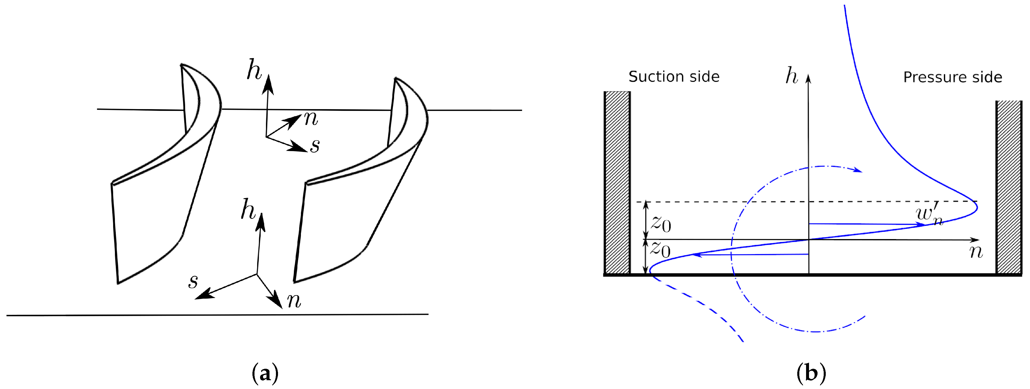
Figure 2.
Comparisons between 3D computational fluid dynamics (CFD) and throughflow results in terms of spanwise distributions of (a) secondary deviation angle [deg] and (b) loss coefficient for different values of the constant.
Figure 2.
Comparisons between 3D computational fluid dynamics (CFD) and throughflow results in terms of spanwise distributions of (a) secondary deviation angle [deg] and (b) loss coefficient for different values of the constant.

Figure 3.
Tip clearance loss distribution and entropy at the trailing edge of the CT3 rotor.

Figure 4.
Predicted and measured spanwise distributions of (a) secondary deviation angle [deg] and (b) loss coefficient for the T106 cascade with tapered endwalls [10].
Figure 4.
Predicted and measured spanwise distributions of (a) secondary deviation angle [deg] and (b) loss coefficient for the T106 cascade with tapered endwalls [10].

Figure 5.
Meridional view of the CT3 stage.

Figure 6.
Predicted and measured spanwise distributions of flow quantities in Plane 3 for the CT3 stage at Nom condition with and without 3D effects (abs. flow angle expressed in [deg]).
Figure 6.
Predicted and measured spanwise distributions of flow quantities in Plane 3 for the CT3 stage at Nom condition with and without 3D effects (abs. flow angle expressed in [deg]).
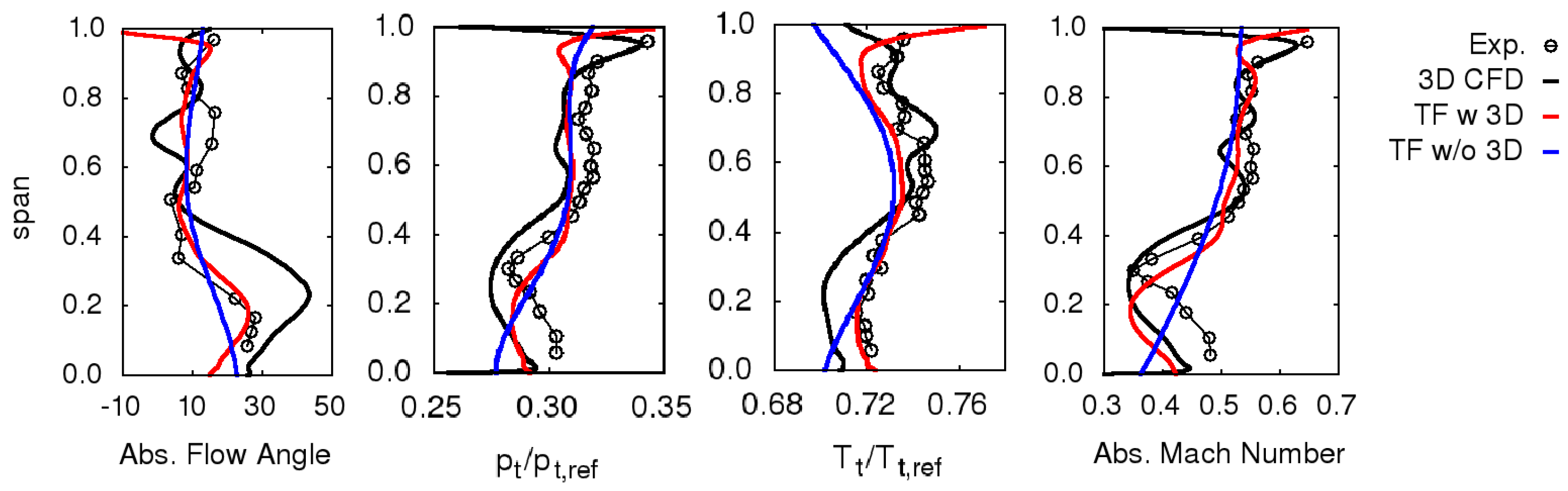
Figure 7.
Predicted and measured spanwise distributions of flow quantities in Plane 3 for the CT3 stage at High and Low conditions (abs. flow angle expressed in [deg]).
Figure 7.
Predicted and measured spanwise distributions of flow quantities in Plane 3 for the CT3 stage at High and Low conditions (abs. flow angle expressed in [deg]).


Table 1.
Operating conditions for the CT3 stage.
| Low | |||
| Nom | |||
| High |
Low: low pressure ratio, Nom: nominal pressure ratio, High: high pressure ratio.
Table 2.
Measured and computed performance for the CT3 stage.
| W (kW) | ||
|---|---|---|
| Low: Exp./ TF w 3D/ TF w/o 3D | ||
| Nom: Exp./ TF w 3D/ TF w/o 3D | ||
| High: Exp./ TF w 3D/ TF w/o 3D |
Low: low pressure ratio, Nom: nominal pressure ratio, High: high pressure ratio, Exp: experimental value, 3D: three-dimensional flow features.
© 2017 by the authors. Licensee MDPI, Basel, Switzerland. This article is an open access article distributed under the terms and conditions of the Creative Commons Attribution (CC BY-NC-ND) license (https://creativecommons.org/licenses/by-nc-nd/4.0/).
Share and Cite
MDPI and ACS Style
Pacciani, R.; Marconcini, M.; Arnone, A. A CFD-Based Throughflow Method with Three-Dimensional Flow Features Modelling. Int. J. Turbomach. Propuls. Power 2017, 2, 11. https://doi.org/10.3390/ijtpp2030011
AMA Style
Pacciani R, Marconcini M, Arnone A. A CFD-Based Throughflow Method with Three-Dimensional Flow Features Modelling. International Journal of Turbomachinery, Propulsion and Power. 2017; 2(3):11. https://doi.org/10.3390/ijtpp2030011
Chicago/Turabian StylePacciani, Roberto, Michele Marconcini, and Andrea Arnone. 2017. "A CFD-Based Throughflow Method with Three-Dimensional Flow Features Modelling" International Journal of Turbomachinery, Propulsion and Power 2, no. 3: 11. https://doi.org/10.3390/ijtpp2030011