Development and Implementation of a Technique for Fast Five-Hole Probe Measurements Downstream of a Linear Cascade ^†

Abstract

Flow measurement using a linear compressor or turbine cascade is a well-established technique to characterize the flow in turbomachines with a certain degree of abstraction. A common way to obtain a general characterization of the flow is to measure the flow downstream of the cascade with a five-hole probe, obtaining, e.g., total pressure losses and flow turning. Pneumatic five-hole probes are used to capture steady or time-averaged flow quantities, if not specified otherwise. In dependency of probe geometry, measurement set-up and flow properties, such measurements can be very time-consuming. Various techniques, in order to decrease the measurement time, are proposed in literature but for certain applications the efforts required to implement such techniques can outweigh the enhanced measurement speed. In this paper, methods proposed by other authors are combined and extended to allow for fast or transient five-hole probe measurements at strongly varying flow conditions. The effectiveness of this method is presented for flow measurements downstream of a compressor cascade with attached and stalled flow (by varying the Reynolds number) as well as with steady and periodically unsteady inflow. The new method allows to reduce the measurement time by up to 90 percent without compromising measurement accuracy. In fact, due to higher spatial resolution, the flow downstream of the cascade can be better resolved with the new method.

1. Introduction

Pneumatic probes have been widely used in fluid mechanics research and are still a valuable measurement device for obtaining localized flow quantities such as total pressure, Mach number or flow angle. In turbomachinery research, pneumatic probes with two, three, five or even more holes are used to measure the flow properties in annular as well as linear cascades or even rotating rigs. The pressure at each of the holes is measured and the relation between the individual pressures allows to obtain the flow properties according to the values from a prior calibration.

For a standard pneumatic multi-hole probe, the pressure is not measured directly at the holes. The hole is connected via small diameter tubes and hoses to the actual pressure transducer. At steady conditions, the pressure inside the cavity of the pressure transducer is the same as at the hole. For a pressure change at the hole, it takes a certain time to equalize the pressure difference between hole and pressure sensor. For accurate measurements, one has to take this time lag into account when traversing a probe in a non-homogeneous flow. Depending on the kind of flow and the measurement set-up, this time lag can be responsible for most of the time needed to measure a flow field. In order to reduce measurement time and hence the costs, it is important to find solutions which allow to minimize the settling time of the pressure changes. One way to shorten the measurement time is to use highly time-resolving pneumatic probes, where the pressure sensors are placed more or less directly at the probe tip. As drawbacks, these probes are usually more expensive than standard probes, are more difficult to handle and have larger dimensions. The latter is due to the need to incorporate the sensors inside the probe, either at the tip or shortly downstream. Additionally, the operating range of the probe may be limited to the sensors’ operating range if the design does not allow to change them easily.

If one wants to use a standard probe, one can optimize the measurement set-up, as carried out, e.g., in Grimshaw and Taylor [1]. The authors use an electric circuit analogy to model the complete pressure lines and are able to estimate the pressure settling time and to derive optimized geometries or configurations. Nevertheless, such an optimization will face restrictions such as the size of the probe already in use and the minimum tube length from the probe to the sensor. Another or an additional way to reduce measurement time is to by-pass the pressure settling time by applying a transfer function to the pressure record as in Paniagua and Dénos [2]. For their method, they traverse the probe continuously through the flow field and measure the pressure throughout the traverse. The pressure at the sensor is not allowed to settle down and is therefore not equal to the pressure at the probe tip. Since they made a prior calibration acquiring the response of the measurement set-up to a step change in pressure at the probe tip, they are able to reconstruct the actual pressure at the tip applying a transfer function on the pressure history of the sensor. This method allows to reduce the measurement time considerably, but requires a calibration of the system to obtain the transfer function. Such a calibration has to be done not only for different measurement set-ups individually but also for different flow conditions. The absolute pressure level at which the system is working has a huge influence on the response of the system; therefore, measurements at different pressure levels require individual calibrations. Such additional efforts may outweigh the advantages of a continuous measurement and hence are not suitable for measurements under strongly varying pressure levels.

At the High-Speed Cascade Wind Tunnel of the Institute of Jet Propulsion of the Armed Forces University Munich, flow measurements with pneumatic probes using linear turbine and compressor cascades are often carried out for different operating points with a large variation of pressure level. A dynamic calibration for every measurement would represent an effort as high or even higher than a standard measurement of a traverse at mid-span waiting for the pressure settling time for each measurement point. In order to improve the overall time needed for the measurement, a transfer function based on the method of Paniagua and Dénos [2] is applied to the measurement using the values of the measurement itself to obtain the transfer function.

2. Settling Time and Transfer Function Method

The determination of the settling time for pressure measurement systems has been the focus of study since quite early on in the history of wind tunnel testing. The settling time is important whenever there is a noticeable time lag between pressure changes at the measurement location and the actual measurement device. Sinclair and Robins [3] developed an equation for the determination of settling time for laminar, incompressible flow measured by a manometer. The measured pressure at the measurement device—in the case of this reference, a manometer, but it can also be a pressure gauge—is a function of time $p=f\left(t\right)$. At $t=0$, the system is in equilibrium at $p=p_0$. After a step change at the orifice of the measurement system (e.g., a probe tip) from $p_0$ to $p_1$, the measured value will change. The settling time can be defined as time needed for the measured pressure to level 99.9% of the initial pressure difference $p_1-p_0$, i.e.,

$$p_s=0.999·p_1+0.001·p_0.$$

(1)

In [3], the settling time $t_p$ is given as

$$t_p=\frac{128\mu l_e}{\pi d^4}\left[\frac{V}{p_1}ln\frac{\left(p_0-p_1\right)\left(p_s+p_1\right)}{\left(p_s-p_1\right)\left(p_0+p_1\right)}+\frac{3V_d}{p_0-p_1}ln\frac{p_0+p_1}{p_s+p_1}+\frac{V_d}{p_0-p_1}ln\frac{p_0-p_1}{p_s-p_1}\right],$$

(2)

with the natural logarithm ln, the total volume of the system V and the displacement volume due to fluid level change in the manometer $V_d$. The equivalent length $l_e$ is determined for a combination of different tube diameters $d_i$ by

$$l_e=l_1+l_2\frac{d^4}{d_2^4}+l_3\frac{d^4}{d_3^4}+\dots +l_n\frac{d^4}{d_n^4}.$$

(3)

Larcombe and Peto [4] derive the settling time for slip flow as

$$t_p=\frac{128\mu \left(V+kv\right)l}{\pi d^4\left(p_1+K\right)}\left[ln\frac{p_1+p_s}{p_1-p_s}-ln\frac{p_1+p_0}{p_1-p_0}+ln\frac{1+\frac{2K}{p_1+p_s}}{1+\frac{2K}{p_1+p_0}}\right],$$

(4)

with

$$K=8{\left(\frac{\pi }{2}\right)}^{0.5}\left(\frac{2}{f}-1\right)\frac{\mu }{d{\left(\frac{\rho }{p}\right)}^{0.5}}$$

(5)

where $kv$ is equivalent to $V_d$ in Equation (2) and f is the fraction of gas molecules diffusely reflected. In the reference, f is suggested to be equal to 0.8 for air at 20 ${}^{\circ }$C. The equivalent length for a combination of various diameters is given as

$$l_e=l+\underset{i=1}{\sum ^n}\frac{l_i{d}^4\left(p_1+K\right)}{d_i^4\left(p_1+K_i\right)}\frac{ln\frac{199p_1+p_0+200K_i}{p_1+p_0+2K_i}}{ln\frac{199p_1+p_0+200K}{p_1+p_0+2K}}.$$

(6)

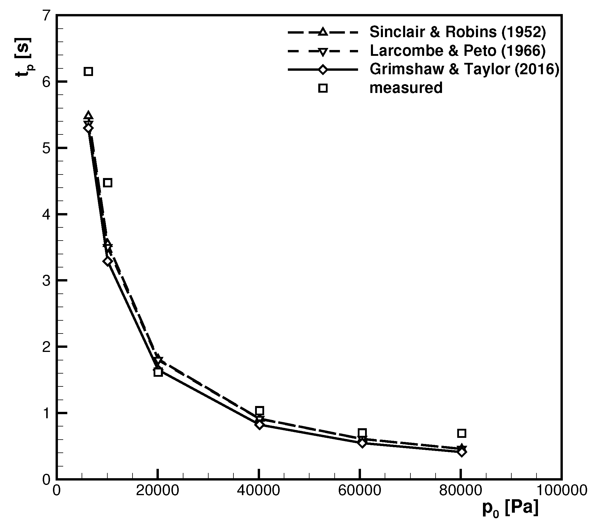
In a recent publication, Grimshaw and Taylor [1] use an electric circuit analogy to derive the set of differential equations for the determination of the pressure history. Though the results in their absolute values might differ from each other, altogether they show a strong dependency of the settling time from the absolute pressure level. Figure 1 shows the settling time dependency on the overall pressure level $p_0$ for a typical measurement configuration in a wind tunnel, applying the theories discussed so far. The strong increase of the settling time with decreasing pressure level seems evident. The configuration of the measurement set-up for a single pressure hole of the five-hole probe is explained in

Table 1. Typical probe and connecting tube dimensions for the five-hole probe set-up.

	l	d
probe tip	5 mm	0.4 mm
probe stem	230 mm	0.55 mm
connecting tube	1000 mm	1.5 mm
transducer tube	100 mm	1 mm

, while the applied pressures are given in

Table 2. Pressure boundary conditions for evaluation of the settling time.

${\mathit{p}}_0$	${\mathit{p}}_1-{\mathit{p}}_0$
80,200 Pa	1100 Pa
60,500 Pa	750 Pa
40,170 Pa	670 Pa
20,080 Pa	540 Pa
10,080 Pa	460 Pa
6260 Pa	590 Pa

. Overall, the probe head has a diameter of 2.5 mm.

Some validation measurements were carried out with a simple set-up and a manual valve to produce a sudden pressure increase from $p_0$ to $p_1$ at the five-hole probe tip. A Kulite (Leonia, NJ, USA) pressure sensor placed close to the probe tip is used as a reference signal to capture the actual pressure increase. The fast reacting pressure sensor is of the type XCQ-062 and has a natural frequency of 150 kHz with a differential pressure range of 350 hPa. Overall, the measurements confirm the trend predicted by the cited authors as shown in Figure 1. Viscous effects might be responsible for the slight increase in settling time in the experiments.

One may try to reduce the settling time as carried out, e.g., in [3] or [1] by optimizing the tube diameters, but physical limitations and constraints to the set-up will always lead to considerable time consumption of measurements with standard pneumatic probes, especially at low pressure levels.

2.1. Continuous Traverse Using Transfer Function

Paniagua and Dénos [2] present a method using a transfer function to obtain the true pressure at the probe tip. Simplifying and neglecting any time delay between step change and pressure rise at the transducer, one can reconstruct the true pressure from the time history of the true pressure and the measured pressure. For a measurement at a sampling time instance j, the true pressure u is obtained by

$$u_j=-b_1·u_{j-1}-\dots -b_m·u_{j-m}+a_0·y_j+a_1·y_{j-1}+\dots +a_m·y_{j-m}$$

(7)

with the order of the function m and the measured pressure y. A probe might then be traversed continuously through an inhomogeneous flow field and the actual pressure at each of the holes reconstructed by the measured pressure. For such an operation, one must know the coefficients $b_1\dots b_m$ and $a_0\dots a_m$, which can be obtained by prior calibration, as shown by the same authors. However, if one is carrying out measurements at different pressure levels, this would imply a calibration for each pressure level, which would outweigh any time savings by this method.

A more suitable way for measurements under varying pressure conditions is to obtain the coefficients from the measurement itself, bypassing any calibration. Therefore, a method proposed by Bartsch et al. [5] for optimization of the measurement point distribution for standard measurements is used here to determine the coefficients of the transfer function. In the publication from Bartsch et al. [5], they perform two traverses in opposite directions downstream of an airfoil in order to determine the wake position and to enhance the measurement point distribution for a standard traverse.

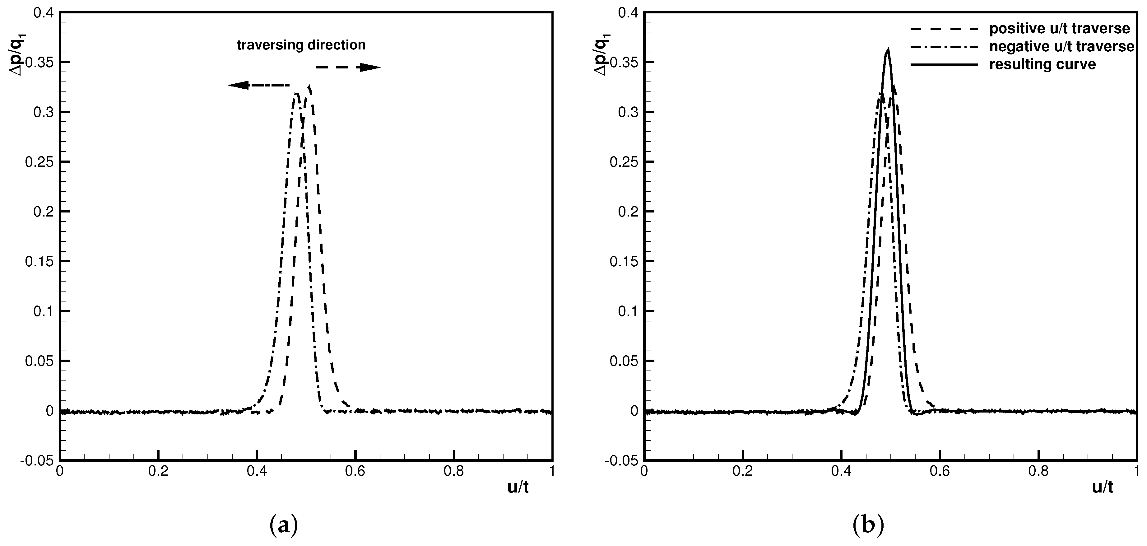
Such a dual traverse can also be used to directly obtain the actual pressure at each measurement location. In Figure 2a, typical results for a dual traverse are plotted. The dashed line shows the measured pressure difference between total inlet pressure and the pressure at the centre hole of the probe normalized by a random stagnation pressure for a continuous traverse toward higher $u/t$ values. The dashed–dotted line shows similar readings for a traverse in the same flowfield but moving in the opposite direction. It is evident that the time delay between actual pressure change and measured pressure leads to a phase lag of the measured pressure, seen in the different positions of the peak values. Additionally, the measured pressure difference is expected to be lower than the actual maximum. The coefficients for the transfer function in Equation (7) can be evaluated iteratively and the function applied to both traverses must give the same result, or more precisely

$${\mathbf{u}}_f-{\mathbf{u}}_s={\mathsf{\Psi }}_f·\mathsf{\phi }-{\mathsf{\Psi }}_s·\mathsf{\phi }=\mathsf{\xi }$$

(8)

with the vectors of the measured pressures $\mathbf{u}={\left[u_m,\cdots ,u_n\right]}^T$ for n measurement points and with the subscripts f and s for the first respectively second traverse. The vector $\mathsf{\phi }={\left[-b_1,\cdots ,-b_m,a_0,\cdots ,a_m\right]}^T$ holds the coefficients of the transfer function while the matrix $\mathsf{\Psi }$ is defined as

$$\mathsf{\Psi }=\left[\begin{array}{cccccc}{u}_{m-1}& \cdots & u_1& y_m& \cdots & y_1\\ ⋮& & & & & ⋮\\ u_{n-1}& \cdots & u_{n-m}& y_n& \cdots & y_{n-m}\end{array}\right].$$

(9)

The coefficients of the vector $\mathsf{\phi }$ in Equation (8) are iteratively searched to minimize the root mean square of the error vector $\mathsf{\xi }$ using the MatLab (MathWorks, Natick, MA, USA) function fminsearch. The order of the function m can be individually set for each experiment, but in our measurements an order higher than $m=3$ did not change the results significantly.

Since the number of coefficients for $\mathsf{\phi }$ is in general higher than two, additional constraints are put into the algorithm for the iterative search: the resulting actual pressure history as a function of $u/t$ has to cross all measured pressure difference peaks, i.e., maximum and minimum values, if this is the case. This is true, since the traversing velocity is moderate which results in macroscopic pressure changes, like the peaks in Figure 2a, far below one Hertz. According to the works of Bergh and Tijdeman [6] or Carolus [7] at such low frequencies and since the system is overdamped, no noticeable phase lag is perceived for the pressure reverse at the tip of the probe. The resulting pressure line for the curves shown in Figure 2a is plotted in Figure 2b together with the measured curves.

Such an iterative search can be done for all the holes or measured pressure differences of the five-hole probe and the actual flow values can be computed. Additional smoothing of the obtained values by a moving average filter of window size equal to the order of the transfer function allows to decrease the wiggles due to overestimation of random variations in the pressure measurement.

2.1.1. Error Estimation

An error estimation is more difficult to conduct using the transfer function since every computed pressure difference relies on the history of the measured and reconstructed pressure values $u_j=f(u_{j-1},\dots ,u_{j-m},y_j,\dots ,y_{j-m})$. This means that every error in previous samples propagates to the following pressures. Using the linear error propagation technique, which is the more conservative approach, without any further analysis would very soon increase the uncertainty towards infinity, since

$$\mathrm{\Delta }{u}_j=|-b_1|·\mathrm{\Delta }{u}_{j-1}+\dots +|-b_m|·\mathrm{\Delta }{u}_{j-m}+|a_0|·\mathrm{\Delta }{y}_j+\dots +\left|a_m\right|·\mathrm{\Delta }{y}_{j-m},$$

(10)

with $\mathrm{\Delta }y$ as the uncertainty of the pressure gauge, i.e., $\mathrm{\Delta }{y}_j=\mathrm{\Delta }{y}_{j-1}=\dots =\mathrm{\Delta }y$. However, one can overcome this problem if one separates the systematic from the random error with

$$\mathrm{\Delta }{y}_j=\overline{\mathrm{\Delta }y}+\mathrm{\Delta }{y}_j^{\prime },\mathrm{with}\underset{j=1}{\sum ^{\infty }}\mathrm{\Delta }{y}_j^{\prime }=0.$$

(11)

The systematic error is constant for all samples; therefore, Equation (10) can be rewritten as

$$\begin{array}{cc}\hfill \mathrm{\Delta }{u}_j=& |-b_1|·\mathrm{\Delta }{u}_{j-1}+\dots +|-b_m|·\mathrm{\Delta }{u}_{j-m}+\hfill \\ & |a_0+\dots +a_m|·\overline{\mathrm{\Delta }y}+|a_0|·\mathrm{\Delta }{y}_j^{\prime }+\dots +\left|a_m\right|·\mathrm{\Delta }{y}_{j-m}^{\prime }.\hfill \end{array}$$

(12)

The effect of such a method can be seen exemplary for a case of the order $m=1$ for simplification. The first transformation is at the second sample

$$\begin{array}{ccc}\hfill u_2& =& -b_1·u_1+a_0·y_2+a_1·y_1\hfill \end{array}$$

(13)

$$\begin{array}{cc}\hfill \mathrm{\Delta }{u}_2& =|a_1-b_1|·\mathrm{\Delta }{y}_1+\left|a_0\right|·\mathrm{\Delta }{y}_2\hfill \\ & =|a_0+a_1-b_1|·\overline{\mathrm{\Delta }y}+|a_1-b_1|·\mathrm{\Delta }{y}_1^{\prime }+\left|a_0\right|·\mathrm{\Delta }{y}_2^{\prime },\hfill \end{array}$$

(14)

since at the first sample the probe is not in motion and the measured pressure can be seen as the actual pressure at the probe tip $u_1=y_1$. For the third reading, the result from Equation (15) is set into the error estimation of Equation (12)

$$\begin{array}{ccc}\hfill \mathrm{\Delta }{u}_3& =& |-b_1|·\mathrm{\Delta }{u}_2+|a_0|\mathrm{\Delta }{y}_3+\left|a_1\right|·\mathrm{\Delta }{y}_2\hfill \\ & =& |(a_0+a_1)·(1+b_1)-b_1^2|·\overline{\mathrm{\Delta }y}+\hfill \\ & & |b_1(a_1-b_1)|·\mathrm{\Delta }{y}_1^{\prime }+\left(\right|b_1{a}_0|+|a_1\left|\right)·\mathrm{\Delta }{y}_2^{\prime }+\left|a_0\right|·\mathrm{\Delta }{y}_3^{\prime }.\hfill \end{array}$$

(15)

Applying the same method into the fourth reading gives

$$\begin{array}{cc}\hfill \mathrm{\Delta }{u}_4=& |(a_0+a_1)·(1+b_1+b_1^2)-b_1^3|·\overline{\mathrm{\Delta }y}+\hfill \\ & +|b_1^2(a_1-b_1)|·\mathrm{\Delta }{y}_1^{\prime }+\left(\right|b_1^2{a}_0|+|b_1{a}_1\left|\right)·\mathrm{\Delta }{y}_2^{\prime }+\hfill \\ & +\left(\right|b_1{a}_0|+|a_1\left|\right)·\mathrm{\Delta }{y}_3^{\prime }+\left|a_0\right|·\mathrm{\Delta }{y}_4^{\prime }.\hfill \end{array}$$

(16)

Continuing the row, one can easily find the relation

$$\begin{array}{cc}\hfill \mathrm{\Delta }{u}_j=& \overline{\mathrm{\Delta }y}\left|\underset{n=0}{\sum ^{j-2}}\left(a_0+a_1\right)b_1^n-b_1^{j-1}\right|+\hfill \\ & \underset{n=2}{\sum ^{j-1}}\mathrm{\Delta }{y}_n^{\prime }\left(|a_0·b_1^{j-n}|+|a_1·b_1^{j-n-1}|\right)+\mathrm{\Delta }{y}_0^{\prime }|a_1·b_1^{j-2}-b_1^{j-1}|.\hfill \end{array}$$

(17)

The first summand of Equation (17) can be brought to a geometric series for $b_1\ne 1$ with

$$\overline{\mathrm{\Delta }y}\left|\underset{n=0}{\sum ^{j-2}}\left(a_0+a_1\right)b_1^n-b_1^{j-1}\right|=\overline{\mathrm{\Delta }y}\left|(a_0+a_1)\frac{b_1^{j-1}-1}{b_1-1}-b_1^{j-1}\right|.$$

(18)

Equation (18) does not converge for $|b_1|>1$. It is therefore mandatory to find coefficients $b_n$ where the sum of the absolute values is smaller than unity in order to maintain mathematically correctly the uncertainty at low levels. Otherwise, the uncertainty grows exponentially with the number of data points.

The fluctuating random error (second and third summand in Equation (17)) is essentially due to noise and can, in general, be neglected for the average values, since the sum of the errors is equal to zero, see Equation (11).

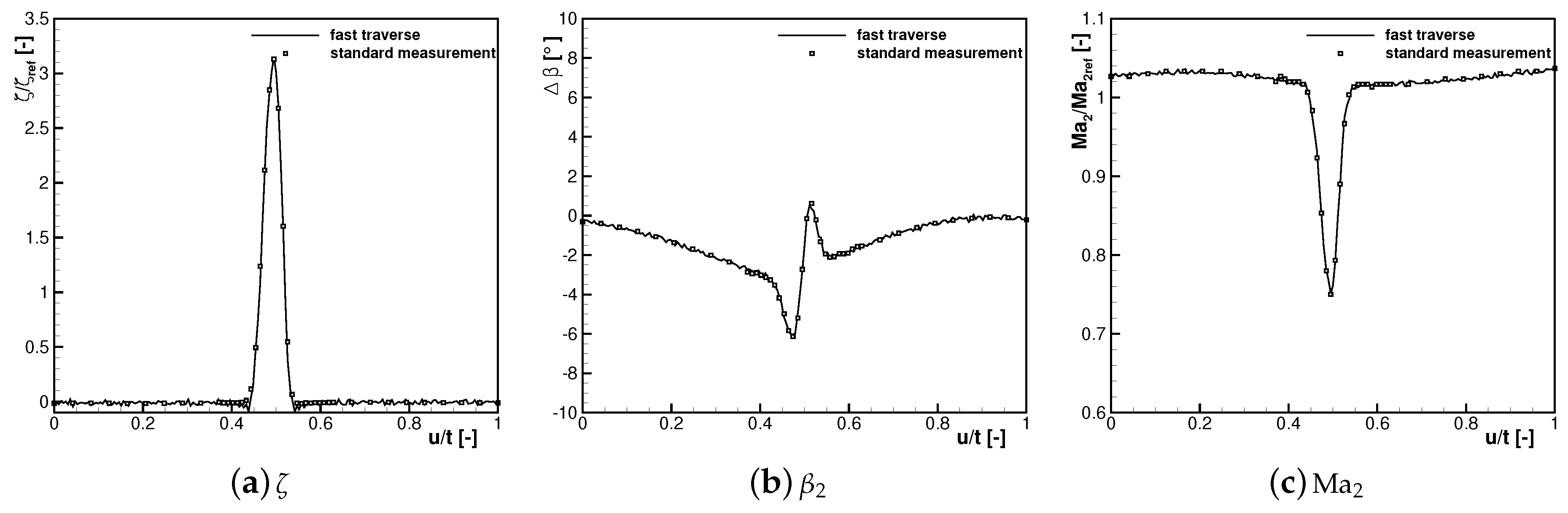
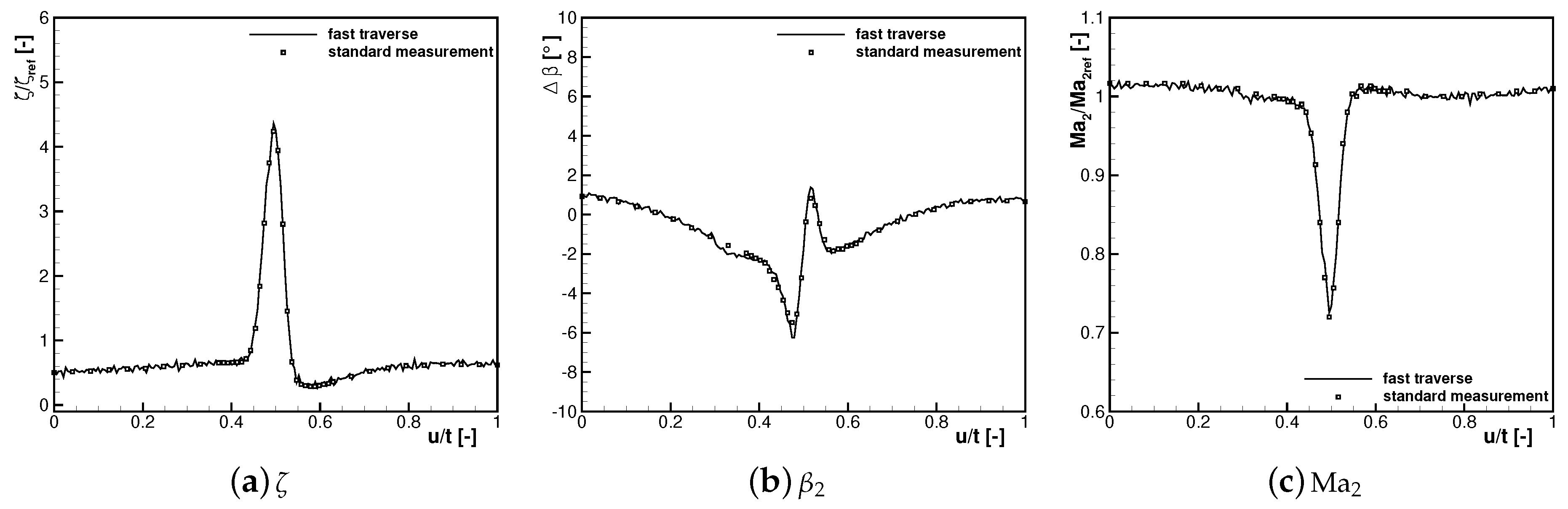
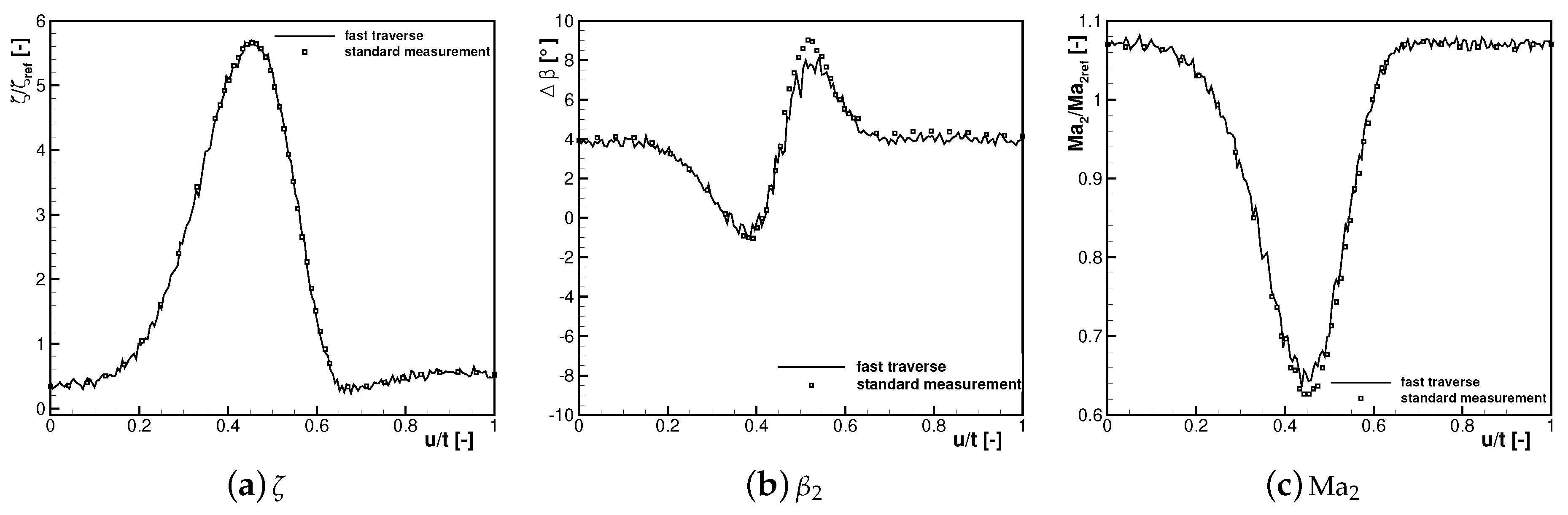
Doing so, the measurement accuracy for standard and new measurement techniques is 0.01 for the Mach number measured by the five-hole probe, $0.1^{\circ }$ for the swirl $\beta$ and approximately 10% of the total pressure loss coefficient $\zeta$ defined in Equation (20).

3. Test Set-Up

The experiments with a linear cascade were performed at the High-Speed Cascade Wind Tunnel of the Institute of Jet Propulsion at the Armed Forces University Munich. A drawing of the tunnel is given in Figure 3. The main components of the facility are a six-stage axial compressor, a settling chamber with laminar coolers and the nozzle. These parts are enclosed inside a pressure chamber where the static pressure can be changed between 3000 Pa and 120,000 Pa. Controlling the compressor speed and the cooling of the air, the flow Mach and Reynolds numbers (Ma and Re respectively) can be varied independently from each other. The Mach number range at the nozzle exit lies within $0.1\le \mathrm{Ma}\le 1$ and the range of the Reynolds number based on nozzle exit conditions divided by the geometric scale is approximately 2 ×${10}^5{\mathrm{m}}^{-1}$$\le \mathrm{Re}/l\le$ 16 ×${10}^6{\mathrm{m}}^{-1}$.

The compressor is driven by a 1.3 MW electric motor and the speed is controlled by a hydraulic coupling. These components are placed outside of the pressure chamber. Further details on the facility can be found in Sturm and Fottner [8].

3.1. Periodic Wake Generation

The interaction of the flow around the profile with periodically impinging wakes from an upstream moving airfoil can be simulated with cylindrical bars. The wake generator is placed at the nozzle exit and the cascade inside the wake generator. Cylindrical bars are moved linearly upstream of the cascade and parallel to it. After passing the circumferential end of the cascade, the bars do a ${180}^{\circ }$ turn and move backwards downstream of the cascade at sufficient distance not to interact with the outflow from the cascade. After a second turn, the cycle reinitializes. The wake generator was run at 40 m/s with a bar distance of 80 mm resulting in a frequency of 500 Hz of the wake disturbance. Details about the design can be found in Acton and Fottner [9].

3.2. Data Acquisition and Post Processing

The operating point of the cascade is controlled by the static pressure at the inlet to the cascade and the local stagnation pressure. The static pressure $p_1$ is measured with pressure taps at the sidewall of the nozzle, while the stagnation pressure $q_1$ is measured with a pitot probe in the nozzle. With these two pressures, the Mach number is computed assuming adiabatic isentropic expansion.

The Reynolds number is the second similarity parameter which is controlled using the definition

$$\mathrm{Re}=\sqrt{\frac{\gamma }{R}}\frac{c}{C_s}\frac{\mathrm{Ma}·p_1·\left(\frac{T_{t1}}{1+\left(\frac{\gamma -1}{2}\right)·{\mathrm{Ma}}^2}+S\right)}{{\left(\frac{T_{t1}}{1+\left(\frac{\gamma -1}{2}\right)·{\mathrm{Ma}}^2}\right)}^2}.$$

(19)

The total temperature of the flow $T_{t1}$ is measured with four PT100 resistance thermometers inside the settling chamber.

The downstream flow is measured with a five-hole pneumatic probe. The pressures at the five holes give the coefficients which allows to obtain the local Mach number ${\mathrm{Ma}}_2$, the local total pressure $p_{t2}$ and the flow angle in circumferential direction ${\beta }_2$. The total pressure is used to compute the profile losses defined by

$$\zeta =\frac{p_{t1}-p_{t2}}{q_1}.$$

(20)

Due to confidentiality reasons, the values are normalized by a random reference value or, in the case of the flow angle, given as difference from a reference value.

The integral values over one complete pitch are computed as mixed out values using the method of Amecke [10] where the conservation of mass, momentum and energy is fulfilled.

4. Experimental Results

The new method was applied on measurements downstream of a linear compressor cascade with moderate turning and a Mach number at the outlet of approximately 0.3. A broad range of Reynolds numbers were investigated but for briefness most of the results presented here are for two Reynolds numbers: a medium Reynolds number of 150,000 at which low profile loss is generated and a low Reynolds number of 50,000 where stalled flow is present. The method is shown to work also with periodically unsteady inflow.

Results from a traverse at the medium Reynolds number and steady inflow conditions are given in Figure 4. The normalized profile losses, the flow angle difference, and the normalized Mach number are given as a function of the relative pitchwise position. The results from a standard traverse are given as symbols and the ones from a fast traverse are drawn as lines. Each symbol of the standard traverse curve represents one of the 44 discrete measurement points. It is visible that, at these conditions, both measurements give very similar results along the pitch and all extreme values; gradients are also matched.

The results of the transient measurements shown here are for a traversing velocity of 2 mm/s. The same operating point was measured with a traversing velocity of 1 mm/s. In the latter case, the acquired pressures are closer to the actual values but after transformation with Equation (7) the results are similar for all three cases.

The method was also applied to measurements with unsteady inflow. Figure 5 depicts the flow properties downstream of the cascade for the same Reynolds number but with unsteady inflow. Furthermore, the differences are negligible. One should note that in Figure 5, the total pressure losses produced by the wake generator are included in the profile loss curve and that the scale of the ordinate was changed.

The difference in integral values between the standard and fast measurement technique is given in

Table 3. Differences of integral values using the standard and fast traverse technique

Flow Property	Steady Inflow	Unsteady Inflow
$\delta \zeta /\zeta$	0.044	0.0021
$\delta \beta$	$0.{01}^{\circ }$	$0.{01}^{\circ }$
$\delta \mathrm{Ma}$	0.001	0.001

. The differences are well below the measurement accuracy. The method described here therefore seems to be reliable.

More difficult to measure are operating points with very low Reynolds numbers due to the low absolute pressures. Nevertheless, the method gives decent results compared to the standard technique in Figure 6. Only the flow angle is computed considerably differently with an integral offset of $0.{25}^{\circ }$.

The measurement time decrease is depicted in Figure 7 for low and medium Reynolds number cases. The total time needed is normalized by the time needed at the low Reynolds number with the standard technique. One can see that the new technique can decrease the total time needed for one traverse by up to 90%. For a better estimate of the time saved, the typical overall measurement time for a standard traverse at low Reynolds number is approximately 45 min.

With the same technique, it is also possible to measure complete outflows from a cascade performing multiple traverses at different radial positions. The coefficients of the transfer function are only computed for the first traverse, since the measurement set-up and the overall pressure level remain constant for the other traverses. An insight into the quality of such measurements is given in Figure 8 where the measured total pressure loss along half span of the airfoil is depicted. The vectors are proportional to the secondary flow velocities. These results were acquired for an intermediate Reynolds number of ${\mathrm{Re}}_1$ = 75,000 at steady inflow conditions. The mid-span is located at $z/h=0$ and the sidewall at $z/h=0.5$. No whole plane measurements using the standard technique for comparison were performed due to the high time consumption, but at mid-span the results for both techniques are again similar. Nevertheless, the results of Figure 8 seem plausible with the correct picture of the secondary flow vortices.

The same technique was also applied to measurements downstream of a transonic turbine cascade and the results are similarly encouraging.

5. Conclusions

This paper presents a new method to measure the flow downstream of a cascade with a standard five-hole probe. The new method is based on obtaining a transfer function from two traverses with the direction of probe movement in opposite directions.

The technique presented here has been tested on compressor and turbine cascades and allows to decrease the total measurement time by up to 90% without noticeable loss in accuracy. In fact, due to a better spatial resolution of the flow, the accuracy can be increased for specific cases. The latter can be even more important when measuring complete outflow planes, where this technique was also applied successfully.

An extensive error analysis on measurements using a transfer function is performed. The analysis shows the way in which to obtain proper coefficients to reduce the measurement uncertainty. If no attention is paid to this, the uncertainty will grow exponentially with the increasing number of data points.

References

1. Grimshaw, S.; Taylor, J. Fast Settling Millimetre-Scale Five-Hole Probes. In Proceedings of the ASME Turbo Expo 2016: Turbomachinery Technical Conference and Exposition, Seoul, Korea, 13–17 June 2016. [Google Scholar]
2. Paniagua, G.; Dénos, R. Digital compensation of pressure sensors in the time domain. Exp. Fluids 2002, 32, 417–424. [Google Scholar] [CrossRef]
3. Sinclair, A.R.; Robins, A.W. A Method for the Determination of the Time Lag in Pressure Measuring Systems Incorporating Capillaries; NACA Technical Note 2793; National Advisory Committee for Aeronautics, Langley Aeronautical Lab: Langley Field, VA, USA, 1952. [Google Scholar]
4. Larcombe, M.; Peto, J. The Response Times of Typical Transducer-Tube Configurations for the Measurement of Pressures in High-Speed Wind Tunnels; Aeronautical Research Council Current Papers 913; Aeronautical Research Council, HM Stationery Office: London, UK, 1966. [Google Scholar]
5. Bartsch, C.; Hölle, M.; Jeschke, P.; Metzler, T. One-Dimensional Flow-Adaptive Measurement Grid Algorithm for Pneumatic Probe Measurements. J. Eng. Gas Turbines Power 2017, 138, 031601. [Google Scholar] [CrossRef]
6. Bergh, H.; Tijdeman, H. Theoretical and Experimental Results for the Dynamic Response of Pressure Measuring Systems; NLR-TR F.238; National Aerospace Laboratory (NLR): Amsterdam, The Netherlands, 1965. [Google Scholar]
7. Carolus, T. Kunststoffleitungen zwischen Druckmeßstelle und Druckaufnehmer als Fehlerquelle bei der Messung instationärer Drucksignale. Forsch. Ing. A 1986, 52, 191–197. [Google Scholar] [CrossRef]
8. Sturm, W.; Fottner, L. The High-Speed Cascade Wind-Tunnel of the German Armed Forces University Munich. In Proceedings of the 8th Sympsium on Measuring Techniques for Transonic and Supersonic Flows in Cascades and Turbomachines, Genoa, Italy, 24–25 October 1985. [Google Scholar]
9. Acton, P.; Fottner, L. The Generation of Instationary Flow Conditions in the High-Speed Cascade Wind Tunnel of the German Armed Forces University Munich. In Proceedings of the 13th Symposium on Measuring Techniques, Zürich, Switzerland, 5–6 September 1996. [Google Scholar]
10. Amecke, J. Auswertung von Nachlaufmessungen an ebenen Schaufelgittern; Technical Report 67 A 49; AVA: Göttingen, Germany, 1967. [Google Scholar]
Figure 1. Settling time as a function of the initial pressure p 0 .
Ijtpp 03 00006 g001
Figure 2. Measured pressure difference between total inlet pressure and centre bore of the probe normalized by stagnation pressure and resulting normalized pressure difference as an outcome of the transfer function. (a) Measured pressures; (b) Measured and reconstructed pressures.
Ijtpp 03 00006 g002
Figure 3. Drawing of the High-Speed Cascade Wind Tunnel.
Ijtpp 03 00006 g003
Figure 4. Flow properties measured downstream of the cascade with the standard and fast traverse technique for medium Reynolds number and steady inflow.
Ijtpp 03 00006 g004
Figure 5. Flow properties measured downstream of the cascade with the standard and fast traverse technique for medium Reynolds number and periodically unsteady inflow.
Ijtpp 03 00006 g005
Figure 6. Flow properties measured downstream of the cascade with the standard and fast traverse technique for low Reynolds number and periodically unsteady inflow.
Ijtpp 03 00006 g006
Figure 7. Total measurement time needed for a complete traverse.
Ijtpp 03 00006 g007
Figure 8. Normalized total pressure loss coefficient and secondary flow velocity vectors in a plane downstream of the cascade at Re 1 = 75,000 acquired with the fast technique.
Ijtpp 03 00006 g008