The Influence of Different Wake Profiles on Losses in a Low Pressure Turbine Cascade †


1
Engineering and the Environment, University of Southampton, Southampton SO17 1BJ, UK
2
Department of Mechanical Engineering, University of Melbourne, Melbourne 3010, Australia
*
Author to whom correspondence should be addressed.
†
This paper is an extended version of our paper published in Proceedings of the European Turbomachinery Conference ETC12 2017, Paper No. 213.
Int. J. Turbomach. Propuls. Power 2018, 3(2), 10; https://doi.org/10.3390/ijtpp3020010
Submission received: 14 December 2017
/
Revised: 21 March 2018
/
Accepted: 11 April 2018
/
Published: 17 April 2018
Abstract
:Large eddy simulations were carried out in order to investigate the influence of unsteady incoming wakes with different profiles on the loss mechanisms of the high lift T106Alinear low-pressure turbine (LPT) cascade. Bars placed upstream of the LPT blade were set into rotation around their axis, thus generating circulation, as well as asymmetrical wake profiles. Three different rotation rates were simulated, yielding different wake parameters that were then compared to an actual turbine blade wake profile. Whereas the commonly-used non-rotating bars generated wakes with turbulent kinetic energy levels several times higher than that of an actual blade wake, the case with counter-clockwise rotation led to more rapid wake mixing. All three wakes were able to trigger boundary layer transition and thus intermittently prevent separation on the suction surface. However, the weaker the wakes, the larger and longer lasting the separation bubbles became, and an increase in profile losses could be observed. Interestingly, the configuration with the weakest wake and the largest separation bubble resulted in a reduction of the overall LPT loss.
1. Introduction
The low-pressure turbine (LPT) in a jet engine makes up 20–30% of its total weight, and its dimension is restricted by the diameter of the jet engine casing. Furthermore, the rotational speed of the LPT and hence the prevalent flow velocities are determined by the operational range of the fan, which is driven by the turbine. Typical chord-based Reynolds numbers range from to [1].
In order to lower the operational cost of a jet engine, the weight of a turbine can be reduced by decreasing the blade count. As a consequence, each blade has to generate more lift and thus experiences a higher loading [1]. In the Reynolds number range in which an LPT operates, boundary layer transition and separation play an important role and have to be taken into account in the design process. Owing to the higher loadings, the boundary layer on the suction side of the blade is exposed to large adverse pressure gradients leading to unsteady transitional boundary layers [2]. Hodson and Howell [1] state that as the flow on the pressure side still accelerates in the direction of the trailing edge, the boundary layer remains laminar in most cases. A laminar separation bubble develops on the suction surface on the rear part of the blade due to the adverse pressure gradient. The separation bubble is highly sensitive to unsteady incoming wakes and disturbed flow in the LP turbine [1]. Thus, the boundary layer on the suction surface of the blade is the main focus when considering two-dimensional profile losses.
In order to simplify both experiments and simulations, a setup with moving bars upstream of the rotor is commonly used to generate velocity wakes [3,4,5,6], which are also referred to as ‘negative jets’ as they pass over the blades [7]. In an extensive study, Halstead et al. [8] exposed three forms of boundary layer transition on blades in a turbine cascade caused by incoming wakes. Schulte and Hodson [9] found in their experimental investigations that wakes impinging on the blade increase the wall shear stress and thus create more losses. They also ascertained that the incoming wakes can prevent laminar separation and the development of a separation bubble due to the induction of early transition. This means that, since the size of the separation bubble is related to the loss of efficiency [10], wakes can reduce the overall loss compared to cases without wakes. The effect is stronger for highly loaded blades, where a large separation bubble is present in steady cases without incoming wakes.
Michelassi et al. [11] demonstrated the importance of the reduced frequencies and flow coefficients in their large eddy simulations (LES) of a linear low-pressure turbine cascade. The degree of wake mixing before the leading edge determined how distinct the wakes are that enter the blade passage. More distinct wakes caused a more unsteady boundary layer, whereas mixed out wakes resulted in a more free-stream turbulence-like behaviour. Halstead et al. [12] found that wakes with higher turbulent kinetic energy move the transition point upstream. Between wake passings, the calming effect (where a non-turbulent boundary layer appears after the occurrence of turbulent spots induced by the wakes) was also stronger resulting in transition locations further downstream compared to the weaker wake case. Recently, LES simulations on a linear turbine stage with two different gap sizes were conducted by Pichler et al. [13]. In the smaller gap configuration, having stronger wakes passing through the rotor stage, a separation bubble could be prevented, which led to a slightly lower profile loss.
Understanding these complex mechanisms is vital in order to further increase the efficiency and to reduce the operational costs, by allowing even higher blade loadings, of a jet engine. Thus, wakes have become an important part of the design process of low pressure turbine blades and are used as a means of flow control [9]. The aim of this work is to investigate the effect of wakes that are more similar to actual blade wakes in terms of intensity and width than wakes generated by upstream bars that are moving in the pitch-wise direction only. In order to do so, the well-known Magnus effect is exploited by setting the bars into rotation around their axis [14]. The influence on the loss mechanisms of the cascade is then investigated.
2. Methods
Simulations of the linear low-pressure turbine have been conducted using the in-house solver HiPSTAR. The compressible Navier–Stokes equations for an ideal gas are solved on multi-block structured curvilinear grids. Prior to the simulations, a transformation of the Navier–Stokes equations from a coordinate system to a generalised coordinate system is performed. However, only the streamwise (axial) and pitch-wise coordinates are mapped, which allows for an independent spanwise grid and thus reduces the memory consumption [2].
The streamwise and lateral directions are discretised by a fourth-order accurate compact finite difference scheme [15]. By applying a skew-symmetric splitting approach to the non-linear terms of the governing equations, the numerical stability is increased [16]. The discretisation of the spanwise direction, which is assumed to be uniformly spaced and periodic, is done by a Fourier transformation using the FFTW library [17]. Time advancement is performed by a five-step fourth-order Runge–Kutta scheme introduced by Kennedy et al. [18].
Prior to this work, the code had been validated by comparing the direct numerical simulations (DNS) results [2] of the high lift T106A linear low-pressure turbine cascade with measurements of Stadtmüller [19]. Furthermore, LES simulations, conducted in an extensive study by Michelassi et al. [11], of the same setup were validated against the DNS results. The wall-adapting local eddy-viscosity (WALE) sub-grid model of Nicoud and Ducros [20] was used, which was also employed within this study.
Soft inflow and non-reflecting outflow boundary conditions based on Kim and Lee [21] were chosen. The block interfaces of the multi-block setup were connected by the characteristic interface conditions of Kim and Lee [22]. In order to establish a relative motion between the wake-generating bars upstream and the turbine blade, sliding interface conditions, proposed by Johnstone et al. [23], between the first four blocks were applied (see Figure 1). An immersed boundary approach, namely the boundary data immersion method (BDIM) [24], was used for the representation of the bars. This provided the flexibility to alter the bar position and geometry, as well as the use of a simple Cartesian grid. The BDIM had been validated for aero-vibro-acoustic DNS simulations [25] prior to this study.
2.1. Grid
The grid was generated with a multi-block Poisson grid generator for cascade simulations [26] and is similar to the one that was already used in the previously conducted LES study of Michelassi et al. [11]. The setup and domain decomposition of the linear low-pressure turbine with two wake-generating bars is shown in Figure 1. Periodic boundary conditions for the pitch-wise and spanwise directions were applied. The two bars are located 0.7 true chord-lengths, c, upstream of the blade’s leading edge () with a bar pitch of . Based on the size of the round trailing edge of the turbine blade, the bar diameters were set to . In order to achieve a relative motion between the bars and the blade, the two upstream blocks are connected to the cascade grid via the aforementioned sliding interface.
The whole 3D grid for the large eddy simulations amounts to 12 million grid points, with 32 Fourier modes, or 66 collocation points, for the spanwise discretisation and grid points in the 2D plane. With a distance of for the first grid point from the blade surface, a value of is achieved. However, in the aft region of the blade where flow transition and separation occurs, drops well below 1, ensuring DNS-like resolution.
2.2. Simulations
The chosen flow parameters including the inlet velocities, Mach and Reynolds numbers for all simulations are shown in Table 1. The resulting isentropic Reynolds and Mach numbers, which are defined based on the exit velocity at (denoted ‘Measurement Plane 2’ in Figure 1) and the true chord length c, are around and , respectively. In order to fully describe the compressible Navier–Stokes equations with the ideal gas assumption, the Prandtl number and the Sutherland constant S are also given in the table.
There are two important parameters that determine the state of the incoming wakes. First is the flow coefficient:
with the axial flow velocity and the bar sliding velocity . Second is the reduced frequency:
These parameters were chosen because the study of Michelassi et al. [11] found that for configurations with a bar count of two or less, distinct wakes enter the cascade passage without mixing out beforehand. Additionally, with the two bar setup less, simulation time is required for gathering time and phase-lock averaged statistical data owing to the higher wake passing frequency. Given these parameters, an equivalent background turbulence, due to the wake mixing within the blade passage, of was obtained.
In order to establish wakes with different intensities and thus representing different gap sizes, the bars rotate around their axis with three different rotation rates:
The rotation rate is defined by the angular velocity , the bar diameter D and the free stream velocity . In the following, the cases are denoted by , and . denotes the non-rotating bar setup, which is commonly used in the experimental and numerical works throughout the literature. The bars in the cases and rotate in the counter-clockwise and clockwise direction with a tangential velocity of , respectively. Counter-clockwise rotating bars correspond more closely to the LPT configuration, creating a lift force, owing to the Magnus effect, that points in the opposing direction relative to the blade. The clockwise rotation setup was chosen in order to provide a range of wake properties. Additionally, a setup without upstream bars was simulated.
3. Results
Both time and phase-locked averaged statistics were gathered in order to investigate the flow field. All simulations were restarted based on an initial simulation and then run for more than 15 non-dimensional time units in order to go past the transient. One non-dimensional time unit, t, corresponds to the time it takes for the flow with unit velocity to convect over one chord length, c. After that, data over another 16 non-dimensional time units were collected for the averaged statistics. The periodicity in the spanwise direction allowed for a spatial averaging in this direction while the simulation was running, reducing the costs for I/O. Lastly, the already spatially averaged data were then averaged over time.
For the phase-locked averaging, each bar passing period, defined by:
with the bar count , was divided into 24 phases, and each phase was then averaged over 16 bar passing periods T.
In the following, the results are divided into two parts. Firstly, the different bar wake profiles are investigated and compared to an actual blade wake. Secondly, the implications of the different wakes on the blade profile and the turbine losses are presented.
3.1. Wake Results
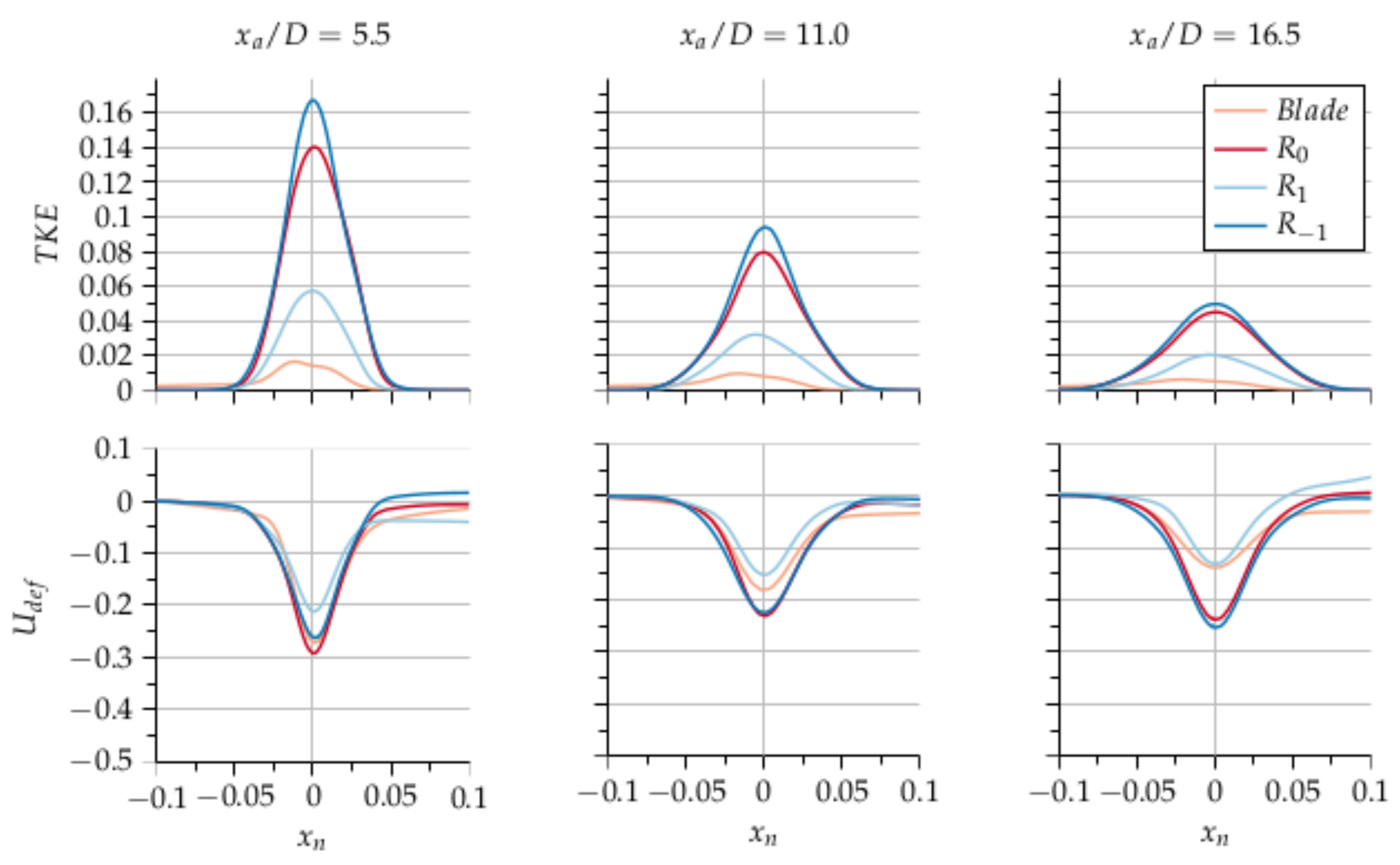
The differences between the bar wakes and the actual blade wake are first shown by means of time-averaged statistics. In order to do so, wake profile data perpendicular to the wake centre lines at three different positions , and , based on the bar diameter D, downstream of the bars and blade were extracted. The centre lines were determined by the peak velocity deficit locations in the wakes.
The turbulent kinetic energy, (top) and the velocity deficit, (bottom) profiles for the three different positions are shown in Figure 2. These quantities were normalised by and , respectively, with the local velocity, obtained outside of the wakes. A fairly rapid mixing of all the wakes, indicated by the decreasing and widening of the profiles while moving downstream, is evident. The clockwise rotating bars generate wakes with the highest levels of turbulent kinetic energy, followed by the stationary bar case. Slightly skewed and much weaker wake profiles are achieved by the counter-clockwise rotating bars, which are more similar in shape to an actual blade wake. However, the turbulent kinetic energy is a factor of three higher. The fact that the bars generate much higher levels of turbulent kinetic energy is in agreement with the experimental findings of Halstead et al. [8] (p. 442).
The velocity deficits of the bar wake profiles, aligned at point , for the cases and are quite similar for all three downstream positions. In the case, the amplitude of the velocity deficit is markedly lower and decays in a similar manner to the blade wake. Interestingly, the profiles of the bar wakes compare better to the blade wake profiles, as opposed to the profiles.
Owing to the different rotation rates of the upstream bars, the flow turning is changed, altering the angle of attack , obtained at Measurement Position 1. However, it is important to maintain the angle of attack, for the blade constant for all the cases in order to be able to attribute the effects on the turbine caused by the different wakes only. By changing the pitch-wise flow velocity, , at the inlet plane and keeping the streamwise component, , unaltered, which would influence the mass flow rate and the flow coefficient (Equation (1)) otherwise, the flow turning can be compensated. Table 2 shows the flow correction angle that was needed in order to compensate the flow turning and establish a constant angle of attack . This also ensured that the same turbine conditions, determined by the isentropic Reynolds, and Mach numbers, , could be achieved. Hence, the differences shown in the Results Section can be solely attributed to the different bar wake properties. As can be seen, the correction only has a small effect on the bar Reynolds number, .
Furthermore, the drag, , and lift, , coefficients parallel and perpendicular to the flow direction, respectively, are given. Owing to the Magnus effect, different values were obtained, which allows one to check whether the drag coefficient is a reliable parameter as a design criterion for bars, as stated by Pfeil and Eifler [27]. The mixed out losses, (see Equation (6) for definition), behind the bars () show a strong correlation with the drag coefficients.
Phase-locked averaged results enable the tracking of the wakes passing through the cascade at different time instants. As already mentioned, one bar passing period was divided into 24 phases, which were averaged over a total of 16 periods.
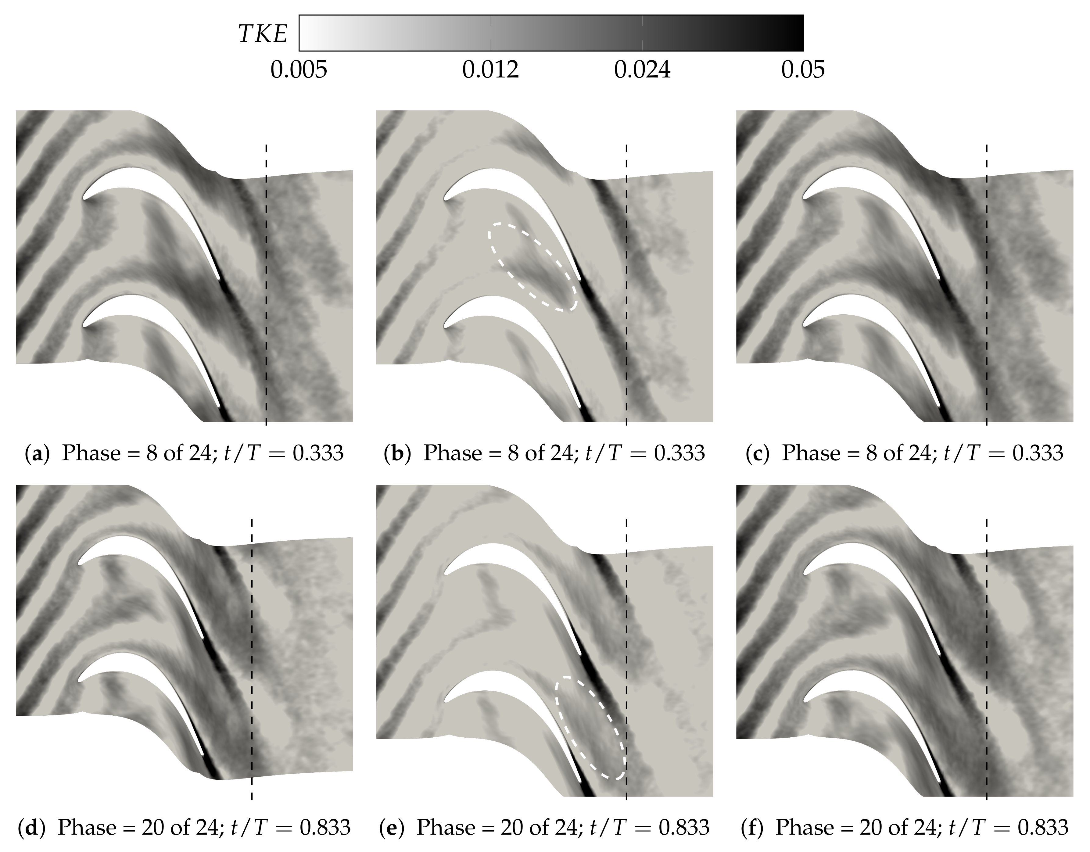
The phase-lock averaged turbulent kinetic energy, , for the three different bar wakes at two different phases is shown in Figure 3. As can be seen, the wakes of the cases (a,d) and (c,f) passing through the turbine passage are much more pronounced than the wake of case (b,e). The typical wake distortion, as described by Smith [28], and an increase in turbulent kinetic energy in the passing wake close to the suction surface, as observed by other authors [29,30], were apparent for all cases. Furthermore, the levels of of the blade wakes are substantially higher compared to the bar wakes, but finally merge with them further downstream.
3.2. Implications for the Turbine Cascade
The state of the blade wakes is dependent on the state of the boundary layers, which in turn are influenced by the bar wakes passing through the blade passage. A mutual dependence between the bar wakes and the blade wakes is the result, which will be investigated more deeply in the following sections. In order to do so, firstly, the influence of the bar wakes on the blade itself is presented. After that, the combined effects of the merged blade and bar wakes in terms of loss quantification are examined.
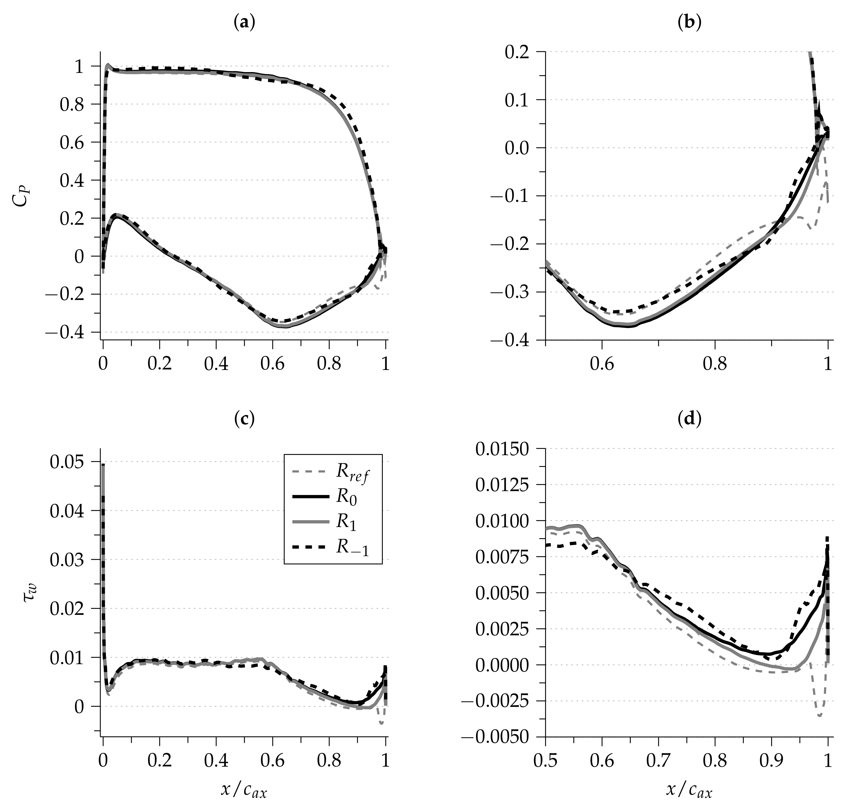
Time-averaged plots of the pressure coefficient over the whole blade surface and the wall shear stress on the suction surface are shown in Figure 4a,c. For all cases, there are virtually no differences in for most of the blade surface. The portion most affected by the bar wakes is restricted to the aft region of the suction surface of the blade. The strongest wakes, case , slightly increase the pressure on both the suction and the pressure surface compared to the other cases. A separation bubble for the case, which starts at around and reattaches near , can be observed (Figure 4b,d). The reference case shows a marked difference from up to the trailing edge, indicating an even larger separation bubble.
The wall shear stress, , on the suction surface is identical for cases and up to . After that point, drops for and goes below zero, but then rapidly recovers. The wall shear stress for the case drops at around and then increases at , yielding the highest values. These differences correlate with the strength of the bar wakes, where the strongest wakes produce the highest due to the mixing with the turbulent boundary layer in the aft portion, whereas the weakest wakes are not able to prevent the separation bubble. Furthermore, the wall shear stress level for the reference case is marginally lower from the leading edge up to . Towards the trailing edge, is significantly lower compared to the cases with bars, leading to a large separation bubble. This large separation bubble decreases the peak velocity on the blade and hence results in the mentioned reduction of before . The latter bubble, indicated by a sharp dip in wall shear stress, closes again at the trailing edge. The kink in the and slopes is caused by an additional small separation region behind the trailing edge.
Figure 5 shows the velocity contours, the edge of the boundary layer (black dashed) and the displacement thickness, (white dashed), on the suction surface of the turbine blade. For that, the tangential flow velocity was extracted as a function of the wall normal direction. Due to the pronounced wake regions in the boundary layer profiles, the first derivative of the tangential velocity in the wall normal direction, , was used to determine the boundary layer edge. The position where the derivative is minimal or crosses a given value denotes the edge of the boundary layer.
The most striking feature that can be observed is the length of the separation bubble for the reference case and its wall-normal extension into the blade passage. The boundary layer remains laminar until the top of the bubble, then transitions and closes the separation shortly before the trailing edge. The cases and show very similar contours. A small separation bubble for case can be observed, as well. The most apparent differences can be observed in the thickening of the displacement thickness for cases and due to the separation bubbles.
Phase-locked averaged data are used in order to further investigate the effects on the cascade blade. A space-time diagram of the wall shear stress on the suction surface along the blade surface s, normalised by the total suction surface length S, for three bar passing periods is shown in Figure 6. Additionally, the time-averaged free stream velocities are plotted on top of the contours, where the peak velocity is aligned with the peak spot at around . The white spots denote wall shear stress levels below zero, i.e., flow separation. Qualitatively, the cases with bars are fairly similar for the majority of the blade, as already observed for the time-averaged results. The wall shear stress levels on the mid-chord, where the wakes hit the blade surface, seem to be slightly lower for case . This is consistent with the experimental results of Halstead et al. [8], who found increasing levels of wall shear stress for stronger wakes impinging on the blade. However, as already observed in Figure 4, the wakes in case cause slightly lower stress levels compared to case in the mid-chord region.
Looking at the aft section of the blade, a large separation bubble for most of the time period can be observed for . The size, the start and end point, as well as the duration of the bubbles markedly vary over the bar passing periods. At some time instants, two distinct separation bubbles occur. In the case of , the size and the duration of the bubbles are substantially reduced. For case , the separation bubbles are almost completely suppressed. Owing to the absence of incoming wakes, the reference case does not show much variation over time, although there is clearly unsteadiness. Looking at a highly resolved time signal close to the bubble, the frequency and period of this unsteadiness could be calculated, yielding and , respectively. The values correspond to the vortex shedding frequency at the trailing edge and do not necessarily correlate with the frequencies of the instabilities that eventually lead to transition, as was also found by Wheeler et al. [31], although for a high-pressure turbine blade.
The reason for the larger separation bubble for case can be explained by looking at the incoming wakes passing through the blade passage; see Figure 3. Due to the sensitivity of the separated flow to inflow disturbances, like incoming wakes, the weaker wakes of the case seem to be less effective at reducing the size of the bubble, whereas the wakes for case , which have the highest levels, are most effective. As can be seen, this results in larger calmed regions, yielding a reduced separation bubble. This is also consistent with the experimental results of Halstead et al. [8] and the simulation results of Sarkar [32].
As the size of the separation bubble is related to the loss generation [10], the largest loss values are to be expected from the reference case , whereas the resulting loss values for the bar cases depend on both the incoming wakes and the size of the separation bubble. Furthermore, time varying losses for all cases should be linked to unsteadiness, which was even observed for the case without bars.
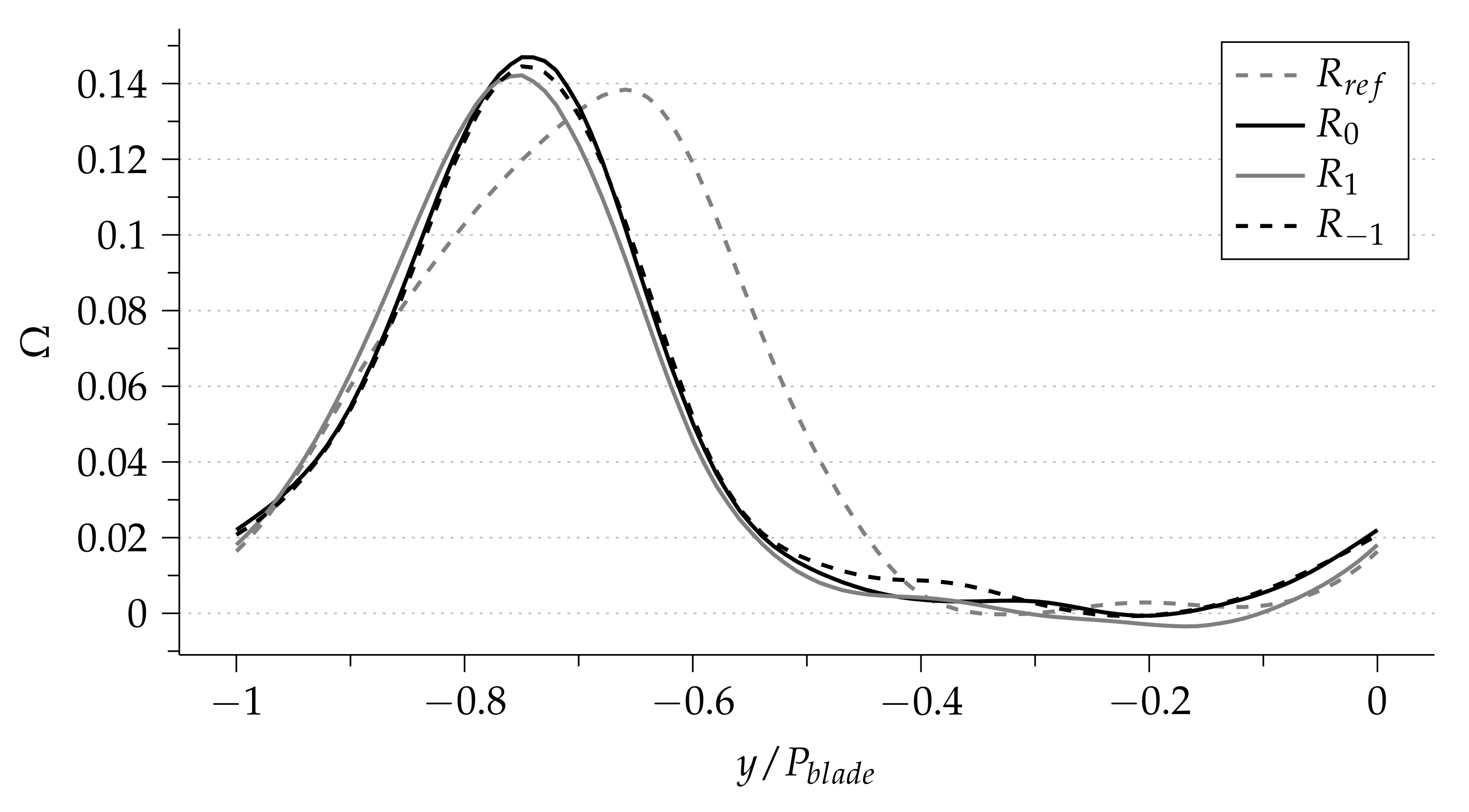
The losses in a low-pressure turbine cascade can be quantified by the total pressure loss , where is the mass averaged total pressure calculated at ‘Measurement Plane 1’, is the mass averaged static pressure at ‘Measurement Plane 2’ and is the total pressure profile at ‘Measurement Plane 2’. Loss profiles for all cases are shown in Figure 7. The profile peaks, denoting the total pressure loss due to the blade wake, of and are very similar. The slightly lower peak loss value might be explained by the smaller separation bubble, only observed in the phase-lock averaging, for case . For the bar case with the largest separation bubble, , the peak loss value is the lowest, and the blade wake is slightly shifted, as well. The lowest peak loss, however, can be observed for the reference case without incoming bars. A significant deflection and widening of the blade wake is the result of the large separation bubble.
The losses in the region of the profile away from the peak values can be attributed to the passing wakes or rather to the losses generated in the turbine passage. At around , the losses are most elevated for case with the clockwise rotating bars, which produced the most pronounced wakes and hence had the strongest wake distortion. For case , with the weakest incoming bar wakes, the smallest amount of pressure loss in the blade passage can be seen. The negative loss between is due to varying inlet values in the pitch-wise direction caused by the bars [33].
Denton [34] identified three sources accounting for the overall profile loss, which will be referred to as Denton loss (D) in the following;
The first term of the right-hand side is the base pressure loss (A) consisting of the base pressure coefficient and the displacement thickness, , at the trailing edge with thickness . The losses due to the momentum and the displacement thickness at the trailing edge are given by the second (B) and the third (C) term, respectively. Another value to quantify losses in turbines is the mixed-out loss (E) [35], defined by:
see Figure 1 identifying Measurement Planes 1 and 2. Rather than mass averaging, the flow variables are irreversibly mixed out to a state of complete equilibrium. The Indices 1 and 2 denote Measurement Planes 1 and 2 in Figure 1, respectively. The Denton losses () and their respective terms, the overall mixed-out losses (E) and the wake distortion losses (F), where only the part of the profile outside the blade boundary layer is taken into account, are shown in Figure 8. For the latter, only values less than roughly of the peak total pressure loss of the respective profile were considered.
There are no apparent differences in the base pressure losses, A, for the three bar cases. The same observation can be made for the losses due to the momentum thickness, B. Owing to the larger separation bubble and hence a larger displacement thickness for case , the displacement loss, C, due to blockage effects, is increased, leading to a higher overall Denton loss, D, compared to the other cases. For the reference case, a negative base pressure was obtained due to a small second separation region behind the trailing edge. Furthermore, the momentum loss is lower compared to the bar cases. The very large separation bubble causes a marked increase for the displacement loss; however, a significantly lower overall Denton loss is achieved.
The highest mixed out loss, E, is produced in the reference case , as was already expected due to the large separation bubble. The bar case , which led to the largest bubble, generated the lowest loss, whereas for case with the almost non-existent separation bubble, the highest loss out of the three bar cases is obtained. Another reason for this can be found by looking at the wake distortion losses F. As can be seen, the wakes with the lowest levels, as well as the lowest drag coefficient and mixed out loss (Table 2, in case ) also produce the least loss as opposed to the case with the most pronounced wakes, . The production term, defined by:
explains this behaviour, as already pointed out by Stieger and Hodson [30]. The higher the turbulent stresses , as is the case for , the higher the production of turbulent kinetic energy and hence an increase in wake distortion losses. A comparison between the Denton losses, D, and the mixed out losses, E, in combination with the wake distortion losses, F, reveals the importance of wake mixing effects. The Denton loss decreases for decreasing sizes of the separation bubble, but due to the stronger wakes, which in turn are responsible for the shrinkage of the separated region, the overall losses increase. Here, the reference case represents a special case, where due to the strong widening of the blade wake, the highest overall mixed out loss is achieved, but the lowest profile loss.
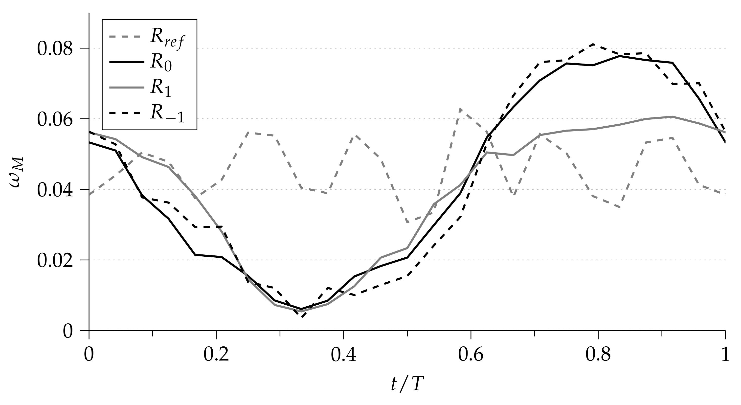
The phase-lock averaged mixed-out losses for one bar passing period are presented in Figure 9. A distinct minimum and maximum peak loss for all bar cases are evident. Furthermore, all bar cases reach a similar minimum loss at around . Considering the contours in Figure 3a–c (the black dashed line denotes the loss accounting plane) and the space-time diagram (Figure 6) for , it is clear that the minimum loss occurs at the time without a separation bubble on the blades and when the bar wake has not mixed with the blade wake yet. The opposite effect can be seen from onwards, where a separation bubble occurs, for all cases, and the bar wakes mix with the blade wake. Lower losses are generated in the case, whereas cases and reach a similar maximum loss. The deviation between the cases from to can be attributed to the influence of the larger separation bubble in the bar case. This again demonstrates that the absence or reduction of a separation bubble in a low-pressure turbine does not necessarily lead to reduced overall losses, since wake distortion and the combined effects play an important role.
As already expected from the space-time diagram in Figure 6, the reference case shows an unsteady loss behaviour, as well, with a period related to the vortex shedding frequency of the blade, but has a smaller amplitude due to the absence of the bar wakes. Hence, in this case, the time varying mixed-out losses can be solely attributed to the large separation bubble and the vortex shedding at the trailing edge.
In conclusion, the interaction between the weaker incoming wakes in case and the blade wake leads to considerably lower overall and maximum losses, even though a much larger separation bubble is present, leading to higher profile losses. The consideration of the levels is important when choosing wake-generating bars in the design process. This can be realised by using rotating bars and changing the drag coefficient, as already stated by Pfeil and Eifler [27]; it has been proven to be a viable alternative to using different bar diameters. The very different lift coefficients did not contribute to any observable effect in our simulations.
As mentioned, the reduced frequency was chosen such that distinct wakes enter the blade passage. For higher reduced frequencies, the strength of the wakes might no longer be as important, as wake mixing occurs before the blade’s leading edge [11]. Moreover, added inlet turbulence and higher Reynolds numbers can positively affect the losses [6], and hence, the importance of the wake strength might change, as well. Coull et al. [36] have shown that for higher Reynolds numbers, the wakes dominate the profile loss generation due to the increase of the momentum thickness of the turbulent boundary layer.
4. Conclusions
Large eddy simulations of the T106A linear low-pressure turbine cascade were carried out. Three different bar wakes, generated by means of different bar rotation rates, and a blade wake were investigated. By setting the wake-generating bars into rotation, it was possible to achieve more similar wakes compared to an actual blade wake in terms of wake width. It has been shown that the levels of the wakes for the non-rotating bars, which are commonly used, are several times higher compared to a turbine blade wake. In the experimental study of Halstead et al. [8], who used different bar diameters, the authors came to the same conclusion.
The effect of the three different bar wake profiles on the loss mechanisms of the low-pressure turbine was also considered, as incoming wakes have a profound effect on the profile losses [37]. Mean pressure and wall shear stress profiles of the blade differed only in the rear part of the blade’s suction surface, where a separation bubble could be observed in the case with the weakest incoming wakes. A space-time diagram of the wall shear stress on the suction surface revealed a markedly bigger and longer-lasting separation bubble per blade passing period for . For case , with clockwise rotation, the bubble could almost be completely prevented. A reason for the larger separation bubble is due to the weaker wake boundary-layer interaction and thus the positive effects of earlier transition and calmed regions are less pronounced. It was also shown that the maximum and overall loss was lower for the clockwise rotating bar case, even though a larger and longer-lasting separation bubble was present. Both mechanisms, the strength of the incoming wakes and the size of the separation bubble, and the combined effect on the overall loss generation have to be considered in the design process. Hence, it is paramount to choose a bar setup that generates reasonable wakes in terms of levels.
Acknowledgments
The simulations have been carried out on the supercomputer of the U.K. National Supercomputing Service ARCHER. Resources were provided by the U.K. Turbulence Consortium funded by the EPSRC under Grant Number EP/L000261/1. Furthermore, the authors gratefully acknowledge the Supercomputing facility of the University of Southampton. Richard D. Sandberg acknowledges the financial support by veski.
Author Contributions
Florian Hammer carried out the large eddy simulations. All authors contributed to the discussion of the results.
Conflicts of Interest
The authors declare no conflict of interest.
Abbreviations
The following abbreviations are used in this manuscript:
| Acronyms | |
| I/O | Input/Output |
| DNS | Direct numerical simulation |
| LES | Large eddy simulations |
| LPT | Low-pressure turbinet |
| NS | Navier–Stokes |
| Nomenclature | |
| c | true chord length |
| axial chord length | |
| , , | drag and lift coefficient |
| , | pressure and base pressure coefficient |
| reduced frequency | |
| turbulent kinetic energy | |
| M | Mach number |
| p | static pressure |
| stagnation pressure | |
| bar pitch | |
| blade pitch | |
| Prandtl number | |
| Reynolds number | |
| S | Sutherland constant, total suction surface length |
| t | dimensionless time unit |
| T | blade passing frequency |
| reference temperature | |
| tangential velocity | |
| reference velocity | |
| bar velocity | |
| velocity deficit | |
| axial flow velocity | |
| pitch-wise flow velocity | |
| axis along the wakes | |
| axis normal to the wakes | |
| Greek | |
| rotation rate | |
| blade inflow angle | |
| blade outflow angle | |
| displacement thickness | |
| normal to flow direction | |
| flow coefficient | |
| wall shear stress | |
| momentum thickness | |
| mixed-out loss | |
| total pressure loss | |
| parallel to flow direction | |
| Subscripts | |
| inflow plane | |
| outflow plane | |
| axial direction | |
| mixed-out quantity | |
| pitch-wise direction | |
| reference value | |
| stagnation value | |
| at trailing edge |
References
- Hodson, H.P.; Howell, R.J. The role of transition in high-lift low-pressure turbines for aeroengines. Prog. Aerosp. Sci. 2005, 41, 419–454. [Google Scholar] [CrossRef]
- Sandberg, R.D.; Pichler, R.; Chen, L.; Johnstone, R.; Michelassi, V. Compressible Direct Numerical Simulation of Low-Pressure Turbines: Part I—Methodology. J. Turbomach. 2015, 137, 051011. [Google Scholar] [CrossRef]
- Ladwig, M.; Fottner, L. Experimental Investigations of the Influence of Incoming Wakes on the Losses of a Linear Turbine Cascade. In Proceedings of the ASME 1993 International Gas Turbine and Aeroengine Congress and Exposition, Cincinnati, OH, USA, 24–27 May 1993; p. V03CT17A055. [Google Scholar]
- Engber, M.; Fottner, L. The Effect of Incoming Wakes in Boundary Layer Transition. In Loss Mechanisms and Unsteady Flows in Turbomachines; Advisory Group fpr Aerospace Research and Development, North Atlantic Treaty Organization: Neuilly sur Seine, France, 1996. [Google Scholar]
- Wu, X.; Jacobs, R.G.; Hunt, J.C.R.; Durbin, P.A. Simulation of boundary layer transition induced by periodically passing wakes. J. Fluid Mech. 1999, 398, 109–153. [Google Scholar] [CrossRef]
- Michelassi, V.; Chen, L.; Pichler, R.; Sandberg, R.D. Compressible Direct Numerical Simulation of Low-Pressure Turbines: Part II—Effect of Inflow Disturbances. J. Turbomach. 2015, 137, 071005. [Google Scholar] [CrossRef]
- Meyer, R.X. The Effect of Wakes on the Transient Pressure and Velocity Distributions in Turbomachines. ASME J. Basic Eng. 1958, 80, 1544–1552. [Google Scholar]
- Halstead, D.E.; Wisler, D.C.; Okiishi, T.H.; Walker, G.J.; Hodson, H.P.; Shin, H.W. Boundary Layer Development in Axial Compressors and Turbines: Part 3 of 4—LP Turbines. J. Turbomach. 1997, 119, 225–237. [Google Scholar] [CrossRef]
- Schulte, V.; Hodson, H.P. Unsteady Wake-Induced Boundary Layer Transition in High Lift LP Turbines. J. Turbomach. 1998, 120, 28. [Google Scholar] [CrossRef]
- Coull, J.D.; Hodson, H.P. Unsteady boundary-layer transition in low-pressure turbines. J. Fluid Mech. 2011, 681, 370–410. [Google Scholar] [CrossRef]
- Michelassi, V.; Chen, L.W.; Pichler, R.; Sandberg, R.; Bhaskaran, R. High-Fidelity Simulations of Low-Pressure Turbines: Effect of Flow Coefficient and Reduced Frequency on Losses. J. Turbomach. 2016, 138, 111006. [Google Scholar] [CrossRef]
- Halstead, D.E.; Wisler, D.C.; Okiishi, T.H.; Walker, G.J.; Hodson, H.P.; Shin, H.W. Boundary Layer Development in Axial Compressors and Turbines: Part 2 of 4—Compressors. J. Turbomach. 1997, 119, 426–444. [Google Scholar] [CrossRef]
- Pichler, R.; Michelassi, V.; Sandberg, R.; Ong, J. Highly Resolved Large Eddy Simulation Study of Gap Size Effect on Low-Pressure Turbine Stage. J. Turbomach. 2017, 140, 021003. [Google Scholar] [CrossRef]
- Prandtl, L. Magnuseffekt und Windkraftschiff. Sci. Nat. 1925, 13, 93–108. [Google Scholar] [CrossRef]
- Kim, J.W.; Sandberg, R.D. Efficient parallel computing with a compact finite difference scheme. Comput. Fluids 2012, 58, 70–87. [Google Scholar] [CrossRef]
- Kennedy, C.A.; Gruber, A. Reduced aliasing formulations of the convective terms within the Navier–Stokes equations for a compressible fluid. J. Comput. Phys. 2008, 227, 1676–1700. [Google Scholar] [CrossRef]
- Frigo, M.; Johnson, S.G. The design and implementation of FFTW3. Proc. IEEE 2005, 93, 216–231. [Google Scholar] [CrossRef]
- Kennedy, C.A.; Carpenter, M.H.; Lewis, R.M. Low-storage, explicit Runge–Kutta schemes for the compressible Navier–Stokes equations. Appl. Numer. Math. 2000, 35, 177–219. [Google Scholar] [CrossRef]
- Stadtmüller, P. Investigation of Wake-Induced Transition on the LP Turbine Cascade T106A-EIZ, DFG-Verbundprojekt Fo 136 11, Version 1.0; Universität der Bundeswehr München: Munich, Germany, 2001. [Google Scholar]
- Nicoud, F.; Ducros, F. Subgrid-Scale Stress Modelling Based on the Square of the Velocity Gradient Tensor. Flow Turbul. Combust. 1999, 62, 183–200. [Google Scholar] [CrossRef]
- Kim, J.W.; Lee, D.J. Generalized characteristic boundary conditions for computational aeroacoustics. AIAA J. 2000, 38, 2040–2049. [Google Scholar] [CrossRef]
- Kim, J.W.; Lee, D.J. Characteristic interface conditions for multi-block high-order computation on singular structured grid. AIAA J. 2003, 41, 2341–2348. [Google Scholar] [CrossRef]
- Johnstone, R.; Chen, L.; Sandberg, R.D. A sliding characteristic interface condition for direct numerical simulations. Comput. Fluids 2015, 107, 165–177. [Google Scholar] [CrossRef]
- Weymouth, G.D.; Yue, D.K.P. Boundary data immersion method for Cartesian-grid simulations of fluid-body interaction problems. J. Computat. Phys. 2011, 230, 6233–6247. [Google Scholar] [CrossRef]
- Schlanderer, S.C.; Weymouth, G.D.; Sandberg, R.D. The boundary data immersion method for compressible flows with application to aeroacoustics. J. Comput. Phys. 2017, 333, 440–461. [Google Scholar] [CrossRef]
- Gross, A.; Fasel, H.F. Multi-block Poisson grid generator for cascade simulations. Math. Comput. Simul. 2008, 79, 416–428. [Google Scholar] [CrossRef]
- Pfeil, H.; Eifler, J. Turbulenzverhältnisse hinter rotierenden Zylindergittern. J. Forsch. Ing-Wes. 1976, 42, 27–32. [Google Scholar] [CrossRef]
- Smith, L.H. Wake Dispersion in Turbomachines. J. Basic Eng. 1966, 88, 688–690. [Google Scholar] [CrossRef]
- Michelassi, V.; Wissink, J.G.; Rodi, W. DNS, LES and URANS of Periodic Unsteady Flow in a LP Turbine Cascade: A Comparison. Proc. Inst. Mech. Eng. Part A J. Power Energy 2003, 217, 403–411. [Google Scholar] [CrossRef]
- Stieger, R.D.; Hodson, H.P. The Unsteady Development of a Turbulent Wake Through a Downstream Low-Pressure Turbine Blade Passage. J. Turbomach. 2005, 127, 388–394. [Google Scholar] [CrossRef]
- Wheeler, A.P.S.; Sandberg, R.D.; Sandham, N.D.; Pichler, R.; Michelassi, V.; Laskowski, G. Direct Numerical Simulations of a High-Pressure Turbine Vane. J. Turbomach. 2016, 138, 071003. [Google Scholar] [CrossRef]
- Sarkar, S. Influence of Wake Structure on Unsteady Flow in a Low Pressure Turbine Blade Passage. J. Turbomach. 2009, 131, 041016. [Google Scholar] [CrossRef]
- Leggett, J.; Priebe, S.; Shabbir, A.; Sandberg, R.; Richardson, E.; Michelassi, V. LES loss prediction in an axial compressor cascade at off-design incidences with free stream disturbances. In Proceedings of the ASME Turbo Expo 2017: Turbomachinery Technical Conference and Exposition Turbomachinery, Charlotte, NC, USA, 26–30 June 2017; p. V02AT39A031. [Google Scholar]
- Denton, J.D. The 1993 IGTI Scholar Lecture: Loss Mechanisms in Turbomachines. J. Turbomach. 1993, 115, 621–656. [Google Scholar] [CrossRef]
- Prasad, A. Calculation of the Mixed-Out State in Turbomachine Flows. J. Turbomach. 2005, 127, 564–572. [Google Scholar] [CrossRef]
- Coull, J.D.; Thomas, R.L.; Hodson, H.P. Velocity Distributions for Low Pressure Turbines. J. Turbomach. 2010, 132, 041006. [Google Scholar] [CrossRef]
- Hodson, H.P.; Howell, R.J. Bladerow Interactions, Transition, and High-Lift Aerofoils in Low-Pressure Turbines. Annu. Rev. Fluid Mech. 2005, 37, 71–98. [Google Scholar] [CrossRef]
Figure 1.
Setup of the linear low-pressure turbine with two wake-generating bars upstream.
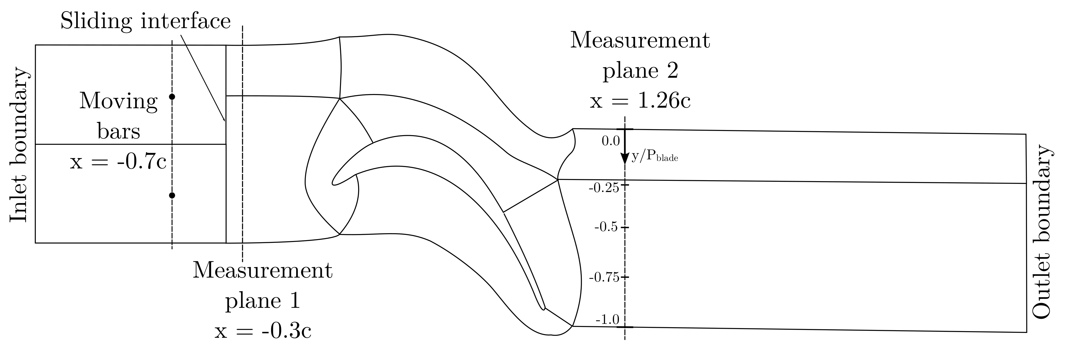
Figure 2.
Comparison of the normalised turbulent kinetic energy (top) and the velocity deficit (bottom) of the bar and blade wakes for different downstream positions. and denote the axes parallel and perpendicular to the wakes, respectively. The non-rotating bar case is denoted by , the counter-clockwise rotating bar case by , the clockwise rotating bar case by and the wake off a low pressure turbine (LPT) blade by Blade.

Figure 3.
Phase-lock averaged turbulent kinetic energy () at different phases for the non-rotating bar case (a,d), the counter-clockwise rotating bar case (b,e) and the clockwise rotating bar case (c,f).
Figure 3.
Phase-lock averaged turbulent kinetic energy () at different phases for the non-rotating bar case (a,d), the counter-clockwise rotating bar case (b,e) and the clockwise rotating bar case (c,f).

Figure 4.
Comparison of the time-averaged pressure coefficient (a,b) and the wall shear stress (c,d) for the four cases. With the non-rotating bar case , the counter-clockwise rotating bar case , the clockwise rotating bar case and the reference case without bars.
Figure 4.
Comparison of the time-averaged pressure coefficient (a,b) and the wall shear stress (c,d) for the four cases. With the non-rotating bar case , the counter-clockwise rotating bar case , the clockwise rotating bar case and the reference case without bars.

Figure 5.
Velocity contours, edge of the boundary layer (black dashed line) and displacement thickness, , (white dashed line) along the suction surface for the non-rotating bar case , the counter-clockwise rotating bar case , the clockwise rotating bar case and the reference case without bars.
Figure 5.
Velocity contours, edge of the boundary layer (black dashed line) and displacement thickness, , (white dashed line) along the suction surface for the non-rotating bar case , the counter-clockwise rotating bar case , the clockwise rotating bar case and the reference case without bars.
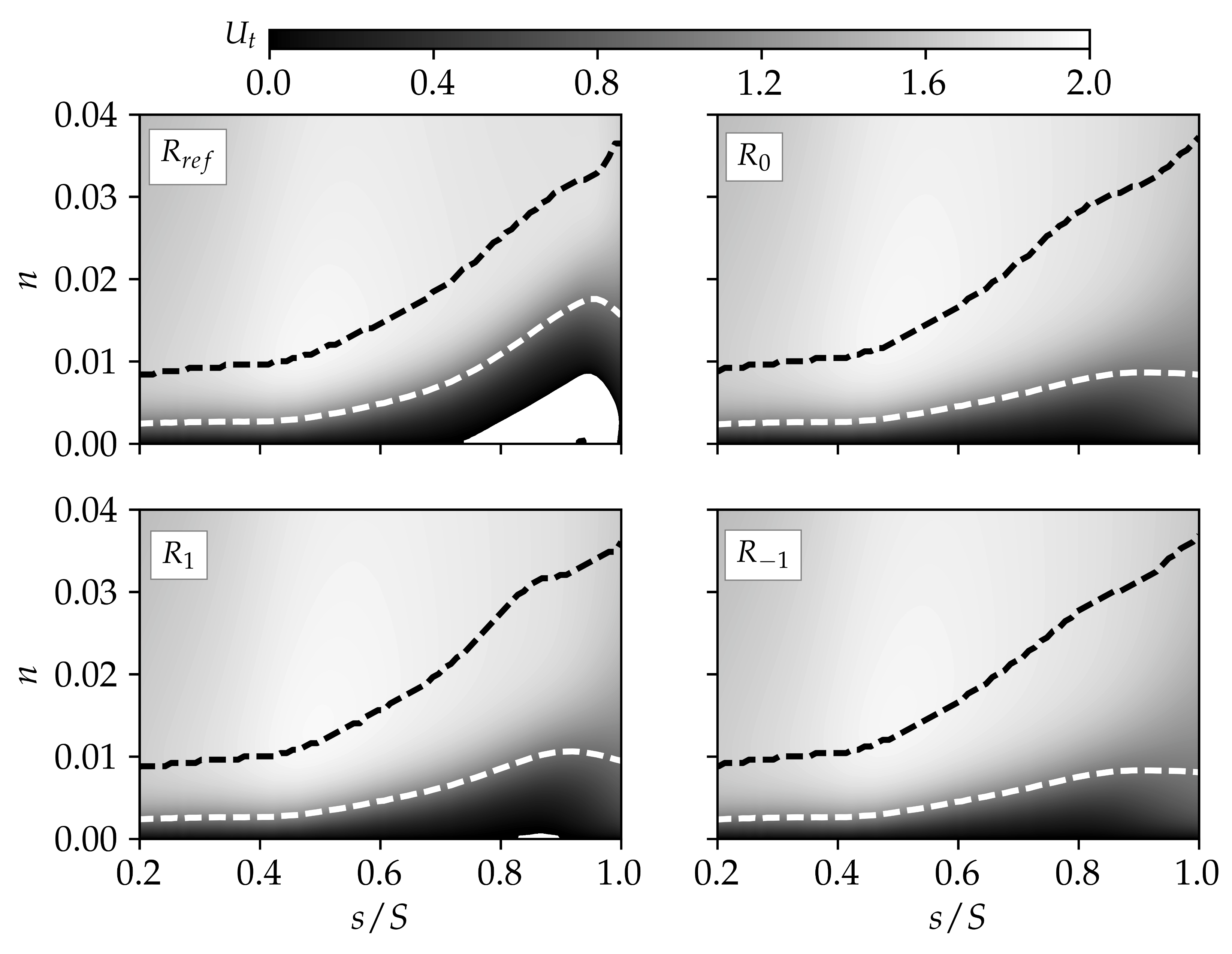
Figure 6.
Space-time diagram of the suction side wall shear stress along the streamwise direction for three bar passing periods, for cases (no bars), (counter-clockwise), (non-rotating) and (clockwise).
Figure 6.
Space-time diagram of the suction side wall shear stress along the streamwise direction for three bar passing periods, for cases (no bars), (counter-clockwise), (non-rotating) and (clockwise).
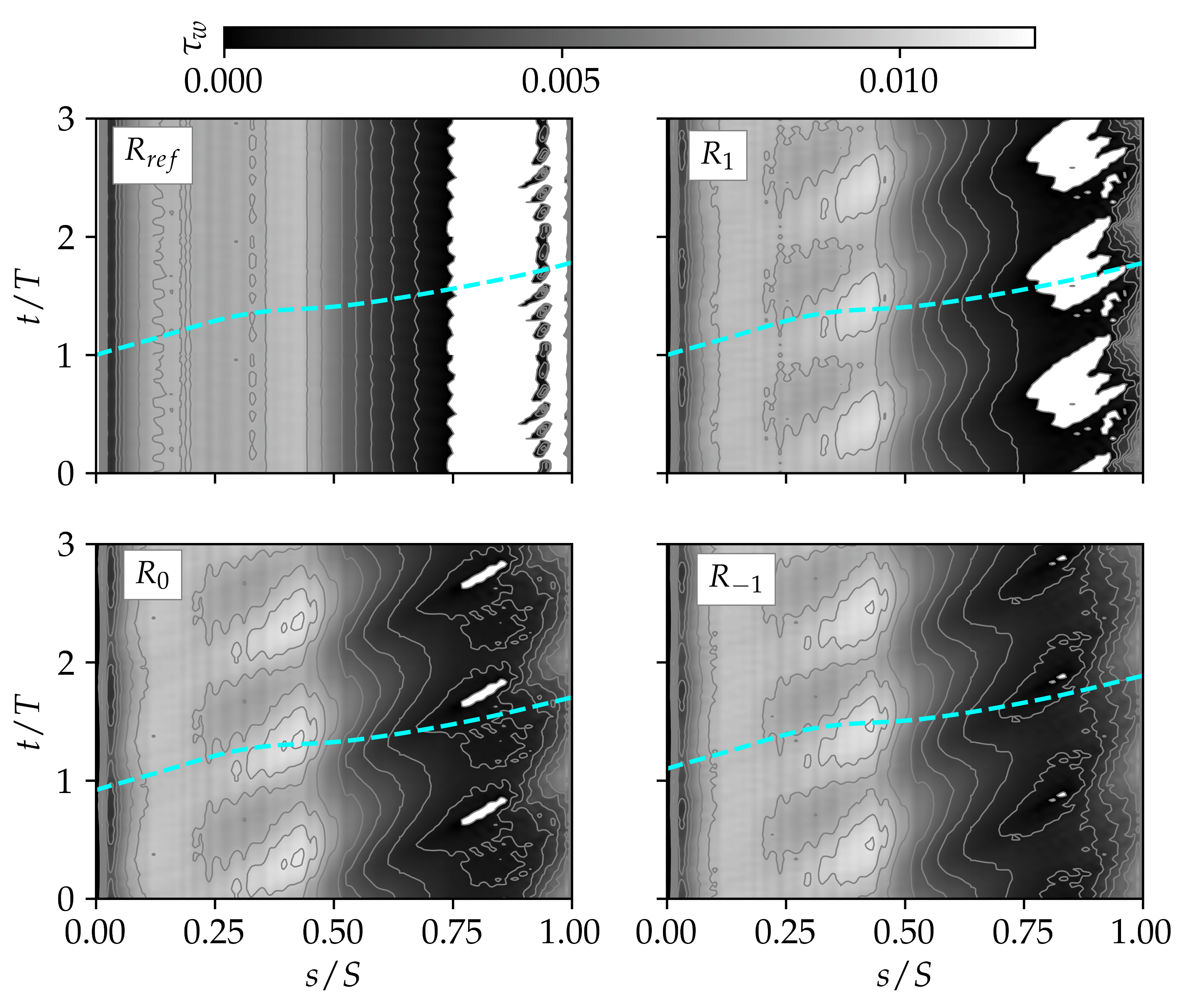
Figure 7.
Time-averaged total pressure loss profile extracted at ‘Measurement Plane 2’ () for cases (no bars), (counter-clockwise), (non-rotating) and (clockwise).
Figure 7.
Time-averaged total pressure loss profile extracted at ‘Measurement Plane 2’ () for cases (no bars), (counter-clockwise), (non-rotating) and (clockwise).

Figure 8.
Denton losses (A–D), overall mixed-out losses (E) and wake distortion losses (F).
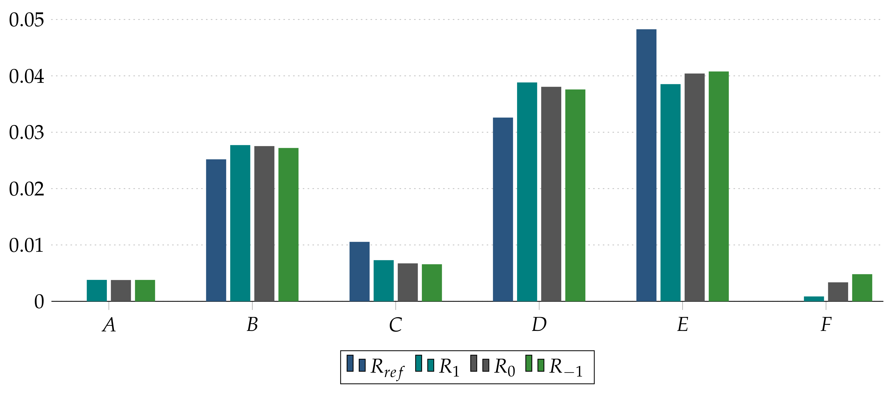
Figure 9.
The variation of the mixed-out losses for one bar passing period.

Table 1.
Inlet parameters for the cascade simulations.
| M | |||||
|---|---|---|---|---|---|
| 62,707 | 0.24357 | 0.697 | 0.41 | 0.72 | 0.3686 |
Reynolds number, ; Mach number, M; axial velocity, ; bar velocity, ; Prandtl number, ; Sutherland constant, S.
Table 2.
Resulting low-pressure turbine flow conditions.
| ≈98,000 | 0.4074 | - | 43.04 | 40.00 | - | - | 0.0001 | |
| ≈98,000 | 0.4059 | 1663 | 42.91 | 46.05 | 1.5503 | −0.0914 | 0.1317 | |
| ≈98,000 | 0.4074 | 1714 | 42.64 | 37.45 | 0.9307 | −2.8347 | 0.0748 | |
| ≈98,000 | 0.4053 | 1545 | 42.76 | 50.15 | 1.6730 | 1.6400 | 0.1434 |
Isentropic Reynolds number, ; isentropic Mach number, ; bar Reynolds number, ; angle of attack, ; flow correction angle, , at the domain inlet; drag, , and lift, , coefficients; mixed out loss, .
© 2018 by the authors. Licensee MDPI, Basel, Switzerland. This article is an open access article distributed under the terms and conditions of the Creative Commons Attribution (CC BY-NC-ND) license (https://creativecommons.org/licenses/by-nc-nd/4.0/).
Share and Cite
MDPI and ACS Style
Hammer, F.; Sandham, N.D.; Sandberg, R.D. The Influence of Different Wake Profiles on Losses in a Low Pressure Turbine Cascade. Int. J. Turbomach. Propuls. Power 2018, 3, 10. https://doi.org/10.3390/ijtpp3020010
AMA Style
Hammer F, Sandham ND, Sandberg RD. The Influence of Different Wake Profiles on Losses in a Low Pressure Turbine Cascade. International Journal of Turbomachinery, Propulsion and Power. 2018; 3(2):10. https://doi.org/10.3390/ijtpp3020010
Chicago/Turabian StyleHammer, Florian, Neil D. Sandham, and Richard D. Sandberg. 2018. "The Influence of Different Wake Profiles on Losses in a Low Pressure Turbine Cascade" International Journal of Turbomachinery, Propulsion and Power 3, no. 2: 10. https://doi.org/10.3390/ijtpp3020010