The Kernel of the Distributed Order Fractional Derivatives with an Application to Complex Materials


1
College of Geoscience, Texas A & M University, College Station, TX 77843, USA
2
Department of Mathematics, University of Bologna, Piazza Porta San Donato 5, 40129 Bologna, Italy
*
Author to whom correspondence should be addressed.
Fractal Fract. 2017, 1(1), 13; https://doi.org/10.3390/fractalfract1010013
Submission received: 24 October 2017
/
Revised: 13 November 2017
/
Accepted: 13 November 2017
/
Published: 21 November 2017
(This article belongs to the Special Issue Fractional Dynamics)
Abstract
:The extension of the fractional order derivative to the distributed order fractional derivative (DOFD) is somewhat simple from a formal point of view, but it does not yet have a simple, obvious analytic form that allows its fast numerical calculation, which is necessary when solving differential equations with DOFD. In this paper, we supply a simple analytic kernel for the Caputo DOFD and the Caputo-Fabrizio DOFD, which may be used for numerical calculation in cases where the weight function is unity. This, in turn, could potentially allow faster solution of differential equations containing DOFD. Utilizing an analytical formulation of simple physical systems with phenomenological equations that include a DOFD, we show the relevant differences between the Caputo DOFD and the Caputo-Fabrizio DOFD. Finally, we propose a model based on DOFD for modeling composed materials that comprise different constituents, and show its compatibility with thermodynamics.
1. Introduction
The distributed order fractional derivative (DOFD) was introduced in 1967 [1] and, rightly, received no attention from the scientific community, since the simpler derivative of fractional order was being successfully used in several different fields of science, such as as a filter for studying spectral properties, in diffusion, and in Maxwell equations [2,3]; Bagley and Torvik, in [4], developed a theory to show the existence of the order domain and the solution of distributed order equations.
Then, interest slowly increased, with several interesting papers being published; of particular note among them are Chechkin et al. [5], who applied DOFD to study retarding subdiffusion and accelerating superdiffusion; Lorenzo and Hartley [6], who studied variable-order and distributed-order fractional operators; Chechkin et al. [7] applied distributed-order time-fractional operators in the fractional equations; Naber [8] studied distributed-order fractional subdiffusion; Kochubei [9] applied distributed-order operators to the study of ultraslow diffusion; and Mainardi et al. [10] applied DOFD to study the diffusion.
Recently, Jiao et al. [11] treated the problems of stability, simulation, applications and perspectives of dynamic systems modeled with the use of this new operator, and Gorenflo et al. [12] (see also [13]) found a fundamental solution of a distributed order time-fractional diffusion equations.
The original definition of the fractional derivative of distributed order includes cases where the derivative is affected by a weight function, which adds more difficulties to those that already exist in the numerical computation of the derivative, including that of the computer time required for its numerical estimation. In any case, in this work, we have observed that the DOFD is reduced to a classical operator with a kernel.
The purpose of this short article is to give an analytic expression for the DOFD in the case of unity weight function, which, with the use of a simple convolution with a given transfer function, may contribute to obtaining a faster numerical computation and more rapid solution of equations.
Moreover, it is convenient to note that the use of DOFD allows the expansion of memory operator applications to new materials.
Indeed, in the last section, we consider a model for which the distributed-order fraction derivative is used to represent constitutive equations describing the behavior of composite materials realized from multiple physical constituents, such that the mesoscopic structure of some materials can be considered as a set of sample materials, which we assume to be represented by materials that can be described by a fractional derivative. Therefore, such composite materials can be represented by assembling the singular components by a fractional derivative of a distributed order. Moreover, we prove that these composed materials satisfy the Thermodynamic Principles, from which we obtain the existence of free energy for the system.
2. The Caputo DOFD
The Laplace Transform (LT) of (1), exchanging the operator of LT with that of integration [4], is
Here, z, with the dimension of time, is a normalization parameter used for the consistency of the physical dimensions [3]. For purposes of formal simplification, we assume z = 1 in the following, which does not limit our discussion.
In practice, it is often the case that one assumes A(v) = 1, which gives
Setting
we may write
or
where we consider h(t) to be a pseudo-Green function of the problem when A(v) = 1 or the kernel of Caputo DOFD.
LTh(t) = H(s)
In the following, we find the time domain expression of h(t) appearing in Equations (5) and (6) required for the computation of .
We find first the following properties for H(s)
which imply,
That is, the Caputo DOFD has a singularity in the origin.
In the following, we find the time domain expression of h(t) appearing in Equations (5) and (6) required for the computation of by integrating along the Bromwich-Hankel path
or finally
which is a pseudo-Green function of the DOFD order with a unity weight function.
Equation (6) implies that
which is the explicit closed-form expression for the DOFD with a unity weight function.
Dividing the numerator and denominator of the integrand in Equation (9) by rd, we find
which implies that by increasing d, the integrand decreases; or that by interpreting d as a normalized distance from the origin of the signal and the sensor, the signal decreases with increasing distance d. In other words we have a model of decreasing signal with increases in both time and distance.
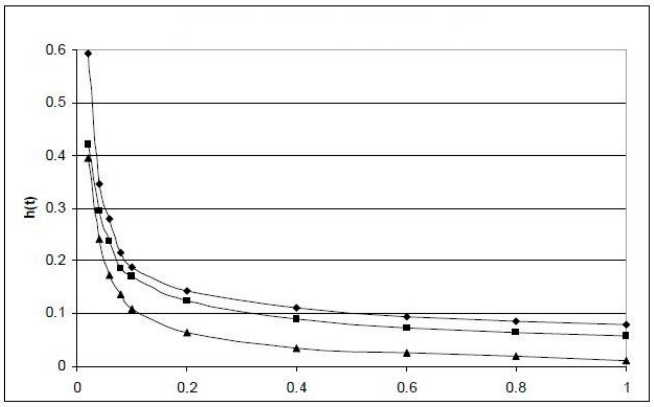
The time domain expression of the pseudo-Green function h(t) is shown graphically in Figure 1 with c = 0.8; d = 0.9; with c = 0.45; d = 0.55 and with c = 0.1; d = 0.2.
It may be useful to see the analytic form of the DOFD of some elementary functions often seen in the literature. We consider the functions f(t) = cos kt, f(t) = exp(−at) and f(t) = t; finding respectively
and
It is obvious that the of a constant is nil.
The may be used in phenomenological equations for natural phenomena in order to model memory. However, at this point, it is legitimate to ask about the differences between their filtering performance and that of the simpler Dvw(t), as well as asking which one would be more convenient, since both may be estimated numerically with roughly equal efficiency.
For a tentative comparison, we consider the very simple case of an input-output system with memory alternatively represented by the Dvw(t) and the . Simply put, the has two free parameters, c and d, while the Dvw(t) has only v as a free parameter; this is the major formal difference. In our case, because of the apparent complexity of both the problem and, possibly, of its solution, we tentatively chose to use .
3. Application to an Input-Output System with Memory Constitutive Equation
Let g(t) be the output and w(t) the input, and assume that they are related by
where G(s) = LTg(t) and W(s) = LTw(t), and a and b are arbitrary constants.
In the case of elasticity, Equation (13) would be the stress–strain relation of the generalized Kelvin Voigt type with g(t) strain and w(t) stress and a, b = gr cm−1 s−2; in the case of electric phenomena, w(t) would be the applied electric field and g(t) the induction.
With W = 1—that is, w(t) = δ(t) in Equation (14)—we find the pseudo-Green function
To compute g(t), we first see that the integral around s = 0 is nil, since 0 < c < d < 1, and then integrate around the Bromwich-Hankel path finding.
In accordance with the extreme value theorem, it can also be seen that .
With W = 1/s and Equation (14), we find the response to a constant stress
With w = sin(ft) in (14), we find the response to a periodic stress
4. The Caputo-Fabrizio DOFD
The Laplace Transform (LT) of (1), exchanging the operator of Laplace Transform with that of integration [4], is
In practice, it is often the case that one assumes A(s) = 1, which gives
Setting
we may write
where we consider h(t) a pseudo-Green function for the computation of the Caputo-Fabrizio DOFD with A(v) = 1 or, in other words, h(t) may be considered the kernel of the Caputo-Fabrizio DOFD. The time domain expression of the pseudo-Green function or kernel h(t) is shown graphically in Figure 2.
LTh(t) = H(s)
In the following, we find the time domain expression of h(t) appearing in Equations (27) and (28) required for the computation of the by integrating along the path of the complex plane with s = r exp(iθ) and setting θ = 3π/2 and θ = π/2, which is integrated over the interval [-∞, ∞] of the imaginary axis
which is a pseudo-Green function of Caputo-Fabrizio DOFD with unity weight function or its kernel.
Equation (29) implies that
which is the explicit closed-form expression for the Caputo-Fabrizio DOFD with unity weight function.
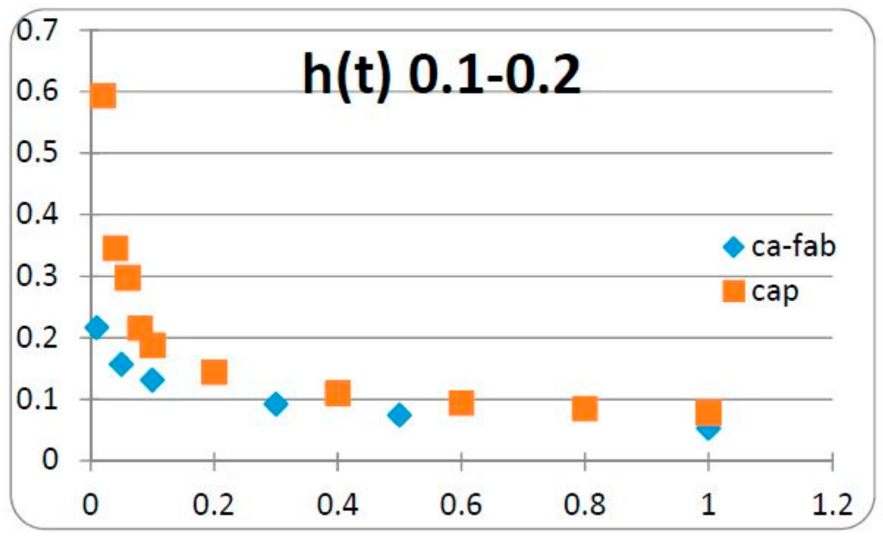
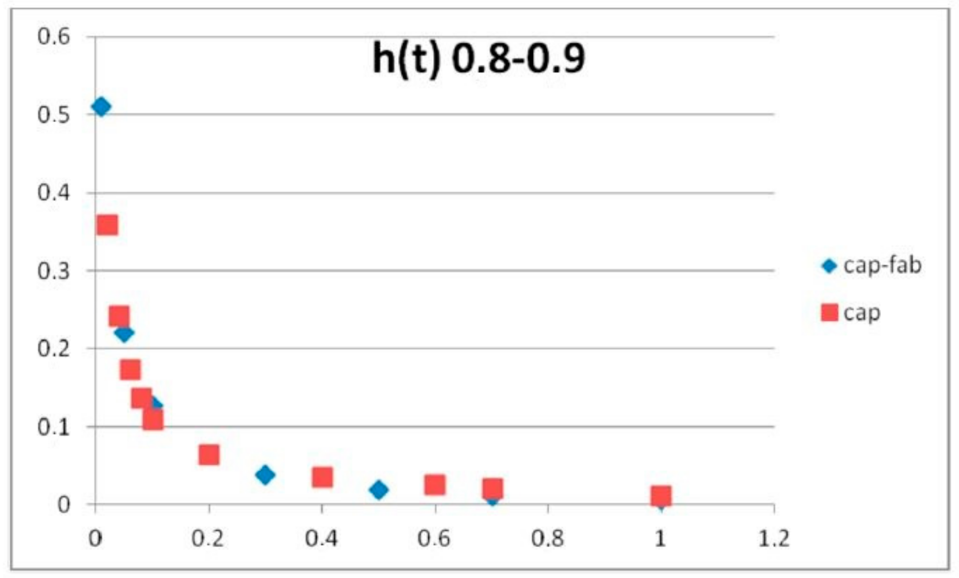
A comparison between the kernels of the Caputo DOFD and of Caputo-Fabrizio DOFD in the ranges 0.1–0.2, 0.45–0.55 and 0.8–0.9, as shown in the Figure 3, Figure 4 and Figure 5, indicates that, for values of the narrow intervals closer to unity, the two DOFDs are almost identical, which is not the case when the interval is close to zero.
5. Composite Materials by a DOFD
In this last section, we consider an application of DOFD for describing composite materials, fitting together a variety of constituents with different proprieties. When they are combined by a distributed fractional derivative, we obtain a material with new properties, compared to the single components. Specifically, in this paper, we consider composite systems (see Jones [15]), Schwartz [16]), and Vinson et al. [17]) whose constituents are materials with fading memory, which we represent with a fractional derivative such that the stress components are defined by the following constitutive equation
with the strain
where the vector u denotes the displacement.
So, for composite materials, we have the stress T(x,t) being defined by distributed-order fractional derivative , where
with C(x, t), a fourth order symmetric and positive tensor, and
from which
then
where
therefore, Equation (28) provides a classic memory relationship whose kernel is given by Equation (29).
Now, we study the case for which the stress components Tv are defined by the Caputo-Fabrizio fractional derivative [13]
Therefore, the stress tensor by the new fractional derivative in Equation (30) is given by
So that the kernel F(x, t − s) in Equation (28) is defined by
Then, for such a solid material, the differential problem on a smooth domain is given by
where ρ(x) is the density and f(x, t) the body forces.
Finally, following [10], we study the thermodynamic conditions related to the constitutive Equation (30) for which the state s is given by the history
σ(t) := ɛ(t − s)
Dissipation Principle
There exists a state function ψ(σ(t)) called free energy, for which the following inequality holds:
It is well known that, for a viscoelastic material, we have the following restriction from Inequality (32) (see [17])
for any ω > 0 and vectors .
So that, if w = (t − s), we have
from which, for any
Finally when we use the Caputo-Fabrizio fractional derivative (30), from Dissipation Principle (32) we have
6. Conclusions
In the 3 cases considered and illustrated in Figure 3, Figure 4 and Figure 5, the values of the kernels of the Caputo DOFD and of the Caputo-Fabrizio DOFD are compared. These values decrease monotonically by less than 0.1 at unit time; however, the Caputo DOFD diverges at t = 0, while the Caputo-Fabrizio DOFD is initially bounded, which has obvious implications, which need to be taken into account when selecting the most appropriate fractional derivative for the problem under consideration. So, when the fractional derivative is substituted by a distributed-order derivative, we may obtain the constitutive equation of a material with new properties compared to those given by the singular components.
Acknowledgments
This work was supported by the GNFM (Gruppo Nazionale di Fisica Matematica) of Italian CNR.
Author Contributions
From an initial idea of Michele Caputo, the paper was realized in complete collaboration. Both authors have read and approved the final manuscript.
Conflicts of Interest
The authors declare no conflict of interest.
References
- Caputo, M. Linear model of Dissipation whose Q is almost Frequency Independent-II. Geophys. J. Int. 1967, 13, 529–539. [Google Scholar] [CrossRef]
- Caputo, M. Mean Fractional-Order-Derivatives Differential Equations and Filters; Annali Università Ferrara: Ferrara, Italy, 1995; Volume 41, pp. 73–83. [Google Scholar]
- Caputo, M. Distributed order differential equations modelling dielectric induction and diffusion. Fract. Calc. Appl. Anal. 2001, 4, 421–442. [Google Scholar]
- Bagley, R.L.; Torvik, P.J. On the existence of the order domain and the solution of distributed order equations—Part I. Int. J. Appl. Math. 2000, 2, 865–882. [Google Scholar]
- Chechkin, A.V.; Gorenflo, R.; Sokolov, I.M. Retarding subdiffusion and accelerating superdiffusion governed by distributed-order fractional diffusion equations. Phys. Rev. E 2002, 66, 046129. [Google Scholar] [CrossRef] [PubMed]
- Lorenzo, C.F.; Hartley, T.T. Variable order and distributed order fractional operators. Nonlinear Dyn. 2002, 29, 1–4, 57–98. [Google Scholar] [CrossRef]
- Chechkin, A.V.; Gorenflo, R.; Sokolov, I.M. Distributed order time fractional diffusion equation. Fract. Calc. Appl. Anal. 2003. [Google Scholar] [CrossRef]
- Naber, M. Distributed order fractional sub-diffusion. Fractals 2004, 12, 23. [Google Scholar] [CrossRef]
- Kochubei, A.N. Distributed order calculus and equations of ultraslow diffusion. J. Math. Anal. Appl. 2008, 340, 257–281. [Google Scholar] [CrossRef]
- Mainardi, F.; Mura, A.; Pagnini, G. Time-fractional diffusion of distributed order. J. Vib. Control 2008, 14, 1267–1290. [Google Scholar] [CrossRef]
- Jiao, Z.; Chen, Y.Q.; Podlubny, I. Distributed-Order Dynamic Systems Stability, Simulation, Applications and Perspectives; Springer: Berlin, Germany, 2012. [Google Scholar]
- Gorenflo, R.; Luchko, Y.; Stojanovic, M. Fundamental solution of a distributed order time-fractional diffusion-wave equations as probability density. Fract. Calc. Appl. Anal. 2013, 16, 297–316. [Google Scholar] [CrossRef]
- Yang, X.J.; Baleanu, D.; Srivastava, H.M. Local Fractional Integral Transforms and Their Applications, 1st ed.; Academic Press: Cambridge, UK, 2015. [Google Scholar]
- Caputo, M.; Fabrizio, M. A new definition of fractional derivative without singular kernel. Progr. Fract. Differ. Appl. 2015, 1, 73–85. [Google Scholar]
- Jones, F.R. (Ed.) Handbook of Polymer-Fiber Composites; Longman Scientific and Technical: Essex, UK, 1994. [Google Scholar]
- Schwartz, M.M. Composite Materials Handbook; McGraw-Hill: New York, NY, USA, 1984. [Google Scholar]
- Vinson, J.R.; Sierakowski, R.L. The Behavior of Structures Composed of Composite Materials; Martinus Nighoff Publishers: Dordrecht, The Netherlands, 1986. [Google Scholar]
- Fabrizio, M. Fractional rheological models for thermomechanical systems. Dissipation and free energies. Fract. Calc. Appl. Anal. 2014, 17, 206–223. [Google Scholar]
- Fabrizio, M.; Giorgi, C.; Morro, A. Minimum principles, convexity, and thermodynamics in viscoelasticity. Contin. Mech. Thermodyn. 1989, 1, 197–211. [Google Scholar] [CrossRef]
Figure 1.
The form of the pseudo-Green function h(t) of the Caputo DOFD for different values of the couple (c, d) c = 0.8 ; d = 0.9 (triangles), c = 0.45; d = 0.55 (squares), c = 0.1; d = 0.2 (diamonds).
Figure 1.
The form of the pseudo-Green function h(t) of the Caputo DOFD for different values of the couple (c, d) c = 0.8 ; d = 0.9 (triangles), c = 0.45; d = 0.55 (squares), c = 0.1; d = 0.2 (diamonds).

Figure 2.
The time domain expression of the pseudo-Green function or kernel h(t) is shown graphically in the figure, with c = 0.8; d = 0.9; with c = 0.45; d = 0.55 and with c = 0.1; d = 0.2.
Figure 2.
The time domain expression of the pseudo-Green function or kernel h(t) is shown graphically in the figure, with c = 0.8; d = 0.9; with c = 0.45; d = 0.55 and with c = 0.1; d = 0.2.
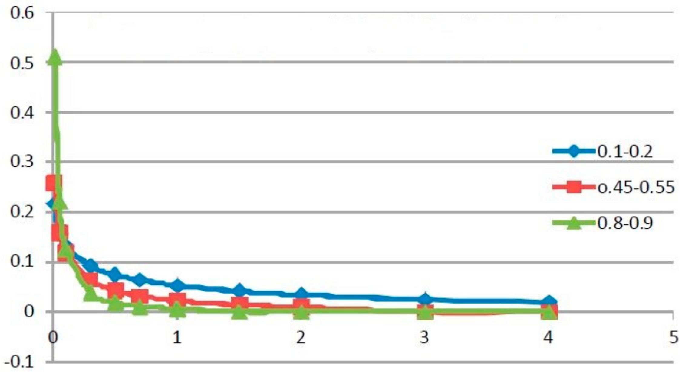
Figure 3.
Comparison of the values of the kernels of Caputo DOFD and Caputo-Fabrizio DOFD when the order is distributed in the interval of integration (0.1–0.2).
Figure 3.
Comparison of the values of the kernels of Caputo DOFD and Caputo-Fabrizio DOFD when the order is distributed in the interval of integration (0.1–0.2).

Figure 4.
Comparison of the values of the kernels of the Caputo DOFD and the Caputo-Fabrizio DOFD when the order is distributed in the interval of integration 0.45–0.55.
Figure 4.
Comparison of the values of the kernels of the Caputo DOFD and the Caputo-Fabrizio DOFD when the order is distributed in the interval of integration 0.45–0.55.
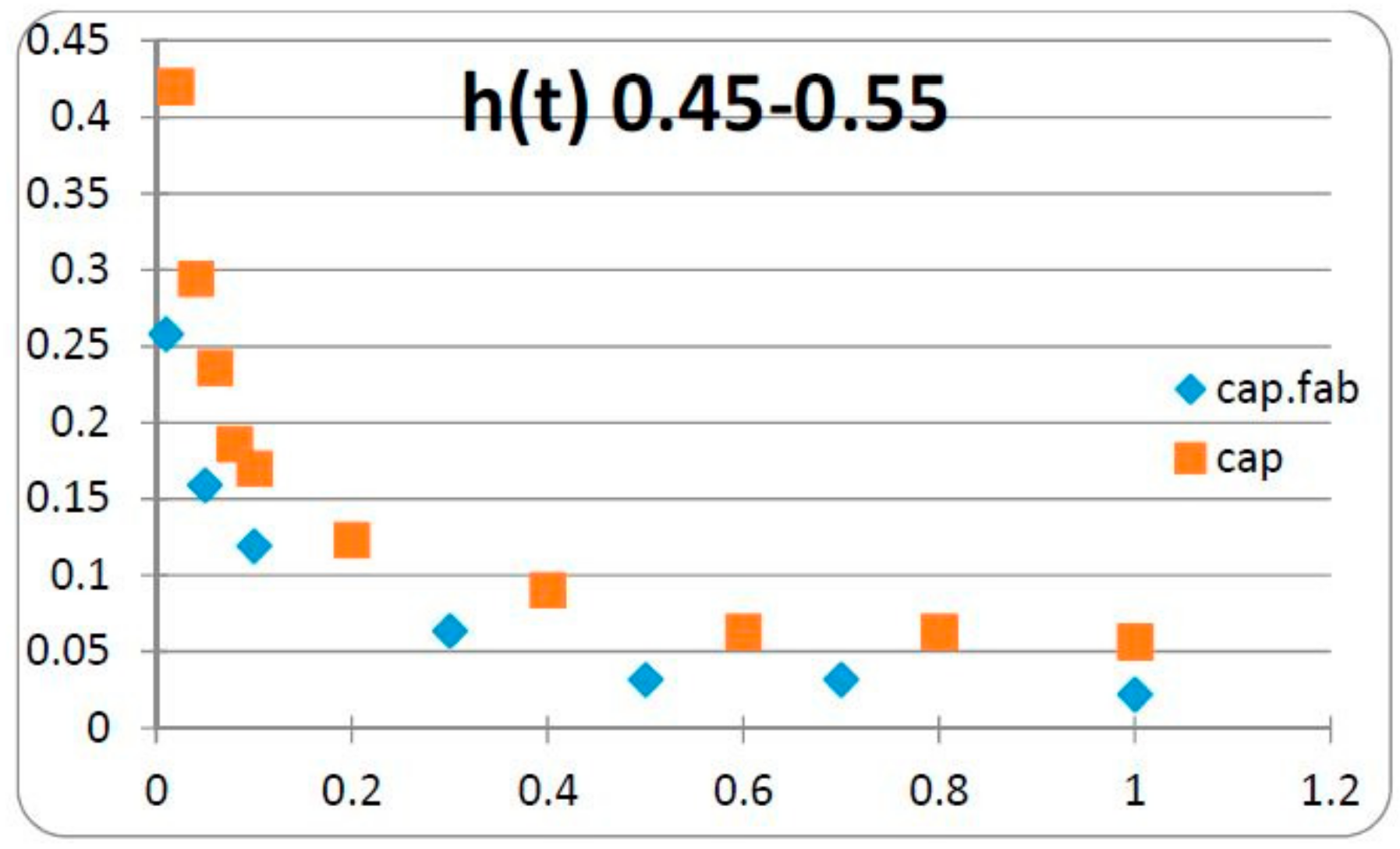
Figure 5.
Comparison of the values of the kernels of the Caputo DOFD and the Caputo-Fabrizio DOFD when the order is distributed in the interval of integration 0.8–0.9.
Figure 5.
Comparison of the values of the kernels of the Caputo DOFD and the Caputo-Fabrizio DOFD when the order is distributed in the interval of integration 0.8–0.9.
© 2017 by the authors. Licensee MDPI, Basel, Switzerland. This article is an open access article distributed under the terms and conditions of the Creative Commons Attribution (CC BY) license (http://creativecommons.org/licenses/by/4.0/).
Share and Cite
MDPI and ACS Style
Caputo, M.; Fabrizio, M. The Kernel of the Distributed Order Fractional Derivatives with an Application to Complex Materials. Fractal Fract. 2017, 1, 13. https://doi.org/10.3390/fractalfract1010013
AMA Style
Caputo M, Fabrizio M. The Kernel of the Distributed Order Fractional Derivatives with an Application to Complex Materials. Fractal and Fractional. 2017; 1(1):13. https://doi.org/10.3390/fractalfract1010013
Chicago/Turabian StyleCaputo, Michele, and Mauro Fabrizio. 2017. "The Kernel of the Distributed Order Fractional Derivatives with an Application to Complex Materials" Fractal and Fractional 1, no. 1: 13. https://doi.org/10.3390/fractalfract1010013