A Solution to the Time-Scale Fractional Puzzle in the Implied Volatility

1
Mizuho Securities Co. Ltd., Tokyo 100-0004, Japan
2
Master of Finance Program, Tokyo Metropolitan University, Tokyo 100-0005, Japan
*
Author to whom correspondence should be addressed.
Fractal Fract. 2017, 1(1), 14; https://doi.org/10.3390/fractalfract1010014
Submission received: 28 October 2017
/
Revised: 22 November 2017
/
Accepted: 22 November 2017
/
Published: 25 November 2017
(This article belongs to the Special Issue Fractional Calculus in Economics and Finance)
Abstract
:In the option pricing literature, it is well known that (i) the decrease in the smile amplitude is much slower than the standard stochastic volatility models and (ii) the term structure of the at-the-money volatility skew is approximated by a power-law function with the exponent close to zero. These stylized facts cannot be captured by standard models, and while (i) has been explained by using a fractional volatility model with Hurst index , (ii) is proven to be satisfied by a rough volatility model with under a risk-neutral measure. This paper provides a solution to this fractional puzzle in the implied volatility. Namely, we construct a two-factor fractional volatility model and develop an approximation formula for European option prices. It is shown through numerical examples that our model can resolve the fractional puzzle, when the correlations between the underlying asset process and the factors of rough volatility and persistence belong to a certain range. More specifically, depending on the three correlation values, the implied volatility surface is classified into four types: (1) the roughness exists, but the persistence does not; (2) the persistence exists, but the roughness does not; (3) both the roughness and the persistence exist; and (4) neither the roughness nor the persistence exist.
1. Introduction
In the finance literature, there has been a general consensus that volatility is highly persistent. There are numerous pieces of evidence that the price dynamics of financial products are consistent with fractional Brownian motion (fBM) volatility models with Hurst index , which implies that the volatility has a long memory. See, e.g., [1] for the existence of the long memory features in stock market volatilities. However, inconsistent with this stylized fact, [2] recently find that the log-volatility behaves essentially as an fBM with H close to zero at any reasonable time scale, by estimating the volatility from high frequency data. This puzzle (the word “puzzle” is used in the context of using a fractional volatility model in option pricing, but not used in the context of finance in general) has not been resolved, although one possible explanation may be the smoothing effect by sampling intervals of data. Recall that if , the fBM is the standard Brownian motion (BM), which is a Markov process with short memory. Hence, the fact implies that volatility is rough.
On the other hand, in the context of option pricing, there are also seemingly two inconsistent stylized facts. Namely, (i) the decrease in the smile amplitude is much slower than the standard stochastic volatility models; and (ii) the term structure of the at-the-money volatility skew is well approximated by a power-law function with the exponent close to zero. It is well recognized that the two phenomena cannot be captured by standard models. Nevertheless, in the option pricing literature, these problems have been studied separately.
The fact (i) seems a result of long memory feature of volatility and is indeed explained in [3,4] by using the fractional volatility model with under a risk-neutral measure . They start with a fractional volatility model with under the physical measure , and assuming that the market price of volatility risk is zero, they transform the model to that under . While [3] showed that, thanks to the long memory feature of volatility with , the model can explain the slow decay of the smile amplitude, [4] developed an approximation formula for option prices and confirm the result numerically when .
The fact (ii) is also well-known from empirical observations and has been paid much attention in the finance literature. While there have been several attempts to explain this stylized fact, (see, e.g., [5,6,7] for possible models that explain this stylized fact), Alòs et al. [6] and Fukasawa [8] proved that a fractional volatility model with H close to zero under can have this stylized fact for small T. In other words, they show that the volatility is rough under the risk-neutral measure for short maturity options.
The aim of this paper is to provide a solution to the time-scale fractional puzzle in the implied volatility. To this end, we adopt the fractional volatility model considered in [4] and extend it by introducing another fractional volatility factor with Hurst index . Following the same idea as in [4], we develop an approximation formula for European option prices and confirm that our model can incorporate both persistence and roughness in the volatility under the risk-neutral measure , when the correlations between the underlying asset process and the factors of rough volatility and persistence belong to a certain range.
An important finding in this paper is that, depending on the three correlation values, the implied volatility surface is classified into four types: (1) the roughness exists, but the persistence does not; (2) the persistence exists, but the roughness does not; (3) both the roughness and the persistence exist; and (4) neither the roughness nor the persistence exist. Hence, the coexistence of the two stylized facts requires the two-factor fractional volatilities of roughness and persistence in a non-trivial manner.
This paper is organized as follows. In the next section, we set up our two-factor fractional volatility model. By using the technique developed in [4], we derive an approximation formula for option prices in Section 3. Section 4 is devoted to numerical examples to investigate the impact of the two Hurst indexes on option prices. Through our extensive numerical experiments, we confirm that our model can resolve the implied volatility puzzle mentioned above. The definitions of the functions contained in our approximation formula are given in Appendix A.
2. The Setup
Inspired by the model proposed in [4], we consider the following two-factor fractional volatility model. Namely, the underlying asset price and its volatility are modeled by the stochastic differential equations (SDEs):
under the physical measure , where is the instantaneous mean rate of return of the asset, q is the (constant) dividend rate and is some smooth function in x and y. Here, while is a standard Brownian motion (BM), denotes a fractional Brownian motion (fBM) with Hurst index under . The volatility is formulated by using the two fractional mean-reverting processes . Note that represents the long-term average of , is the speed of mean reversion and is the volatility of . Later, we specify and , because we want to explain the persistent volatility and rough volatility simultaneously.
2.1. Integral Representation
The fBM can be represented in terms of the stochastic integral with respect to another standard BM. In this study, we find it useful for the development of our approximation to employ the Mandelbrot–Van Ness representation of fBMs. Namely, we have:
where denotes the gamma function and where is a standard BM with constant correlations and , . By defining:
and:
we then have the following representation:
Note that, given , the future behavior of , , is independent of the past, because the BM is a Markov process. Hence, supposing that the past , has been observed, the quantity is considered to be a deterministic function of time with .
By applying the integration-by-parts formula and changing the order of integration, the volatility can be rewritten as:
where:
See [4] for the detailed derivation.
Now, we introduce the market prices of risks and to define the standard BMs and under a martingale measure . Namely, define:
respectively. It follows from (1) and the standard argument that the asset price follows the SDE:
under , where r denotes the risk-free spot rate, which we assume to be constant for simplicity.
By applying Ito’s formula, we obtain:
where is the forward price of the underlying asset with delivery date t. On the other hand, the fractional mean-reverting process is given by:
where:
Summarizing, our fractional volatility model is formulated as:
for , where and , .
2.2. Some Special Cases
Recall that we suppose the past , has been observed and the quantity is a deterministic function of time with . However, it seems difficult to observe the whole past of in the actual market, and so, we assume that as in [3] in the rest of this paper. Furthermore, following most of the previous research, we assume that the volatility risks are fully diversified, and so, the market prices of risks are zero, i.e., , for the sake of simplicity. Under these specifications, the fractional mean-reverting process is given by:
where is defined in (4). Given these processes , the dynamics of the asset price is determined by the SDE (5).
We observe from (8) that the process is a sum of a deterministic function and a stochastic convolution , where:
respectively. For the purpose of Monte Carlo simulation, we consider the discrete-time process , , where is the option maturity for sufficiently small . The stochastic convolution can be approximated by a discrete convolution such as , where and .
The discrete convolution can be represented by a matrix product, and so, the mean-reverting process , , in discrete time can be expressed compactly in matrix form as:
3. Approximation Formula
The call option price written on with strike K and maturity T is given by:
where , and the expectation is taken over under the martingale measure . In this case, all we need to know is the distribution of asset price at the maturity T.
Let us define . From (10), the value of the European call option is given by:
With the density function of at hand, it follows that:
In this section, we derive an approximation formula for option prices by applying the technique used in [4] for the fractional volatility model (7). To this end, we expand the underlying asset into a sum of iterative stochastic integrals with deterministic integrands. In the following, we denote and
The proof of the next result is given in Appendix A.
Lemma 1.
For , we approximate it by:
where:
with:
and with being defined by:
Following the idea given in [10], the density function can be approximated by given in (A16) in Appendix B. By computing (11), the next result then follows. The proof is straightforward, although messy, and omitted.
Proposition 1.
The value of a European call option with maturity T and strike K under the fractional volatility model (7) is approximated as:
where is the density function of the normal distribution with mean μ and variance and denotes the cumulative probability function of the standard normal distribution.
The definitions of , and are provided in Appendix B.
4. Numerical Examples
This section is devoted to numerical studies of our fractional volatility model by using the approximation formula given in Proposition 1. (The accuracy of our approximation formula is checked by the Monte Carlo simulation explained in Section 2.2. We note that our approximation gets gradually worse for the high volatility, long maturity and deep in-the and out-of-the money cases. For example, when the percentage volatility defined by is bigger than , our approximation seems not enough for practical uses. For such cases, higher order approximation is required.) Throughout the numerical examples, we use the parameter values listed in Table 1 as the base case. In particular, for the Hurst indexes and , Bollerslev and Mikkelsen [1] observed long memory features in stock market volatilities, and so, we set as the persistent volatility. On the other hand, Bayer et al. [11] claimed (they report a good fit of their rough volatility model with and the percentage volatility ) that is of order 0.1, and so, we set as the rough volatility. Finally, we assume that the volatility function is given by:
for the sake of simplicity.
In Figure 1, we depict the ATM (at the money) implied volatility (Figure 1a) and the ATM skew (Figure 1b) with respect to the option maturity T. It is observed that the term structure of the ATM volatility skew is a power-law function of time to maturity T. This is a typical feature of rough volatility, which is observed in the S&P index options market reported by Bayer et al. [11]. The model ATM skew is approximated by the power-law function with the order of .
Next, based on our approximation formula, we investigate the effects of the model parameters on option prices.
4.1. Effect of
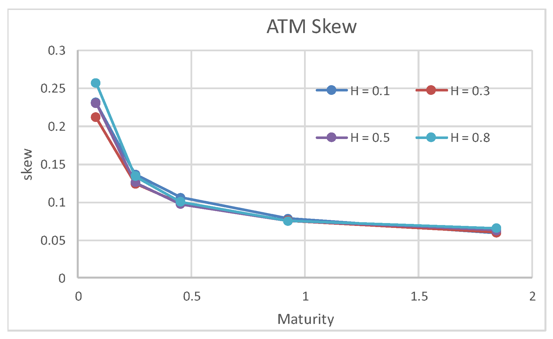
In Figure 2, we plot the skew of the European options with respect to . It is explicitly observed that, as increases, the power-law index increases to be , , and for and , respectively. According to [5], an empirical study shows that the index is typically given by about , and so, our model is capable of capturing this stylized fact by setting the rough volatility close to zero.
4.2. Effect of
We first check whether the Hurst index of persistent volatility has the ability to capture the power-law of the ATM skew or not. Figure 3 shows the ATM skew of the European options with respect to . In contrast to the rough volatility index given in Figure 2, the effect of on the ATM skew is very limited or almost has no effect. On the other hand, Figure 4 shows the volatility smile with respect to the strike and maturity.
Figure 4a–d show the volatility smile of , , and , respectively. From Figure 4, thanks to the long memory feature of the index , the case of exhibits a slower decrease of the volatility smile amplitude with respect to time to maturity T than the short memory case (the rough volatility case shows a much faster decrease). This is a preferable feature, because the observed smile amplitude decreases much more slowly with respect to maturity than that explained by standard stochastic volatility models.
Summarizing, an important observation at this point is that, by setting and , we can realize both the long memory feature and the roughness of volatility simultaneously by using our model, which is the major contribution of this paper.
4.3. Effect of and
We examine the impact of on option prices. Recall that is the correlation between the persistent volatility and the rough volatility . Note that the ATM skew amplitude comes from the roughness of .
From Figure 5, it is observed that, as the correlation decreases, the decrease of the smile amplitude is decelerated in the case of . This means that the effect of the volatility persistence survives only when the correlation is negative.
4.4. Effect of Correlations
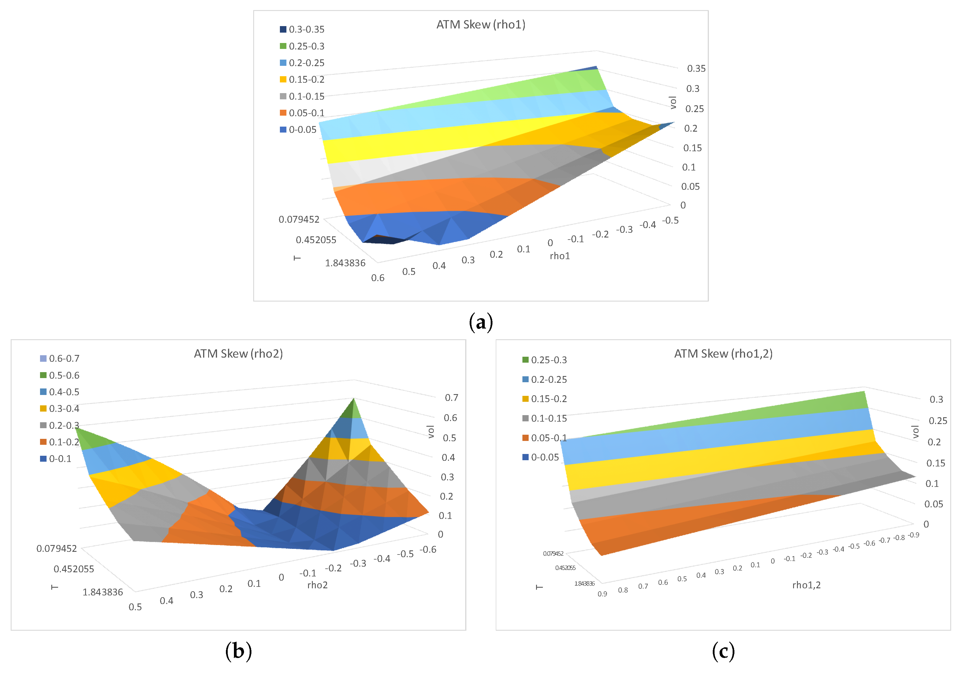
Finally, we examine the effect of the correlations, (, , ), on the implied volatility surface. Figure 6a–c and Figure 7a–c, respectively) show the volatility smile (the ATM skew) at with respect to , and , respectively. The three correlations vary in the range of , and , where the resulting correlation matrix is positive definite. The other parameters are set to be the same as the base case in Table 1.
As we can see form the figures, depending on the correlation values, the volatility surface is classified into four types: (1) the roughness exists, but the persistence does not; (2) the persistence exists, but the roughness does not; (3) both the roughness and the persistence exist; and (4) neither the roughness nor the persistence exist.
Specifically, as increases, it is observed from Figure 6a and Figure 7a that the volatility smile is preserved and the skew becomes greater, i.e., the power-law index of the ATM skew decreases, respectively. Form Figure 6b and Figure 7b, when the absolute value of is small, say , it is observed that the volatility smile is preserved, but the ATM skew disappears, respectively. On the other hand, when the absolute value of is high, say , we can see that the volatility smile gradually disappears, but the ATM skew becomes greater. Furthermore, from Figure 6c and Figure 7c, as increases, the ATM skew becomes greater, but the volatility smile disappears, respectively.
5. Conclusions
In this study, we extend the fractional volatility model proposed in [4] by introducing another factor of rough volatility. Through numerical experiments, we demonstrate that, when one of the Hurst indexes in fractional volatility is larger than 1/2 (volatility persistence) and the other is smaller than 1/2 (rough volatility), our model can explain both the slower decay of the smile amplitude decline and the term structure of the at-the-money volatility skew observed in the options market, simultaneously. However, the coexistence of the two stylized facts seems non-trivial. Namely, depending on the three correlation values between the underlying asset and the factors of rough volatility and volatility persistence, the implied volatility surface is classified into four types: (1) the roughness exists, but the persistence does not; (2) the persistence exists, but the roughness does not; (3) both the roughness and the persistence exist; and (4) neither the roughness nor the persistence exist.
As future work, we plan to apply our model to actual markets. Namely, we develop a fast algorithm to calibrate our model to the options market, because our model involves many parameters itself. Furthermore, it is of interest to develop a model under the physical measure to explain the volatility persistence and the volatility roughness simultaneously. An asymmetric model between the persistent volatility and the rough volatility may be of great importance.
Acknowledgments
Masaaki Kijima is grateful for the research grants funded by the Grant-in-Aid (A) (#26242028) from Japan’s Ministry of Education, Culture, Sports, Science and Technology.
Author Contributions
Hideharu Funahashi and Masaaki Kijima wrote the paper. Hideharu Funahashi conceived and performed the experiments, and Hideharu Funahashi and Masaaki Kijima analyzed the data.
Conflicts of Interest
The authors declare no conflict of interest.
Appendix A. Proof of Lemma 1
For the proof of Lemma 1, we apply the chaos expansion approach proposed by [12]. Namely, consider the solution (6), i.e.,
Denoting and , by means of the Hermite expansion, we have:
where denotes the Hermite polynomial of order n. See [12] for details.
Let , and define:
It then follows that:
where:
Our approximation is to truncate the infinite sum at . As we shall show later, this approximation corresponds to neglecting a sum of iterated integrals:
at . If the volatilities are deterministic functions and is sufficiently small, then Proposition 2.2 of [12] assures that the sum of the iterated integrals converges very quickly.
Before proceeding, since is the deterministic function of s, we can apply the Wiener–Ito chaos expansion to to obtain
Hence, we define:
as an approximation for .
Summarizing, we approximate the quantity by:
where is given by (A4) and by (A3). In the following, we approximate each by an iterated integral with deterministic volatilities.
In this paper, we employ Taylor’s expansion around for this purpose. Recall that . It follows that:
and
where we denote:
for the sake of notational simplicity.
We next approximate each by using the approximations (A6) and (A7). Since , from (A6) and (7), we get:
Moreover, by applying Ito’s formula, the second term on the left-hand side of (A8) is written as:
Hence, we have:
From the definition, we have:
However, from (A7) and (7), we obtain:
Note that, by Ito’s formula, the second and fourth terms in (A11) are written by:
and:
respectively. Hence, inserting (A12) and (A13) into (A11), we get:
Finally, inserting (A4), (A10) and (A14) into (A5), we obtain the desired result.
Appendix B. Derivation of the Approximated Density Function
In this Appendix, we obtain an approximation formula for the density function of . To this end, note that (7) is a special case of Equation (2) in [10]. Hence, applying Proposition 3.2 in [10], the following result can be obtained.
First, note that in Lemma 1 follows a normal distribution with zero mean and variance . Then, by applying the following result, an approximation of the density function of can be obtained. The proof is found in [12] under a general setting.
Lemma A1.
Let us denote the density function of by . Then, the probability density function of is approximated as:
where denotes the normal density function with mean a and variance b.
The conditional expectations in Lemma A1 can be evaluated explicitly by using the formulas provided in Appendix C. Namely, we obtain:
where:
, , and . Here, we define:
and
By substituting the conditional expectations into (A15), the approximate density function, denoted by , can be expressed as:
where denotes the Hermite polynomial of order n:
with .
Appendix C. Formulas for Conditional Expectations
Let , , be the standard Brownian motions with correlation , and let , , be deterministic functions of time. Moreover, let , and denote . Then, the following formulas are well known: First,
where:
Next,
where:
Finally,
where:
References
- Bollerslev, T.; Mikkelsen, H.O. Modeling and Pricing Long Memory in Stock Market Volatility. J. Econom. 1996, 73, 151–184. [Google Scholar] [CrossRef]
- Gatheral, J.; Jaisson, T.; Rosenbaum, M. Volatility is rough. arXiv, 2014; arXiv:1410.3394. [Google Scholar]
- Comte, F.; Renault, E. Long memory in continuous-time stochastic volatility models. Math. Financ. 1998, 8, 291–323. [Google Scholar] [CrossRef]
- Funahashi, H.; Kijima, M. Does the Hurst index matter for option prices under fractional volatility? Ann. Financ. 2017, 17, 189–198. [Google Scholar] [CrossRef]
- Fouque, J.P.; Papanicolaou, G.; Sircar, R.; Solna, K. Maturity cycles in implied volatility. Financ. Stoch. 2004, 8, 451–477. [Google Scholar] [CrossRef]
- Alòs, E.; León, J.A.; Vives, J. On the short-time behavior of the implied volatility for jump-diffusion models with stochastic volatility. Financ. Stoch. 2007, 11, 571–589. [Google Scholar] [CrossRef]
- Fukasawa, M. Short-time at-the-money skew and rough fractional volatility. Quant. Financ. 2017, 17, 189–198. [Google Scholar] [CrossRef]
- Fukasawa, M. Asymptotic analysis for stochastic volatility: Martingale expansion. Financ. Stoch. 2011, 15, 635–654. [Google Scholar] [CrossRef]
- Kijima, M.; Tam, C.M. Fractional Brownian motions in financial models and their Monte Carlo simulation. In Theory and Applications of Monte Carlo Simulations; Chan, W.K., Ed.; InTech: Rijeka, Croatia, 2013; pp. 53–85. [Google Scholar]
- Funahashi, H. A chaos expansion approach under hybrid volatility models. Quant. Financ. 2014, 14, 1923–1936. [Google Scholar] [CrossRef]
- Bayer, C.; Friz, P.; Gatheral, J. Pricing under rough volatility. Quant. Financ. 2016, 16, 887–904. [Google Scholar] [CrossRef]
- Funahashi, H.; Kijima, M. A chaos expansion approach for the pricing of contingent claims. J. Comput. Financ. 2015, 18, 27–58. [Google Scholar] [CrossRef]
Figure 1.
ATM implied volatility (a) and ATM skew (b) with respect to the option maturity. The model parameters are listed in Table 1.
Figure 1.
ATM implied volatility (a) and ATM skew (b) with respect to the option maturity. The model parameters are listed in Table 1.

Figure 2.
ATM skew with respect to , where denotes the Hurst index of the rough volatility. The model parameters are listed in Table 1.
Figure 2.
ATM skew with respect to , where denotes the Hurst index of the rough volatility. The model parameters are listed in Table 1.
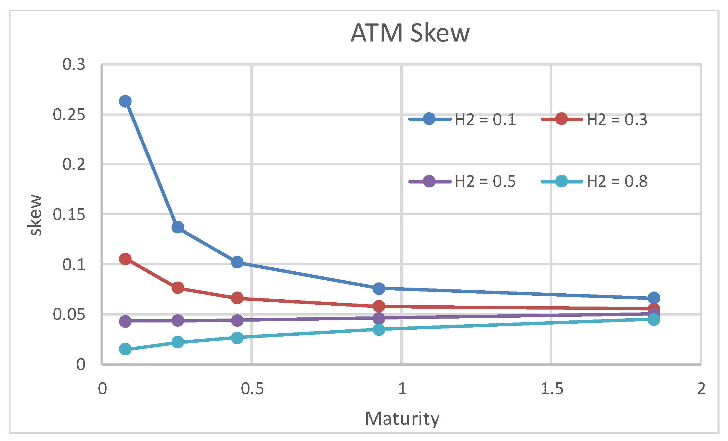
Figure 3.
ATM skew with respect to , the Hurst index of volatility persistence. The model parameters are listed in Table 1.
Figure 3.
ATM skew with respect to , the Hurst index of volatility persistence. The model parameters are listed in Table 1.

Figure 4.
Volatility smile with respect to strike and maturity. (a–d) show the volatility smile of , , , and , respectively. The model parameters are listed in Table 1.
Figure 4.
Volatility smile with respect to strike and maturity. (a–d) show the volatility smile of , , , and , respectively. The model parameters are listed in Table 1.
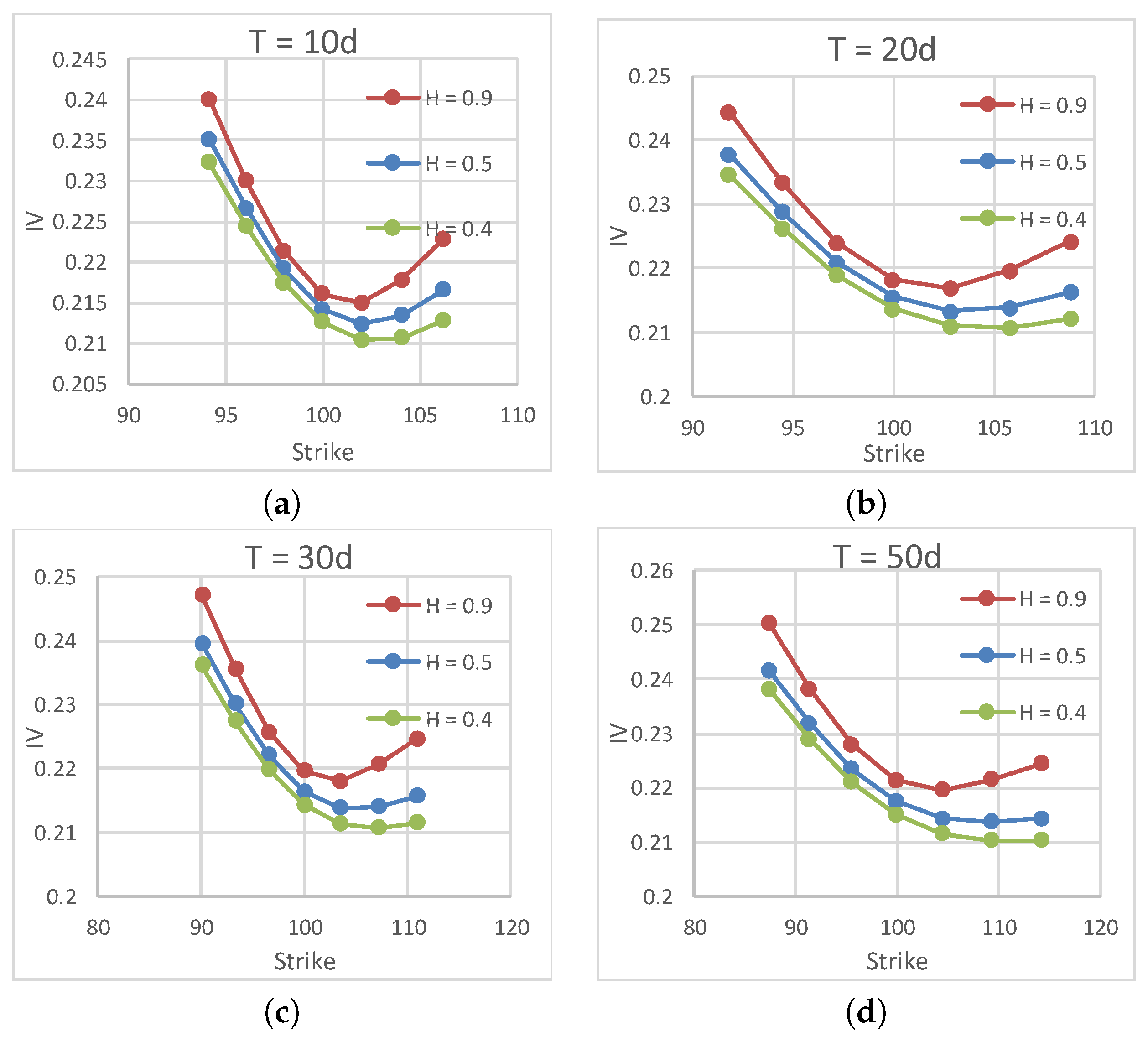
Figure 5.
Volatility smile with respect to correlation . (a–c) show the volatility smile of , 0, and , respectively. The maturity is and the other parameters are listed in Table 1.
Figure 5.
Volatility smile with respect to correlation . (a–c) show the volatility smile of , 0, and , respectively. The maturity is and the other parameters are listed in Table 1.
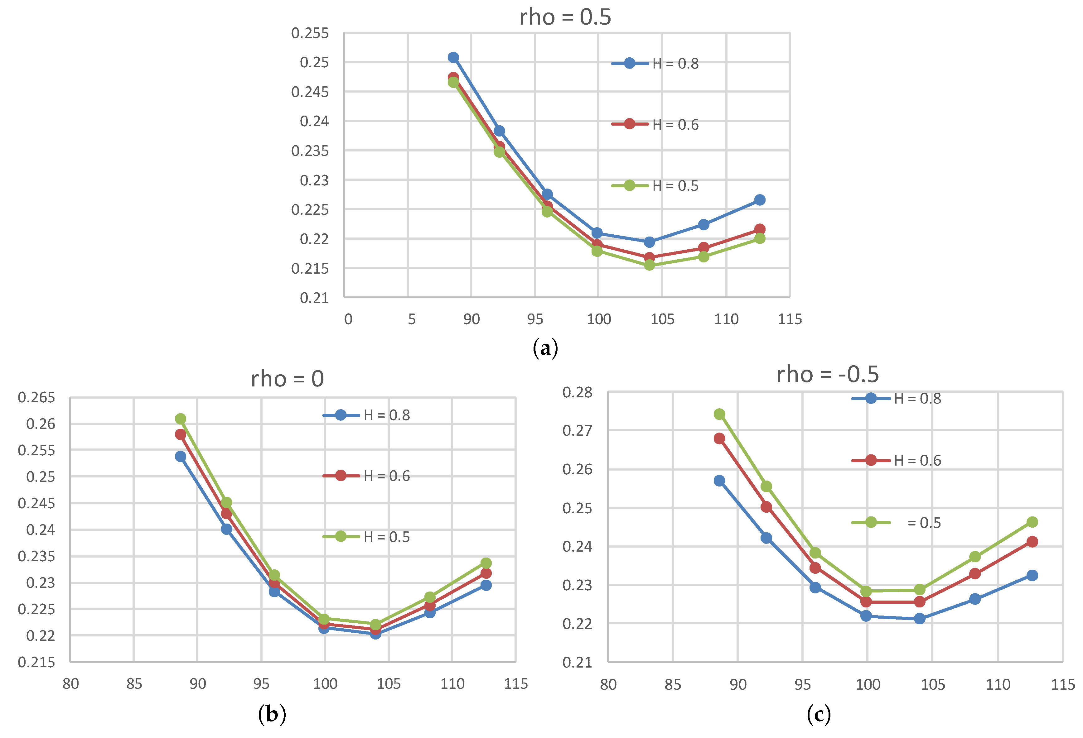
Figure 6.
Volatility smile with respect to the correlations. (a–c) show the volatility smile of , , and , respectively. The maturity is and the other parameters are listed in Table 1.
Figure 6.
Volatility smile with respect to the correlations. (a–c) show the volatility smile of , , and , respectively. The maturity is and the other parameters are listed in Table 1.
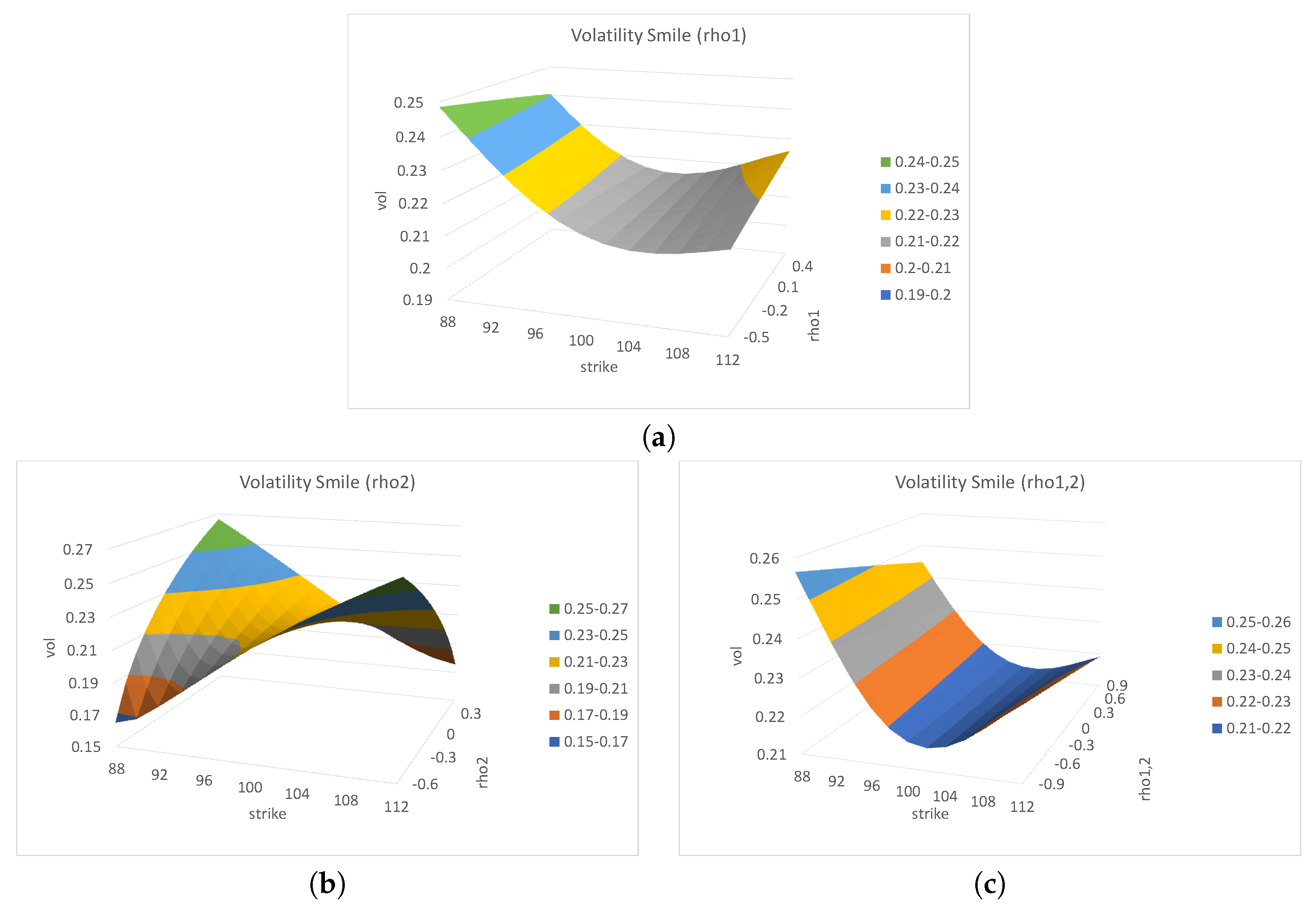
Figure 7.
ATM skew with respect to the correlations. (a–c) show the ATM skew of , , and , respectively. The other parameters are listed in Table 1.
Figure 7.
ATM skew with respect to the correlations. (a–c) show the ATM skew of , , and , respectively. The other parameters are listed in Table 1.

Table 1.
Base case parameters.
| r | q | |||||||||||||
|---|---|---|---|---|---|---|---|---|---|---|---|---|---|---|
| 100 | 0.0131 | 0.017 | 0.2 | 0.0 | 0.0 | 0.0 | 0.0 | 0.0 | 0.12 | 0.12 | 0.8 | 0.1 |
© 2017 by the authors. Licensee MDPI, Basel, Switzerland. This article is an open access article distributed under the terms and conditions of the Creative Commons Attribution (CC BY) license (http://creativecommons.org/licenses/by/4.0/).
Share and Cite
MDPI and ACS Style
Funahashi, H.; Kijima, M. A Solution to the Time-Scale Fractional Puzzle in the Implied Volatility. Fractal Fract. 2017, 1, 14. https://doi.org/10.3390/fractalfract1010014
AMA Style
Funahashi H, Kijima M. A Solution to the Time-Scale Fractional Puzzle in the Implied Volatility. Fractal and Fractional. 2017; 1(1):14. https://doi.org/10.3390/fractalfract1010014
Chicago/Turabian StyleFunahashi, Hideharu, and Masaaki Kijima. 2017. "A Solution to the Time-Scale Fractional Puzzle in the Implied Volatility" Fractal and Fractional 1, no. 1: 14. https://doi.org/10.3390/fractalfract1010014