Series Solution of the Pantograph Equation and Its Properties

1
Department of Mathematics, Shivaji University, Kolhapur 416004, India
2
Ashokrao Mane Group of Institution, Vathar, Kolhapur 416112, India
*
Author to whom correspondence should be addressed.
Fractal Fract. 2017, 1(1), 16; https://doi.org/10.3390/fractalfract1010016
Submission received: 26 October 2017
/
Revised: 28 November 2017
/
Accepted: 30 November 2017
/
Published: 8 December 2017
(This article belongs to the Special Issue The Craft of Fractional Modelling in Science and Engineering)
Abstract
:In this paper, we discuss the classical pantograph equation and its generalizations to include fractional order and the higher order case. The special functions are obtained from the series solution of these equations. We study different properties of these special functions and establish the relation with other functions. Further, we discuss some contiguous relations for these special functions.
Keywords:
pantograph equation; proportional delay; fractional derivative; Gaussian binomial coefficientMSC:
33E99; 34K06; 34K071. Introduction
Ordinary differential equations (ODE) are widely used by researchers to model various natural systems. However, it is observed that such equations cannot model the actual behavior of the system. Since the ordinary derivative is a local operator, it cannot model the memory and hereditary properties in real-life phenomena. Such phenomena can be modeled in a more accurate way by introducing some nonlocal component, e.g., delay in it.
The characteristic equation of delay differential equations (DDE) is a transcendental equation in contrast with the polynomial in the case of ODE. Hence, the DDEs are difficult to analyze as compared with ODEs.
Various special functions viz. exponential, sine, cosine, hypergeometric, Mittag-Leffler and gamma are obtained from ODEs [1]. If the equations have variable coefficients, then we may get the Legendre polynomial, the Laguerre polynomial, Bessel functions, and so on [2]. However, there are vary few papers that are devoted to the special functions arising in DDEs [3]. This motivates us to work on the special functions emerging from the solution of DDE with proportional delay. We analyze different properties of such special functions and present the relationship with other functions.
2. Preliminaries
Definition 1
Definition 2
Definition 3
Definition 4
([6]). Two special functions are said to be contiguous if their parameters differ by integers. The relations made by contiguous functions are said to be contiguous function relations.
Theorem 1
([7]). (Existence and uniqueness theorem)
Let X be a Banach space and . If is continuous and there exists a positive constant , such that , , and if , then the fractional differential equation with proportional delay:
where , has a unique solution.
3. Pantograph Equation
The pantograph is a current collection device, which is used in electric trains. The mathematical model of the pantograph is discussed by various researchers [8,9,10,11].
The differential equation:
with proportional delay modeling these phenomena is discussed by Ockendon and Tayler in [12]. Equation (4) is called the pantograph equation. Kato and McLeod [13] showed that the problem (4) is well-posed if . Further, the authors discussed the asymptotic properties of this equation. The coefficients in the power series solution are obtained by using a recurrence relation.
Iserles [15] considered a generalized pantograph equation where . The condition for the well-posedness of the problem is given in terms of and C. The solution of the problem is expressed in the form of the Dirichlet series. Further, the advanced pantograph equation , where and for all , is also analyzed by Derfel and Iserles [16]. In [17], Patade and Bhalekar discussed the pantograph equation with incommensurate delay. Various properties of the series solution obtained are discussed.
4. Special Function Generated from the Pantograph Equation
We write solution (5) in the form of following special function:
The notation is used in memory of Ramanujan [18].
Theorem 2
Corollary 1.
The power series (6) is absolutely convergent for all t, and hence, it is uniformly convergent on any compact interval on .
Theorem 3.
For , we have:
Proof.
Consider:
Hence the proof. ☐
Theorem 4.
For , we have:
Proof.
We prove the result by using the induction hypothesis on m.
From Theorem 3, the result is true for .
Suppose,
Consider,
Using Theorem 3, we have:
This completes the proof. ☐
Theorem 5.
For , we have:
Theorem 6.
If , then we can express the integral of in the following series containing binomial coefficients:
Proof.
Consider:
☐
Theorem 7.
If , then we have the following relation:
Proof.
Consider:
☐
Theorem 8.
The function shows the following relationship with the lower incomplete gamma function γ:
Proof.
We have:
By using the property [20]: , we get
☐
Theorem 9.
The following integral gives the relation between the function and the upper incomplete gamma function :
Proof.
By using the property [20]: , we obtain
☐
5. Properties, Relations and Identities of
We state the following properties of without proof.
5.1. Properties of
For :
- .
- (a)
- .
- (b)
- .
- .
- (a)
- .
- (b)
- .
- (c)
- .
- (d)
- .
- (e)
- .
- (f)
- .
- .
- (a)
- .
- (b)
- .
- (c)
- .
- (d)
- .
5.2. Relation to Other Functions
- .
- .
- ,
where and are the incomplete beta function and regularized incomplete beta function [4].
5.3. Contiguous Relations of
- .
- .
- .
6. Generalizations
6.1. Generalizations to Include the Fractional Order Derivative
Consider the fractional delay differential equation with proportional delay:
where , , and .
The solution of (8) is:
We denote the series in (9) by:
Theorem 10.
If , then the power series:
is convergent for all finite values of t.
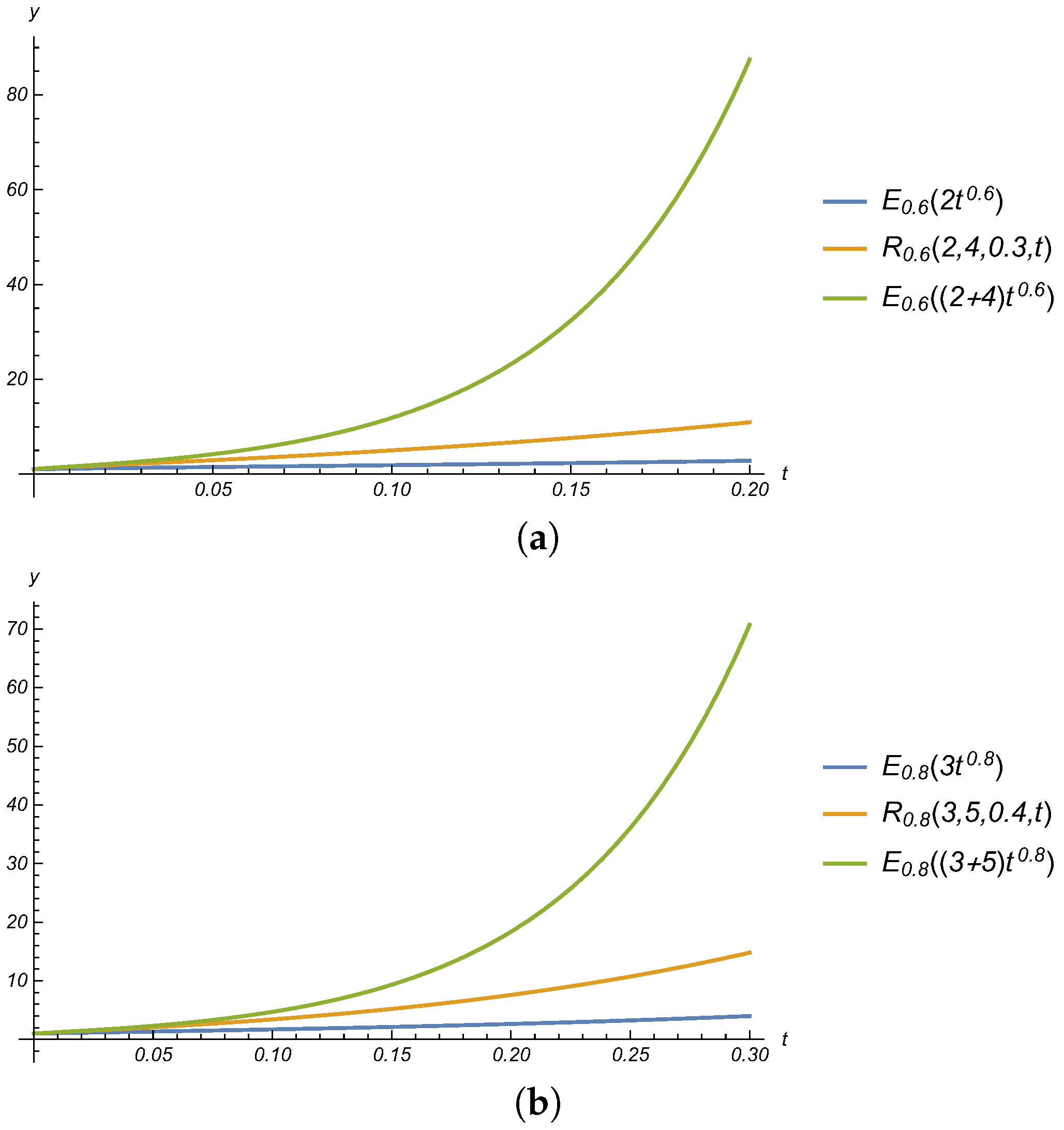
Theorem 11.
For , and , the function satisfies the following inequality:
Proof.
Since , and , we have:
Taking summation over n, we get:
Similarly, we have:
The result is illustrated in Figure 1a,b.
Theorem 12.
For , we have:
Theorem 13.
(Addition theorem)
where
Proof.
We have:
☐
Properties and Relations of
We get the following analogous properties and relations as in Section 5, e.g.,
- .
- .
- and so on.
6.2. Generalizations to the Higher Order Case
Consider the system of delay differential equation with proportional delay:
where , , and
The solution of (12) is:
Theorem 14.
If is invertible for each n, then the power series:
where and is convergent for .
6.3. Properties and Relations of
We get the following analogous properties and relations as in Section 5 under the condition that A, B, and are invertible.
6.3.1. Properties of
- .
- , etc.
6.3.2. Contiguous Relations of
- .
- .
- .
7. Conclusions
In this article, we discussed the pantograph equation and its generalizations. The series solutions of these equations are treated as special functions. These special functions are different from hyper-geometric and other special functions because they are obtained as a solution of the delay differential equation. It is observed that the m-th derivative of can be represented as a linear combination of for with Gaussian binomial coefficients. The function is shown to be bounded by the Mittag-Leffler functions. We have studied different properties and discussed some relations of these special functions. We hope that our work will encourage researchers to dig for more properties of the special functions obtained from delay differential equations.
Acknowledgments
Sachin Bhalekar acknowledges Council of Scientific and Industrial Research (CSIR), New Delhi, for funding through Research Project No. 25(0245)/15/EMR-II.
Author Contributions
Sachin Bhalekar suggested the problem, guided for the research work and confirmed the results. Jayvant Patade obtained the solution to the problem and derived the relations.
Conflicts of Interest
The authors declare no conflict of interest.
References
- Mathai, A.M.; Haubold, H.J. Special Functions for Applied Scientists; Springer: New York, NY, USA, 2008. [Google Scholar]
- Bell, W.W. Special Functions for Scientists and Engineers; Courier Corporation: London, UK, 2004. [Google Scholar]
- Corless, R.M.; Gonnet, G.H.; Hare, D.E.G.; Jeffrey, D.J.; Knuth, D.E. On the Lambert W function. Adv. Comput. Math. 1996, 5, 329–359. [Google Scholar] [CrossRef]
- Magnus, W.; Oberhettinger, F.; Soni, R.P. Formulas and Theorems for the Special Functions of Mathematical Physics; Springer: New York, NY, USA, 2013; Volume 52. [Google Scholar]
- Kilbas, A.A.; Srivastava, H.M.; Trujillo, J.J. Theory and Applications of Fractional Differential Equations; Elsevier: Amsterdam, The Netherlands, 2006. [Google Scholar]
- Erdelyi, A.; Magnus, W.; Oberhettinger, F.; Tricomi, F.G. Higher Transcendental Functions; McGraw–Hill: New York, NY, USA, 1955. [Google Scholar]
- Balachandran, K.; Kiruthika, S.; Trujillo, J.J. Existence of solutions of nonlinear fractional pantograph equations. Acta Math. Sci. 2013, 33, 712–720. [Google Scholar] [CrossRef]
- Andrews, H.I. Third paper: Calculating the behaviour of an overhead catenary system for railway electrification. Proc. Inst. Mech. Eng. 1964, 179, 809–846. [Google Scholar] [CrossRef]
- Abbott, M.R. Numerical method for calculating the dynamic behaviour of a trolley wire overhead contact system for electric railways. Comput. J. 1970, 13, 363–368. [Google Scholar] [CrossRef]
- Gilbert, G.; Davtcs, H.E.H. Pantograph motion on a nearly uniform railway overhead line. Proc. Inst. Electr. Eng. 1966, 113, 485–492. [Google Scholar] [CrossRef]
- Caine, P.M.; Scott, P.R. Single-wire railway overhead system. Proc. Inst. Electr. Eng. 1969, 116, 1217–1221. [Google Scholar] [CrossRef]
- Ockendon, J.; Tayler, A.B. The dynamics of a current collection system for an electric locomotive. Proc. R. Soc. Lond. A Math. Phys. Eng. Sci. 1971, 322, 447–468. [Google Scholar] [CrossRef]
- Kato, T.; McLeod, J.B. The functional-differential equation y′(x) = λy(qx) + by(x). Bull. Am. Math. Soc. 1971, 77, 891–937. [Google Scholar]
- Fox, L.; Mayers, D.; Ockendon, J.R.; Tayler, A.B. On a functional differential equation. IMA J. Appl. Math. 1971, 8, 271–307. [Google Scholar] [CrossRef]
- Iserles, A. On the generalized pantograph functional-differential equation. Eur. J. Appl. Math. 1993, 4, 1–38. [Google Scholar] [CrossRef]
- Derfel, G.; Iserles, A. The pantograph equation in the complex plane. J. Math. Anal. Appl. 1997, 213, 117–132. [Google Scholar] [CrossRef]
- Patade, J.; Bhalekar, S. Analytical Solution of Pantograph Equation with Incommensurate Delay. Phys. Sci. Rev. 2017, 2. [Google Scholar] [CrossRef]
- Kanigel, R. The Man Who Knew Infinity; Washington Square Press: New York, NY, USA, 2015. [Google Scholar]
- Stanley, R.P. Enumerative Combinatorics; Cambridge University Press: Cambridge, UK, 1997. [Google Scholar]
- Gautschi, W.; Harris, F.E.; Temme, N.M. Expansions of the exponential integral in incomplete gamma functions. Appl. Math. Lett. 2003, 16, 1095–1099. [Google Scholar] [CrossRef]
Figure 1.
Bounds on : (a) and ; (b) and .

© 2017 by the authors. Licensee MDPI, Basel, Switzerland. This article is an open access article distributed under the terms and conditions of the Creative Commons Attribution (CC BY) license (http://creativecommons.org/licenses/by/4.0/).
Share and Cite
MDPI and ACS Style
Bhalekar, S.; Patade, J. Series Solution of the Pantograph Equation and Its Properties. Fractal Fract. 2017, 1, 16. https://doi.org/10.3390/fractalfract1010016
AMA Style
Bhalekar S, Patade J. Series Solution of the Pantograph Equation and Its Properties. Fractal and Fractional. 2017; 1(1):16. https://doi.org/10.3390/fractalfract1010016
Chicago/Turabian StyleBhalekar, Sachin, and Jayvant Patade. 2017. "Series Solution of the Pantograph Equation and Its Properties" Fractal and Fractional 1, no. 1: 16. https://doi.org/10.3390/fractalfract1010016