A Fractional Complex Permittivity Model of Media with Dielectric Relaxation


1
Department of Biomedical and Dental Sciences and Morphofunctional Imaging, University of Messina, Via Consolare Valeria c/o A.O.U. Policlinico “G.Martino”, I, 98125 Messina, Italy
2
Engineering Office, Via Matteotti, 89044 Locri, Italy
*
Author to whom correspondence should be addressed.
Fractal Fract. 2017, 1(1), 4; https://doi.org/10.3390/fractalfract1010004
Submission received: 11 August 2017
/
Revised: 25 August 2017
/
Accepted: 25 August 2017
/
Published: 29 August 2017
(This article belongs to the Special Issue Fractional Dynamics)
Abstract
:In this work, we propose a fractional complex permittivity model of dielectric media with memory. Debye’s generalized equation, expressed in terms of the phenomenological coefficients, is replaced with the corresponding differential equation by applying Caputo’s fractional derivative. We observe how fractional order depends on the frequency band of excitation energy in accordance with the 2nd Principle of Thermodynamics. The model obtained is validated with respect to the measurements made on the biological tissues and in particular on the human aorta.
1. Introduction
The frequency domain response function of a media dielectric, well-known how complex permittivity, , one obtains from spectral measurement of electrical displacement field respect to applied electric field :
with , , and f being frequency.
The polarization does not follow instantaneous changes of the applied electric field, so the dielectric material is in a state of non-equilibrium. Dielectric relaxation is a process through which dielectric media reach the state of equilibrium, with one or more time constants in relation to corresponding polarization phenomena. In biological tissues, there are five independent polarization mechanisms corresponding to five dispersion spectrum [1]. Debye [2] has proposed the following complex permittivity to take into account dielectric relaxation corresponding to a linear differential equation of the first order, with constant time :
where is the initial permittivity (high frequency), and is the static permittivity. Several complex permittivity models have been proposed, which approximate the experimental values sufficiently with respect to a given frequency band and for particular dielectrics. In the following order, the Cole–Cole model [3,4], the Cole–Davidson model [5], and the Havriliak–Negami model [6] are presented:
with
with
With reference to the measures of complex permittivity, carried out in [7,8,9,10] on the biological tissues, the Cole–Cole model has been proposed to four dispersion spectrum from 10 to 20 GHz:
where is electric permittivity of free space, are time constants and is conductivity in direct current. In these models (3)–(6), the fractional nature of complex permittivity, due to the presence of the parameter how power the time’s constant , is evident. From the thermodynamic point of view, the dielectric relaxation phenomenon has been extensively treated [11,12,13,14]. In these works, the use of internal variables called phenomenological coefficients led to Debye’s generalized equation with two constants of time:
where , , , , , are algebraic functions of the phenomenological coefficients. Putting in (7), one obtains Debye’s equation. The purpose of this paper is to apply fractional calculus to the phenomenological Equation (7) by obtaining a model of complex permittivity in accordance with experimental values. There are different definitions of fractional derivatives whose application depends on the physical meaning that they represent [15,16,17,18,19,20]. In [21], Caputo and Fabrizio proposed a direct model of complex permittivity that generalizes the above-mentioned models (3)–(6), using Caputo’s fractional derivative. In the fractional model proposed here, it is shown that the possible values of the fractional order must be in agreement with those that can assume the phenomenological coefficients in accordance with the 2nd principle of thermodynamics. Compared to [21], the fractional model here obtained derives from Debye’s generalized Equation (7). In Section 2, Caputo’s fractional derivative is applied to Debye’s generalized phenomenological equation. In Section 3, by applying the fractional transformation of Laplace, the fractional model of complex permittivity is obtained. In Section 4, it is shown that the solution obtained by solving a system of four nonlinear equations, whose unknowns are the phenomenological coefficients, conforms with the 2nd principle of thermodynamics, and the fractional model proposed here is valid in accordance with the experimental results.
2. Fractional Generalized Debye’s Equation
In [11,14], dielectric and magnetic relaxation phenomena are discussed with the aid of the general theory of non-equilibrium thermodynamics. It was shown that a vectorial internal variable, which influences the polarization, gives rise to dielectric relaxation phenomena. If one makes linear this theory and if one neglects cross effects due to electric conduction, heat conduction and viscosity on electric relaxation, the following relaxation equation may be derived:
where
where , , , are the phenomenological coefficients and , are scalar constants.
By applying Caputo’s fractional derivative, one obtains:
Caputo’s fractional derivative of order (here has a signified different from than indicated in Equations (3)–(6)) is:
where is
with for . Equation (23) is the fractional equation corresponding to Debye’s generalized equation (14). Caputo’s fractional derivative coincides, at less than one multiplicative factor , with the convolution operator:
This property is utilized to determine the Laplace’s transform of the fractional derivative:
where
and, assuming ,
with and . If , then is coincident with the Fourier’s transform .
It can be demonstrated similarly that
will be placed at 1 subsequently.
3. The Fractional Model
For , one obtains a Ciancio–Kluitenberg model of the complex permittivity:
with = [rad/s], = [rad/s], = [rad/s], = [rad/s].
4. Numerical Results
The fractional model of the complex permittivity (36) is determined uniquely from the possible values of the parameters , , , that satisfaction (36) with , ; this is in accordance with the fact that entropy variation is positive, reference [11], for the 2nd principle of the thermodynamics. The fractional order depends on the frequency and parameters by means of undefined function. In [3], the Debye’s ordinary model is in accordance with experimental measures at low frequencies. We can formulate the problem in this way:
Let , and let be the solutions set of the system nonlinear equations:
with unknown and , , , , known experimental, while is value of such that solution of system (45) indicated with satisfaction (36), and it provides the best predictive model of complex permittivity.
In other words, if , where is unknown function of , denoting with , we have that is:
with .
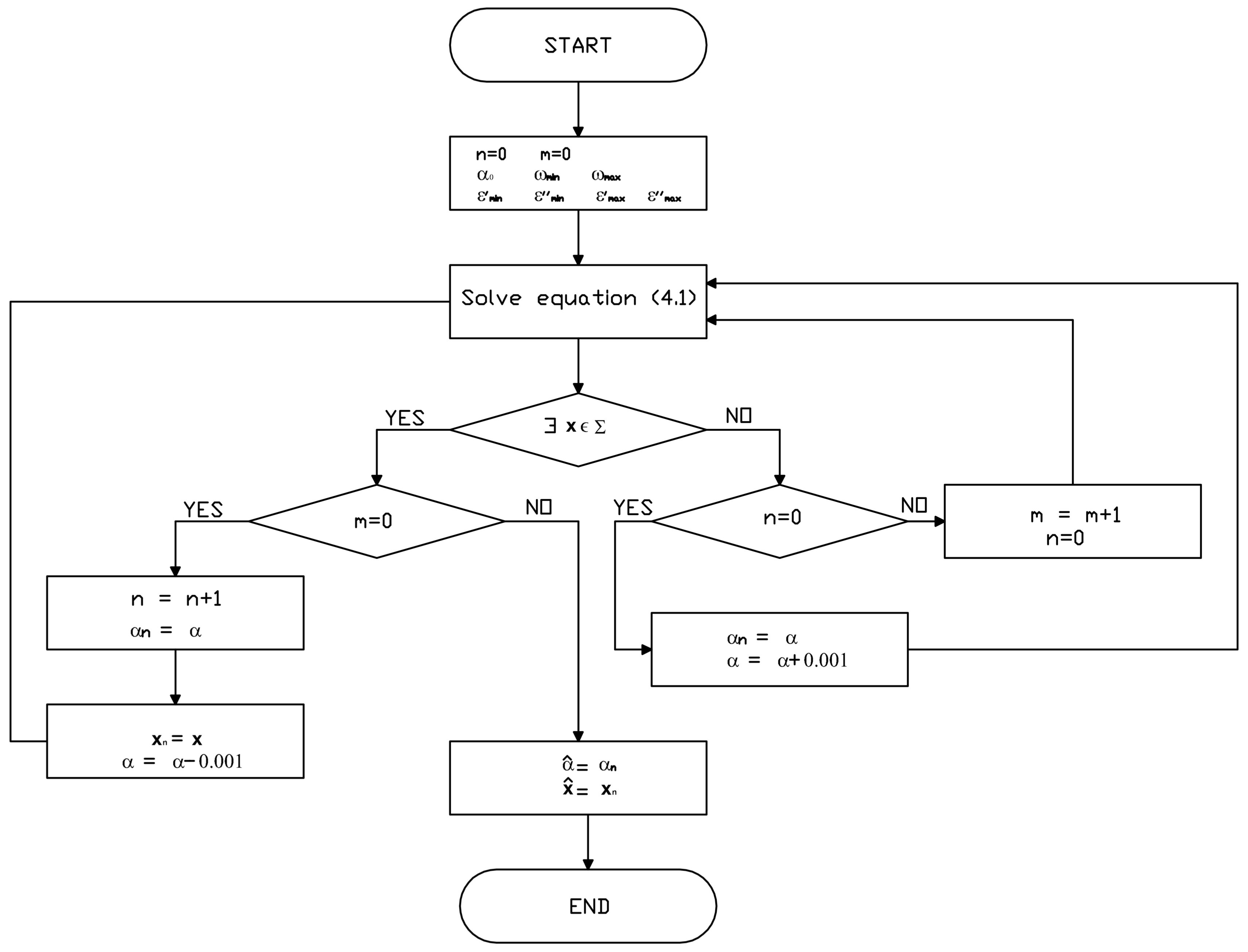
- Step 1
- one chooses a frequency range () and a test value for ;one read the correspondent permittivity experimental values:, , , ;one initializes and .
- Step 2
- one resolves the system at frequencies and .
- Step 3
- If there is a real and positive solution, then if m is not null go to end; otherwise, one puts:; ; ; ; ; ; ;it reduces = - 0.001 and go back to step 2.
- Step 4
- If n is null, one puts and = + 0.001 and go back to step 2; otherwise, one puts , and goes back to step 2.
- End
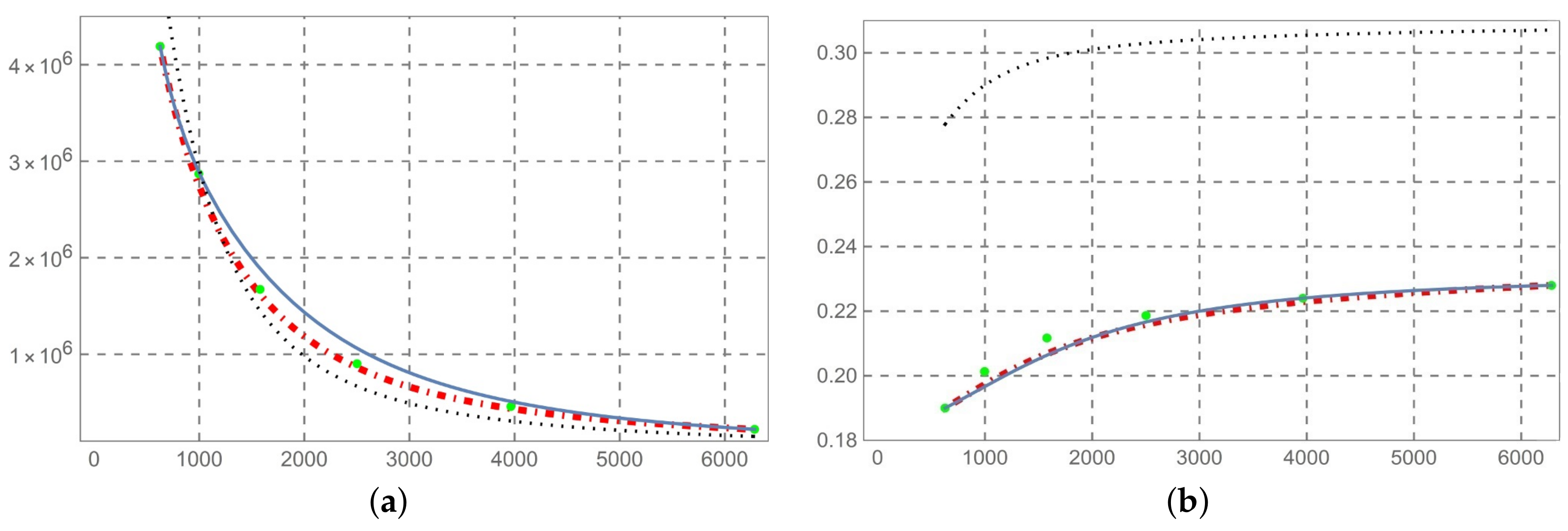
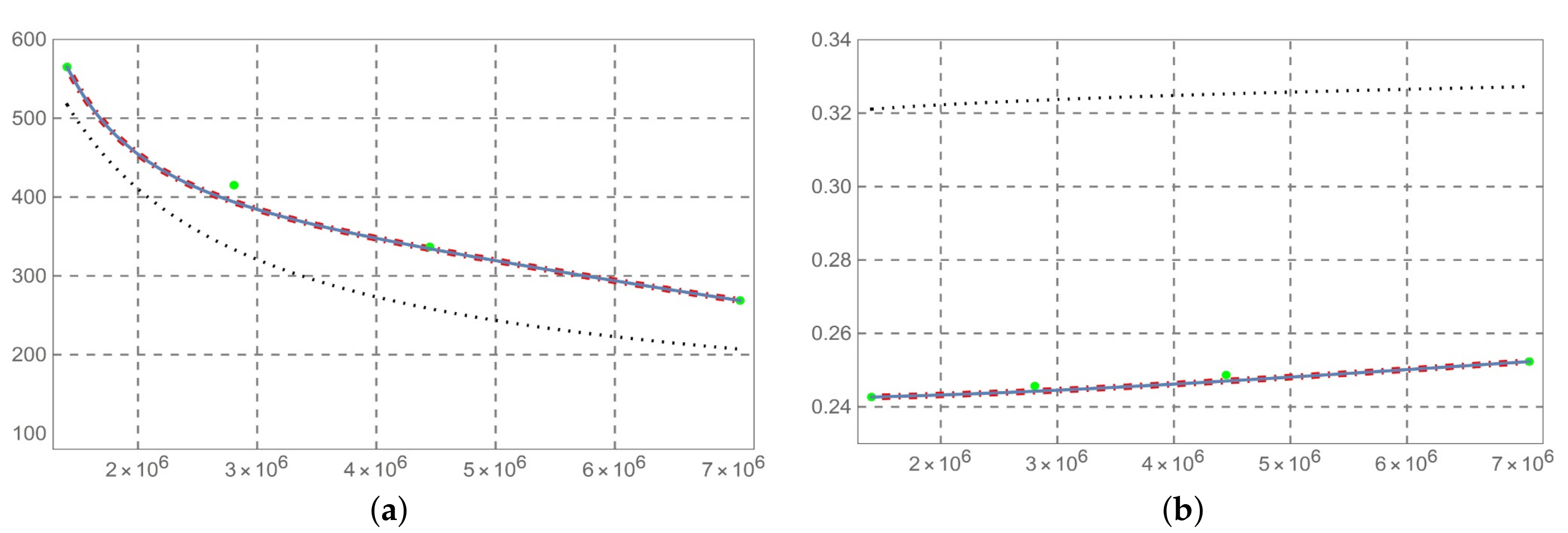
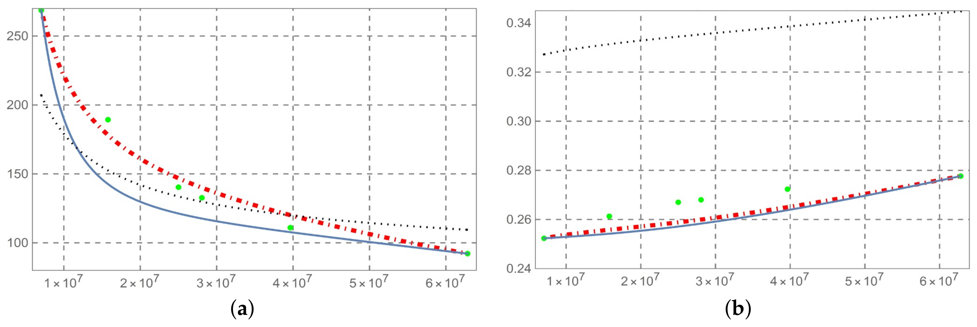
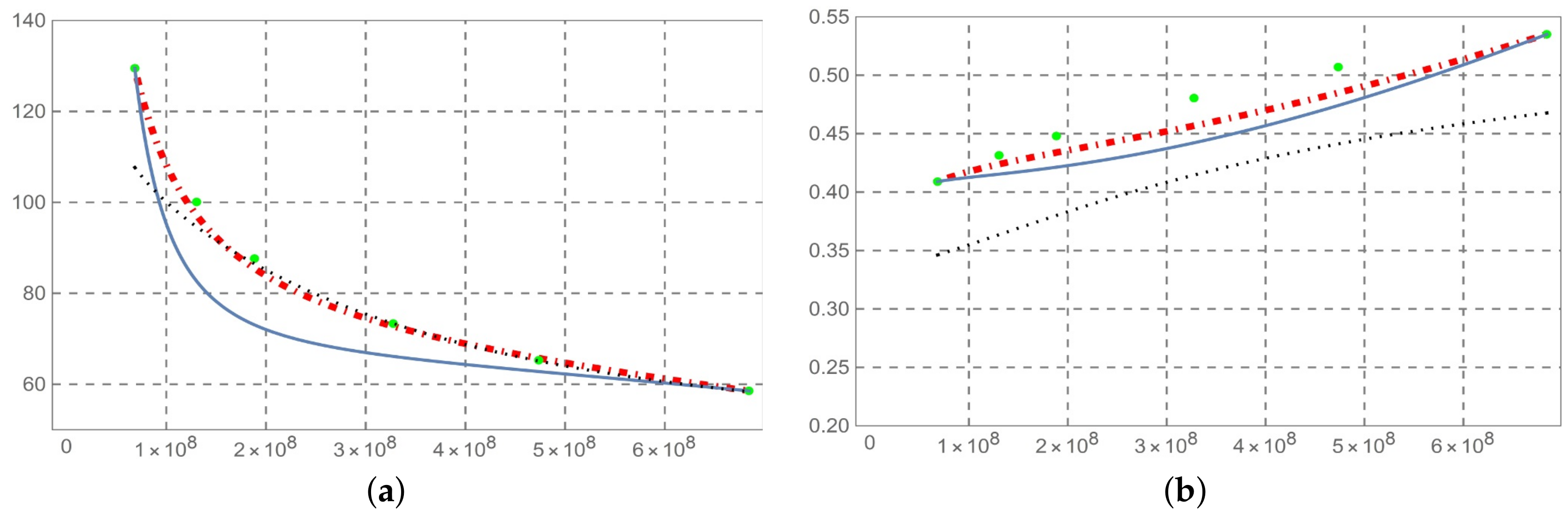
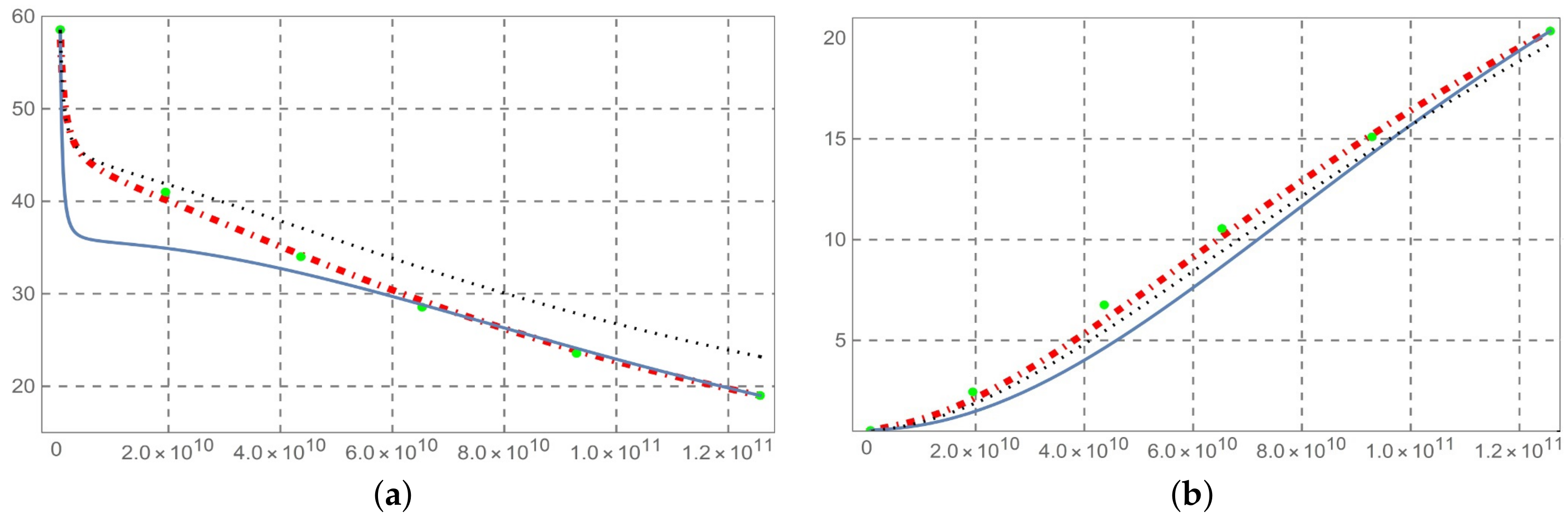
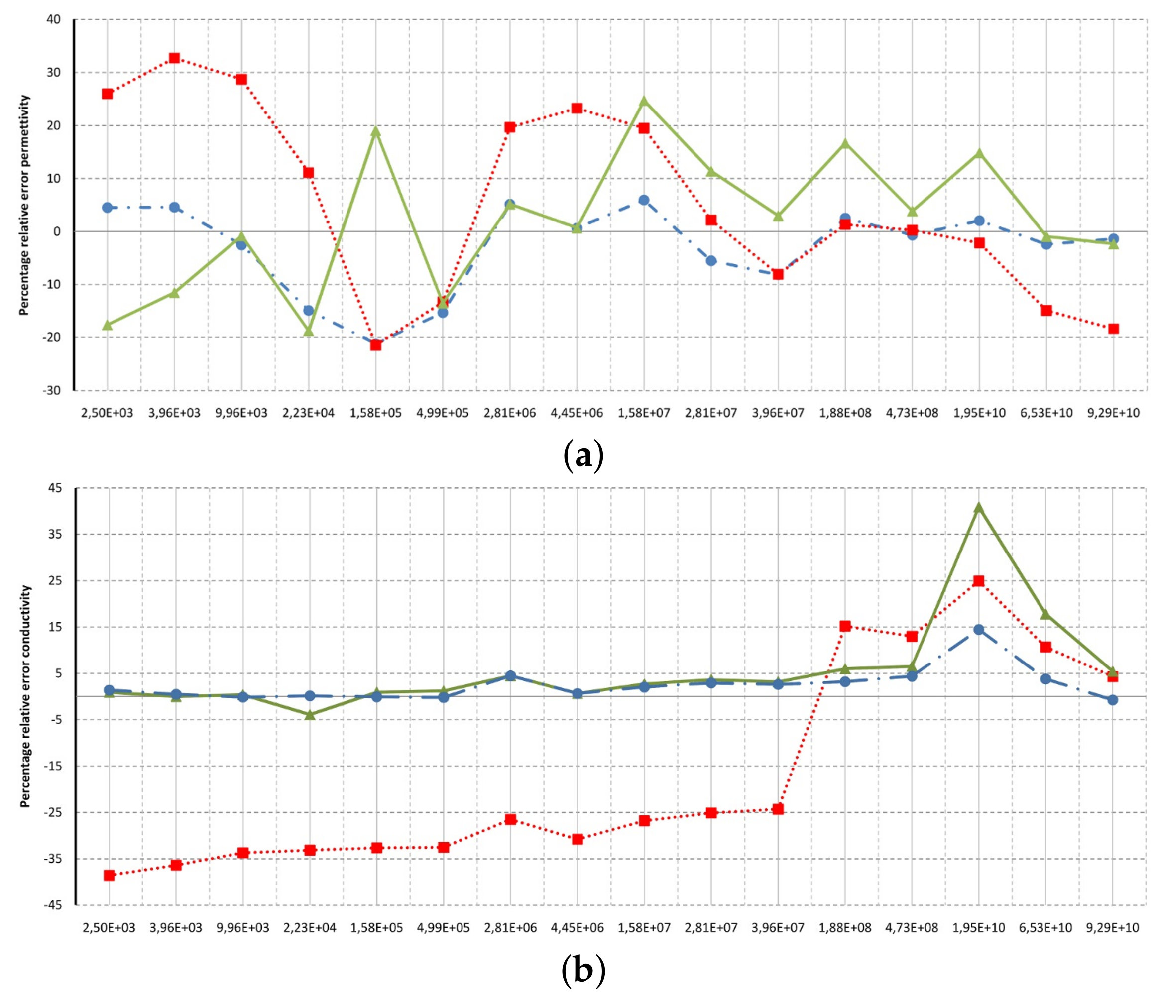
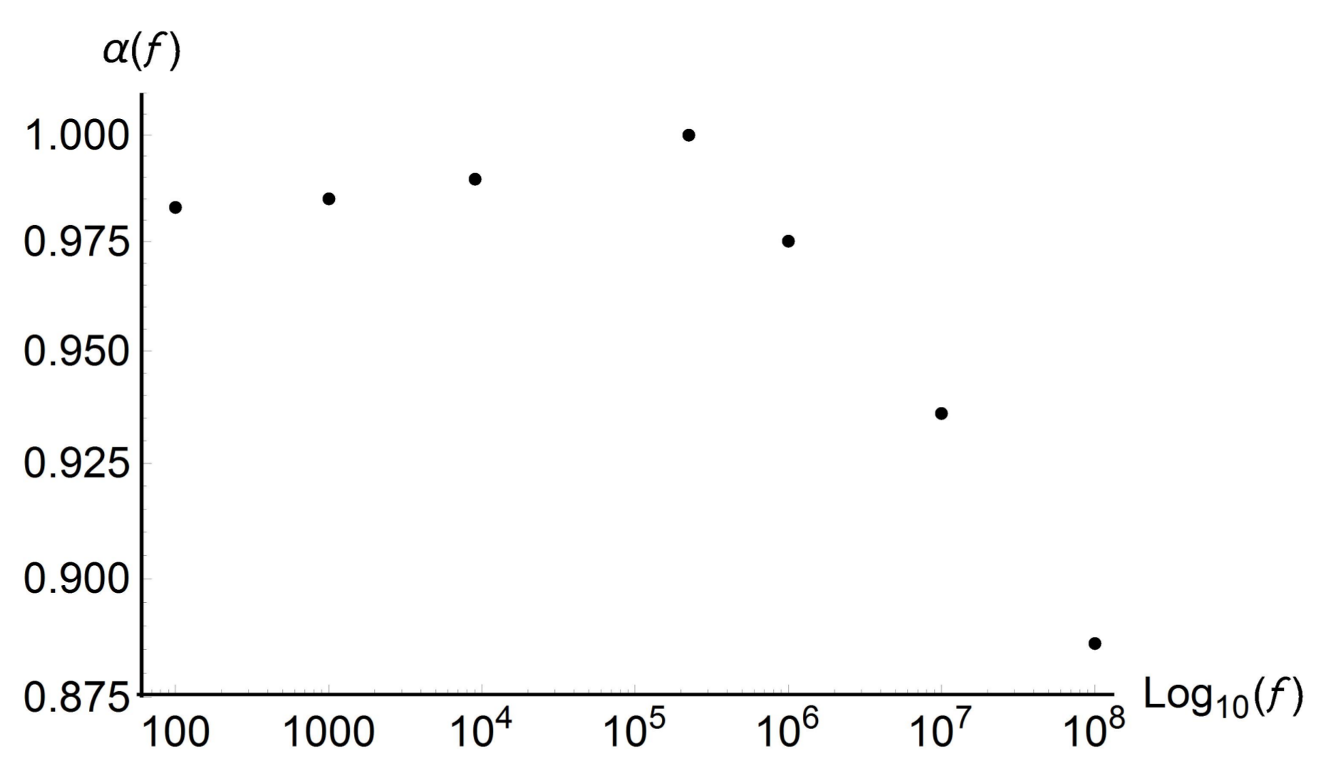
- The solution so determined is compared with the predictive permittivity model in [10], at a temperature of 37 °C with reference to the human aorta. This method is equally applicable to biological tissues. From Figure 2, Figure 3, Figure 4, Figure 5, Figure 6, Figure 7 and Figure 8 (horizontal axis rad/s), we observe that a predictive fractional model of the complex permittivity is in accordance with experimental data with good approximation. The experimental data are those relating to measure campaign published in [10]. In particular from Figure 9, we see that percentage error relative permittivity and conductivity to experimental data is, respectively, almost always lower and thorough than that of the Ciancio–Kluitenberg model and Cole–Cole extended model [7,8,9,10]. In the frequency range 2.5 × 10 @ 9.29 × 10, the maximum relative error to experimental data of permittivity fractional model is −21% at 1.58 × 10 rad/s; of Ciancio–Kluitenberg’s model is +25% at 1.58 × 10 rad/s and extended of Cole–Cole’s model is +35% at 1.58 × 10 rad/s; in the same frequency range, the maximum relative error to experimental data of conductivity fractional model is +15% at 1.95 × 10 rad/s; of Ciancio–Kluitenberg’s model is +41% at 1.95 × 10 rad/s and extended of Cole–Cole’s model is −37% at 2.5 × 10 rad/s. In Figure 10, we show the trend of fractional order with respect to the frequency.
5. Conclusions
It is emphasized that this fractional model derives from a physical theory that justifies the phenomenon of polarization on biological tissues. In particular, the Ciancio–Kluitenberg model has shown how the two time constants are related to strain and rotation of the cells that constitute the polarized biological tissue. Models like that of extended Cole–Cole are characterized by parameters whose values are empirically obtained i.e., without a justification of a physical nature. The transition to the fractional calculation was possible by replacing the ordinary derivative with Caputo’s fractional derivative to write the corresponding phenomenological equation of media with dielectric relaxation. From the complex permittivity model obtained, it has been seen (Figure 10) how the topology of the memory operator has fractional dimension frequency dependency and also that this tends to a minimum value in accordance with the 2nd Principle of Thermodynamics. The fractional model of the complex permittivity is in accordance with experimental data with good approximation. The reason why permittivity and conductivity deviates from experimental data at a given frequency ranges is not known, but this probably depends on the type of fractional derivative considered. A possible development of the proposed method is to determine the fixed fractional operator, the optimal fractional order functional with respect to frequency that minimizes the relative percentage error.
Acknowledgments
This paper was supported by National Group of Mathematical Physics GNFM-INdAM.
Author Contributions
These two authors contribute equally to this paper.
Conflicts of Interest
The authors declare no conflict of interest.
References
- Artis, F.; Chen, T.; Chretiennot, T.; Fournie, J.-J.; Poupot, M.; Dubuc, D.; Grenier, K. Microwaving biological cells. IEEE Microw. Mag. 2015, 16, 87–96. [Google Scholar] [CrossRef]
- Debye, P. Zur theorie der spezifischen Wärme. Ann. Phys. 1912, 39, 789–839. [Google Scholar] [CrossRef]
- Cole, K.S.; Cole, R.H. Dispersion and absorption in dielectrics I. Alternating current characteristics. J. Chem. Phys. 1941, 9, 341–349. [Google Scholar] [CrossRef]
- Cole, K.S.; Cole, R.H. Dispersion and absorption in dielectrics II. Direct current characteristics. J. Chem. Phys. 1942, 10, 98–105. [Google Scholar] [CrossRef]
- Davidson, D.W.; Cole, R.H. Dielectric relaxation in glycerol, propylene glycol, and n-propanol. J. Chem. Phys. 1951, 19, 1484–1490. [Google Scholar] [CrossRef]
- Havriliak, S.; Negami, S. A complex plane representation of dielectric and mechanical relaxation processes in some polymers. Polymer 1967, 8, 161–210. [Google Scholar] [CrossRef]
- Gabriel, S.; Lau, R.W.; Gabriel, C. The dielectric properties of biological tissues: I. Literature survey. Phys. Med. Biol. 1996, 41, 2231–2250. [Google Scholar] [CrossRef] [PubMed]
- Gabriel, S.; Lau, R.W.; Gabriel, C. The dielectric properties of biological tissues: II. Measurements in the frequency range 10 Hz to 20 GHz. Phys. Med. Biol. 1996, 41, 2251–2270. [Google Scholar] [CrossRef] [PubMed]
- Gabriel, S.; Lau, R.W.; Gabriel, C. The dielectric properties of biological tissues: III. Parametric models for the dielectric spectrum of tissues. Phys. Med. Biol. 1996, 41, 2271–2294. [Google Scholar] [CrossRef] [PubMed]
- Gabriel, C. Compilation of the Dielectric Properties of Body Tissues at RF and Microwave Frequencies; Amstrong Laboratory, Ed.; AFOSR/NL Bolling AFB DC 20332-0001; Report: N.AL/OE-TR-1996-0037; Brooks Air Force Base: San Antonio, TX, USA, 1996; pp. 1–272. [Google Scholar]
- Ciancio, V.; Kluitenberg, G.A. On electromagnetic waves in isotropic media with dielectric relaxation. Acta Phys. Hung. 1989, 66, 251–276. [Google Scholar] [CrossRef]
- Ciancio, V.; Farsaci, F.; Di Marco, G. A method for experimental evalutation of phenomenological coefficients in media with dielectric relaxation. Phys. B Condens. Matter 2007, 387, 130–135. [Google Scholar] [CrossRef]
- Ciancio, V.; Farsaci, F.; Rogolino, P. On a thermodynamical model for dielectric relaxation phenomena. Phys. B Condens. Matter 2010, 405, 175–179. [Google Scholar] [CrossRef]
- Kluitenberg, G.A. On vectorial internal variables and dielectric and magnetic relaxation phenomena. Phys. A Stat. Mech. Appl. 1981, 109, 91–122. [Google Scholar] [CrossRef]
- Caputo, M. Distributed order differential equations modelling dielectric induction and diffusion. Fract. Calc. Appl. Anal. 2001, 4, 421–442. [Google Scholar]
- Garrappa, R.; Mainardi, F.; Maione, G. Models of dielectric relaxation based on completely monotone functions. Fract. Calc. Appl. Anal. 2016, 19, 1105–1160. [Google Scholar] [CrossRef]
- Kiryakova, V. A brief story about the operators of generalized fractional calculus. Fract. Calc. Appl. Anal. 2008, 11, 201–218. [Google Scholar]
- Caputo, M.; Fabrizio, M. Applications of New Time and Spatial Fractional Derivatives with Exponential Kernels. PFDA 2016, 2, 1–11. [Google Scholar] [CrossRef]
- Caputo, M.; Fabrizio, M. A new definition of fractional derivative without singular kernel. PFDA 2015, 1, 73–85. [Google Scholar] [CrossRef]
- Ciancio, V.; Flora, B.F.F. Technical Note on a New Definition of Fractional Derivative. PFDA 2017, 3, 1–4. [Google Scholar] [CrossRef]
- Caputo, M.; Fabrizio, M. Admissible frequency domain response functions of dielectrics. Math. Meth. Appl. Sci. 2015, 38, 930–936. [Google Scholar] [CrossRef]
Figure 1.
Flow-chart.

Figure 2.
(a) Permittivity and (b) conductivity at frequencies 100 Hz @ 1 KHz. Line dot-dashed fractional model , line continue ordinary model, line dotted extensive Cole–Cole’s model, points experimental data.
Figure 2.
(a) Permittivity and (b) conductivity at frequencies 100 Hz @ 1 KHz. Line dot-dashed fractional model , line continue ordinary model, line dotted extensive Cole–Cole’s model, points experimental data.

Figure 3.
(a) Permittivity and (b) conductivity at frequencies 1 KHz @ 9 KHz. Line dot-dashed fractional model , line continue ordinary model, line dotted extensive Cole–Cole’s model, points experimental data.
Figure 3.
(a) Permittivity and (b) conductivity at frequencies 1 KHz @ 9 KHz. Line dot-dashed fractional model , line continue ordinary model, line dotted extensive Cole–Cole’s model, points experimental data.

Figure 4.
(a) Permittivity and (b) conductivity at frequencies 9 KHz @ 224 KHz. Line dot-dashed fractional model , line continue ordinary model, line dotted extensive Cole–Cole’s model, points experimental data.
Figure 4.
(a) Permittivity and (b) conductivity at frequencies 9 KHz @ 224 KHz. Line dot-dashed fractional model , line continue ordinary model, line dotted extensive Cole–Cole’s model, points experimental data.
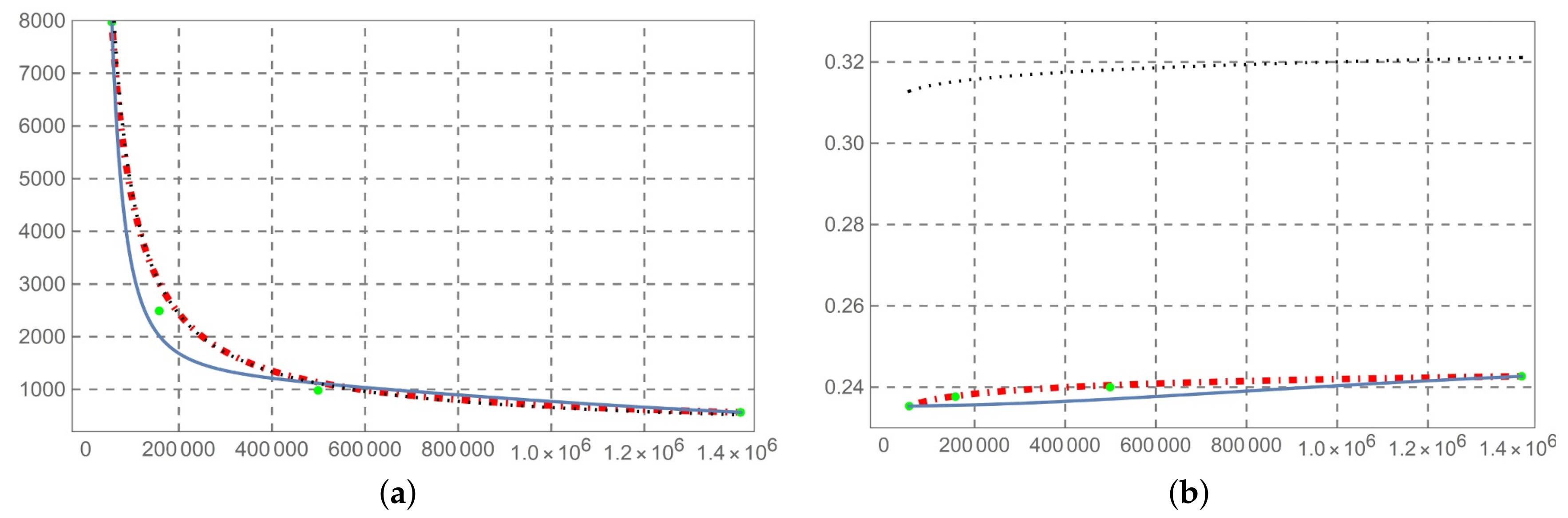
Figure 5.
(a) Permittivity and (b) conductivity at frequencies . Line dot-dashed fractional model , line continue ordinary model, line dotted extensive Cole–Cole’s model, points experimental data.
Figure 5.
(a) Permittivity and (b) conductivity at frequencies . Line dot-dashed fractional model , line continue ordinary model, line dotted extensive Cole–Cole’s model, points experimental data.

Figure 6.
(a) Permittivity and (b) conductivity at frequencies 1 MHz @ 10 MHz. Line dot-dashed fractional model , line continue ordinary model, line dotted extensive Cole–Cole’s model, points experimental data.
Figure 6.
(a) Permittivity and (b) conductivity at frequencies 1 MHz @ 10 MHz. Line dot-dashed fractional model , line continue ordinary model, line dotted extensive Cole–Cole’s model, points experimental data.

Figure 7.
(a) Permittivity and (b) conductivity at frequencies 10 MHz @ 100 MHz. Line dot-dashed fractional model , line continue ordinary model, line dotted extensive Cole–Cole’s model, points experimental data.
Figure 7.
(a) Permittivity and (b) conductivity at frequencies 10 MHz @ 100 MHz. Line dot-dashed fractional model , line continue ordinary model, line dotted extensive Cole–Cole’s model, points experimental data.

Figure 8.
(a) Permittivity and (b) conductivity 100 MHz @ 20 GHz. Line dot-dashed fractional model , line continue ordinary model, line dotted extensive Cole–Cole’s model, points experimental data.
Figure 8.
(a) Permittivity and (b) conductivity 100 MHz @ 20 GHz. Line dot-dashed fractional model , line continue ordinary model, line dotted extensive Cole–Cole’s model, points experimental data.

Figure 9.
Relative percentage error (a) permittivity and (b) conductivity. Line dot-dashed fractional model, line continue Ciancio–Kluitenberg model, line dotted extensive Cole–Cole’s model, points experimental data.
Figure 9.
Relative percentage error (a) permittivity and (b) conductivity. Line dot-dashed fractional model, line continue Ciancio–Kluitenberg model, line dotted extensive Cole–Cole’s model, points experimental data.

Figure 10.
Trend fractional order respect to frequency.
© 2017 by the authors. Licensee MDPI, Basel, Switzerland. This article is an open access article distributed under the terms and conditions of the Creative Commons Attribution (CC BY) license (http://creativecommons.org/licenses/by/4.0/).
Share and Cite
MDPI and ACS Style
Ciancio, A.; Flora, B.F.F. A Fractional Complex Permittivity Model of Media with Dielectric Relaxation. Fractal Fract. 2017, 1, 4. https://doi.org/10.3390/fractalfract1010004
AMA Style
Ciancio A, Flora BFF. A Fractional Complex Permittivity Model of Media with Dielectric Relaxation. Fractal and Fractional. 2017; 1(1):4. https://doi.org/10.3390/fractalfract1010004
Chicago/Turabian StyleCiancio, Armando, and Bruno Felice Filippo Flora. 2017. "A Fractional Complex Permittivity Model of Media with Dielectric Relaxation" Fractal and Fractional 1, no. 1: 4. https://doi.org/10.3390/fractalfract1010004