Fractional Divergence of Probability Densities

P.O. Box 123AA, Adelaide, SA 5000, Australia
Fractal Fract. 2017, 1(1), 8; https://doi.org/10.3390/fractalfract1010008
Submission received: 12 September 2017
/
Revised: 18 October 2017
/
Accepted: 19 October 2017
/
Published: 25 October 2017
Abstract
:The divergence or relative entropy between probability densities is examined. Solutions that minimise the divergence between two distributions are usually “trivial” or unique. By using a fractional-order formulation for the divergence with respect to the parameters, the distance between probability densities can be minimised so that multiple non-trivial solutions can be obtained. As a result, the fractional divergence approach reduces the divergence to zero even when this is not possible via the conventional method. This allows replacement of a more complicated probability density with one that has a simpler mathematical form for more general cases.
1. Introduction
The divergence or relative entropy between two probability densities is a measure of dissimilarity between them. The most well known divergence approach is due to Kullback and Leibler which will be discussed in more detail below. Other divergence formulations include the version by Jeffrey which is symmetric for large separations between densities [1]. While Jeffrey’s approach is a symmetric f-divergence and is non-negative, it does not obey the triangle inequality. The Jensen–Shannon divergence [2] is essentially a half times the sum of the two separate densities and their respective divergence to their mean. The striking feature about the Jensen–Shannon divergence is that its square root is a true distance metric. That is, it not only displays symmetry but also conforms to the triangle inequality. Closely related to the divergence or relative entropy is entropy itself. Some of the definitions are due to Renyi [3], a one-parameter generalisation of the Shannon entropy and the definition due to Tsallis [4]. Tsallis entropy is in fact the underlying formulation for many other entropy definitions in the literature.
There have been attempts to generalise the concepts of divergence and entropy using fractional calculus. Fractional order mathematics has been applied to many classical areas associated with probability, entropy and divergence. The entropy has been derived in fractional form in [5] and subsequently in [6]. Divergence measures based on the Shannon entropy have been dealt with in [7]. An interpretation of fractional order differentiation in the context of probability has been given in [8]. The role of fractional calculus in probability has been discussed in [9]. In [10], the connection of fractional derivatives and negative probability densities is discussed. One of the first attempts to involve fractional calculus with probability theory is due to Jumarie [11]. The fractional probability measure is discussed, in particular the uniform probability density of fractional order. Comparison of the properties of fractional probabilities to the properties of classical probability theory have been studied in [12,13,14]. These latter works extend the ideas of Jumarie and give definitions for fractional probability space and fractional probability measure so that a fractional analogue of the classical probability theory is obtained.
The underlying mathematical construct in all of these approaches is the dependence on probability densities or distributions. In many areas of research, there is a requirement to model the statistical behaviour of a physical process by using probability distributions in terms of the cumulative distribution function (CDF) or the probability density function (PDF). Depending on the problem to be analysed, there is usually a particular distribution that is better suited for the description of the physical process compared to other distributions. The problem is that most distributions contain multiple parameters that must be estimated using such methods as the maximum likelihood approach or method of moments. The estimation of these parameters introduces uncertainty, which translates to performance loss for a particular distribution when used to model physical phenomena. For example, in the detection of signals using the Constant False Alarm Rate (CFAR) approach [15,16,17,18,19], correct estimation of parameters is critical. The estimation of these parameters is almost always not exact and, as a consequence, the detection performance drops because of the loss in accuracy.
The basic requirement is to find a probability density that describes a physical process accurately while possessing a smaller number of parameters. In other words, is there a simpler probability density that can replace a more complicated two or more parameter version? This means that the simpler expression must match the performance of the latter very well for a large solution set. The use of a separation metric is required that will indicate how dissimilar they are. If the separation between them is zero or very close to zero, then the more complicated density can be replaced by the “simpler” density (or approximation). Much work has been done on this problem and two methods have proven to be very useful. The first involves information geometry [20] where the separation is given by the geodesic distance between two probability density-manifolds. The geodesic is obtained via the Fisher–Rao information metric. The geodesic is a true metric because it is symmetric between the densities and obeys the triangle inequality.
The other approach is to consider a class of divergence formulations called f-divergences of which the Kullback–Leibler version belongs to. The Kullback–Leibler divergence is not symmetric for large separations between densities and does not obey the triangle inequality. However, there are a number of ways to make it symmetric for large separations between densities. It is worth noting that there is a mathematical duality between the Kullback–Leibler divergence and the geodesic approach of information geometry. In addition, the latter is more complicated to work with in the mathematical sense because, in many cases, the geodesic must be obtained via the solution of partial differential equations. On the other hand, an f-divergence formulation such as the Kullback–Leibler divergence is relatively easier to implement, requiring the solutions to be obtained via integrals instead.
The Kullback–Leibler divergence has been used previously to find solutions that allow one density or model to be replaced by another [21,22,23,24,25,26,27,28,29]. The problem is that the solution sets that give a divergence of zero or close to zero are either unique or trivial in nature. That is, the divergence is not valid for a large set of parameter values. Replacing one model (density) by another only for certain unique or restricted values in their parameters is not very useful for modelling physical processes or systems. Unfortunately, this is the inherent problem associated with the current form of any divergence method. What is required is an approach that extends the solutions, where the divergence is close to zero or zero, beyond the unique and trivial cases. It would then be possible to replace one model with another since there would be a similarity between them for large parameter sets. This idea will be pursued in this paper by making use of fractional calculus to obtain a fractional form for the Kullback–Leibler divergence.
2. Divergence between Two Probability Densities
The divergence between two probability densities considered here is based on the Kullback–Leibler formulation (K-L). This is a pseudo-metric for the distance between the densities because it fails the triangle inequality. The main issue with the K-L formulation is that it is not symmetric unless the metric separation between the densities is small, i.e., probability density is very close in parameter space to density : , where is the parameter space of each density and N represents the total number of parameters. The K-L divergence is defined as
for some region of integration . It is possible to obtain a symmetric version of (1) that is valid for larger separations and obeys the triangle inequality. One way to do this is using the Jeffrey’s formulation as discussed previously:
It will suffice to consider the divergence as given by (1) in what follows since the approach discussed in this paper is easily applicable to the symmetric Jeffrey’s case or other similar formulations. Either way, this does not matter much, since, for almost all cases of interest, small separations dominate. The K–L divergence (1), hereby referred to as the divergence for brevity, is also known as the relative entropy for the following reason. If (1) is re-written as
then the negative of the first integral in (3) is the differential entropy H of the probability density . It was first used in statistical physics by Boltzmann and in information theory by Shannon. Both considered the discreet form for a probability mass
The integral with a positive sign on the right of (3) is the cross-entropy between the densities and . Hence, (1) and (3) are also referred to as the relative entropy between two densities. The divergence or relative entropy between probability densities and are interpreted in the following sense. Assume that a physical process or system is known to be accurately represented and modelled by a probability density . This density might also represent an ideal or theoretical model. Is there another (perhaps simpler) model with density that is asymptotically close or exact with the former density (model)? If the two densities have a divergence that tends to zero, then the more complicated model can be replaced by the simpler model (approximation) for the given parameters that achieve zero or almost zero divergence. In another sense, the way to understand this is to ask what information is lost if one used the model density compared to the more accurate model density . As an example, use of divergence in signal processing is very important—in particular, the detection of targets amongst background noise and clutter. This requires determining if signals (targets) of a given probability density differ from another density that represents the background noise and clutter. The degree of separation above a given threshold determines whether targets are present or not (see Section 6). In fact, the concept of divergence is used in many areas of physics, statistics/mathematics and engineering with a common goal. Ideally, the requirement is to find solutions to (1) in terms of the parameter vectors and that make the divergence equal to zero, i.e.,
or from (3) when the entropy term is equal to the cross entropy term. The problem is, since the two densities are different and with different parameters, it is not possible to achieve zero divergence between them except perhaps for particular or unique solutions such as solutions pertaining to their intersections. In some cases, the solutions are trivial such as when the two densities are of the exact mathematical form, which means a divergence of zero is possible since the parameters of one can be made to take on the same values as those of the other. For example, for two Exponential densities with parameters and , it is trivial to show by inspection or by using the divergence (1) that
have a divergence of zero everywhere only when . In fact, forcing the divergence to be zero as in (5) may not necessarily give solutions that achieve zero divergence. In such cases, it is also possible that the solutions become complex, which does not make sense when applied to a real physical problem. In what follows, it will be shown that it is possible to extend the domain of validity of solutions that give zero divergence beyond the trivial or unique cases. This can be done via the transformation of one or more of the parameters appearing in the divergence equations using fractional calculus. The method will be applied to two important densities used in many fields of research: the Exponential density and a well known power form, namely, the Pareto density. The first step is to obtain the conventional and fractional divergences for the Exponential-Pareto case and then to do the same for the Exponential–Exponential case.
3. Conventional Divergence of Exponential and Pareto Densities
The Exponential and Pareto distributions have been used to model a large number of problems. For example, the Pareto distribution is critical in the analysis of radar clutter. For this reason, a fractional-order Pareto distribution has been presented in [30] in order to more accurately model sea clutter in microwave radar. Consider random variables belonging to the Exponential density as well as the Pareto density . That is,
where the parameter space contains only one parameter, , which is usually related to the expectation of the random variables by . The Pareto density has parameter space where is the scale parameter and is the shape parameter:
The idea here is to replace the two parameter Pareto density with the one parameter and simpler Exponential density. On this basis, this can only be true for certain solutions where the divergence between them is zero or close to zero. For brevity, the densities will be written as and . The divergence expression between the Exponential and Pareto densities is obtained from
where the log-function in the integrand is simplified to
Substituting into (9) and taking the integration domain to be the interval , the divergence now becomes,
The first term in the integrand is trivial since the second axiom of probability states that the integral of the density in the interval is unity: . The other terms can be completed by using integration by parts to finally arrive at the following expression for the divergence between the two densities
where the Euler-gamma has been introduced and its value is . The modulus is included in (12) to enforce the fact that the divergence is greater or equal to zero. The idea now is to work out for what values of in (12) the divergence approaches zero. That is, what values of make the Pareto density be approximate to or become equal to the Exponential respectively? Let the parameter space of all parameters be written as a vector . Consider the derivative as an operator . Taking the index gives the operator in terms of the parameter , i.e., . Using the operator on the left and right of (12) gives, (ignoring the modulus):
where . We enforce the need for the left-hand side to be equal to zero as required, i.e., so that
Solving for :
This means that the density has a divergence that is zero or close to zero with respect to , the Exponential, whenever is given by (15). Then, the Pareto density is modified to
The Pareto density (16) is now expressed in terms of the Exponential-density parameter . This indicates where the divergence of from is approaching zero as a function of . When the divergence is acceptably small or even zero, the Pareto model can be adequately described by the simpler one-parameter Exponential model. Thus, substituting (15) into (12) means that the divergence can be written as:
where . Equation (17) determines the value of the minimum-divergence between the two densities. Figure 1 shows a plot of the divergence (17) as a function of the parameter at . The conventional divergence (17) is zero for the unique value of in the range considered. Multiple solutions that approach zero are not generally possible. In this case, the divergence between the densities and is zero only for the particular value and close to zero for small values of on either side.
In fact, for the general case, the conventional divergence given by the expression (12) can be plotted as a function of the parameters . Figure 2a shows the divergence between the two densities as a function of the two parameters and at a fixed Pareto scale parameter value of . For the range of and values shown, the divergence is never zero or very close to zero. In terms of Figure 1, the divergence is zero for and this occurs when , which is outside the range of values for shown in Figure 2a. An exact divergence of zero at only one unique point is not very useful or practical in the general sense anyway. What is required is an extension of the solutions so that zero divergence (or very close to zero) is achieved over a wider parameter range (see Figure 2b). This will require the use of fractional-order calculus and will be discussed in the next section.
4. Fractional Divergence of Exponential and Pareto Densities
Fractional calculus has been around since the time of integer order calculus, which was developed by Newton and Leibniz. The name “fractional” is a misnomer that has endured since around 1695 when l’ Hopital queried Leibniz on the meaning of a fractional order of one-half for the derivative operator. It is to be understood that fractional really means “generalised”. Fractional-order derivatives and integrals of functions have been studied for a very long time with various definitions appearing in the literature. Among the well known are due to Caputo, Grunwald-Letnikov and Riemann–Liouville. For a comprehensive review of the many versions that have been derived, see [31] and the references therein. Research into fractional order mathematics has been prevalent in recent times in many fields of science, mathematics and engineering [32,33,34,35,36,37,38,39,40,41]. In this paper, the interest is in the fractional derivative of functions only and the Riemann–Liouville formulation for the fractional derivative will be considered:
The terminal a takes two values. The case is due to Liouville while the case is due to Riemann. The parameter represents values that are integer order, i.e., . The parameter is the fractional order that can be real or complex and is bounded by . Here, is the floor function and is the ceiling function, respectively. Consider the Riemann–Liouville fractional derivative for and terminal . The following fractional operator can then be defined:
Applying the operator on the conventional divergence, i.e., , gives the fractional divergence such that the following holds:
Definition 1.
The fractional divergence, which is a generalisation of the conventional divergence, is defined as
where is the expectation with respect to the density and the three axioms of probability theory hold for both densities. The modulus is required because and . In addition, the definition: whenever is applicable.
Theorem 1.
If the fractional divergence is a generalised form for the divergence between two densities, it must produce the same solutions as the conventional divergence as a special limit. The latter is true when the fractional order approaches in (20). Thus,
or in operator form:
Proof.
The proof involves showing that the fractional operator of order, , reduces to the -th integer order derivative in the limit . The final stage requires setting to complete the proof. Let be an arbitrary integer order of the conventional derivative. Let the fractional order operator be written in terms of the integer order derivative ,
where the expression on the right is obtained by using the transformation . Then,
The conventional divergence corresponds to the integer order , hence
as required. Note that the mapping has been applied in (25). ☐
The divergence integral appearing in the integrand of (20), i.e., the expectation, has already been calculated before (see (12)). The parameter vector space for both densities is . Re-arranging the divergence expression (12), the following form is obtained, (neglecting the modulus until the end):
where and have been omitted for brevity. The requirement now is to use the operator and calculate the fractional divergence as follows:
The argument implies that the variable x maps on to the variable . This will be elucidated further in what follows below. Recall that the parameter vector is given by and as before, in Section 3, the interest is in the parameter , i.e., so that . In addition, the condition is enforced so that (27) becomes
Each term appearing in (28) will now be calculated. Before proceeding, it is important to re-visit the meaning of the mapping . Once the operator is used, the final result is a function of the variable x, which must then be replaced by the variable , i.e, . The first term in (28) will be calculated last as it is more involved than the other two. In addition, the function , for some argument z, always appears in these kinds of problems involving divergence or parameter estimation, and, for this reason, it will be treated in full. The other two terms contain monomials and . It can be shown, by using the Riemann–Liouville fractional formulation, that the fractional derivative of monomials with power n results in a form that is the exact version of Euler’s generalisation of the integer derivatives of monomials:
for monomial powers n. To verify this, the second term is (leaving out the coefficient):
Let the above integral be transformed to the form
using the transformation and . The requirement now is to map the variable x such that in (31) to obtain the final result
since . As stated above, this result is equivalent to that obtained by using Euler’s form (29) for . In a similar way, the final term in (28) can be obtained as follows (leaving out the coefficient again),
where the transformation and have been applied. The final result then becomes:
Once again, this result can be obtained directly from the Euler Equation (29) for . The first term of (28) is now evaluated as follows:
To perform the integration in (35), let so that and this gives
where has been used in (36) to expand the integrand. The first integral on the right of (36) is only dependent on the variable y so that it is trivial to show that
The second integral in (36) can be solved if so that and the integral becomes,
Here, is the harmonic-function that is related to the polygamma-function of the zeroth order or digamma-function via , where is the Euler gamma constant. The digamma-function can be simplified further by using the identity:
Setting and in the identity, one obtains . Hence, (38) can be re-written as:
After performing the simple differentiation in (41) and noting that we have:
The problem now requires the solution of (43) in terms of the parameter , which will be the fractional analogue of the conventional version as discussed in Section 3. Unfortunately, due to the fact that (43) is a transcendental equation in , it means that solutions can only be obtained numerically. However it is possible to rewrite (43) in such a way as to obtain closed form analytic solutions. Equation (43) can be re-arranged to:
Define A and B as follows:
so that (44) becomes:
which allows the solution in terms of to be in closed form if it can be transformed to resemble the Lambert W-function or product-log function. The W-function has the form
That is, if any equation can be written so that the left-hand side resembles the left-hand side of (47), then for any function on the right side, , the solution for y is given by: , where are the two branch cuts of the Lambert W-function. Equation (46) can now be solved via the W-function if it is transposed as follows:
Substituting both A and B while noting that gives the fractional as:
where the argument of the W-function, is
and the branch cut is considered for the W-function. The fractional form for the Pareto shape parameter, (50), can now be substituted into the conventional Pareto to obtain the fractional Pareto density (PDF) that minimizes the divergence with respect to the Exponential-density:
This is the fractional analogue of (16). Equation (50) can be substituted into the divergence Equation (12) as was done for the conventional solution for (see (15)). Thus, the fractional divergence becomes:
The modulus in (53) has been reinstated not only to ensure a divergence greater or equal to zero but also because the fractional order can take, not just real, but also complex values. The interesting aspect of the fractional order appearing in (51) and (53) is that the fractional now depends on (see (50)). There is no reason why the fractional order cannot be replaced by the variable . This means of course that takes on the same domain or range of values that does so defining the correct range is critical. In this instance, using (51) and (53) is essentially the same as using the following forms. Set to obtain:
and
Thus, in keeping with the conventional divergence plot shown in Figure 2a, Figure 2b shows a plot of the fractional divergence (55) (or (53)) for the parameters and . As can be seen from the color bars, the divergence is large for the conventional divergence. However, the fractional version shows not only much smaller divergence separations for various values of and , but a large region where the divergence is everywhere equal to zero. It is worth noting that the minimum divergence achieved by the conventional divergence is , which is still much greater than the maximum fractional divergence of .
5. Manipulation of the Divergence between Two Exponential Densities via the Fractional Orders
The fractional divergence between two Exponential-densities will be investigated in this section with the aim of showing that it gives non-trivial solutions and that it is possible to manipulate the divergence via the fractional order(s). There is a good reason for analysing two Exponential-densities as opposed to any other densities. Unlike the divergence solutions obtained for arbitrary densities, which are not entirely known, there is absolute certainty as to the expected divergence profile for the Exponential-densities. This is because, according to the conventional divergence, there is zero divergence whenever their parameters are equal. There are no other solutions that minimise the divergence for two Exponential-densities. Let
be two Exponential-densities. The two Exponential-densities (56) have one parameter each so that and . This corresponds to respectively. Omitting the modulus for now, the expression for the fractional divergence becomes,
The following two equations are obtained from (57):
when and
when . The domain of integration for the two densities is . The conventional divergence which is embedded in (58) and (59), is evaluated as follows:
The first terms in (60) is straightforward since the second axiom of probability applies, while the second term requires integration by parts. The conventional divergence between two Exponential-densities takes the form:
Using the operator form and enforcing the condition means that the fractional divergence with respect to parameter u becomes
Applying the fractional operator on the function has been addressed in the previous section. The result here follows a similar process that gives:
Once again, is the digamma function and is the Euler constant. The next term is evaluated to give the result:
The final requirement is to evaluate the ratio . Application of the fractional operator on this ratio gives the result:
Equation (67) can only be solved numerically for u in its present form. However, as shown in the previous section, it can be transformed so that its solutions can be obtained analytically by using the Lambert W-function. Setting
requires the solution of u using the form
Transforming this expression to a form that allows solution using the W-function finally gives (see previous section):
The solution (70) is a function of the fractional order as well as other parameters. The fractional order belonging to u will be distinguished from now on and will be defined as . The same will be done later for the solution v, which will be a function of its own fractional order . Hence, substituting (68) into (70), the final result becomes:
where the argument in the W-function is given by,
The next step is to complete a similar process for the parameter v. Substitution of the conventional divergence (61) into (59) requires the solution of
Using the operator formulation, and noting that , gives the expression:
Each term is now evaluated beginning with the first term:
The next term involves the log-function, which has been treated before in detail. Following the same process gives:
where once again is the digamma-function and is the Euler constant. The final term is evaluated to be:
It is now a matter of substituting (75)–(77) into (74). Rearranging the expression gives the following form:
In order to solve this equation using the W-function, set
The required equation takes the form
Rearranging this equation into the form that allows a solution by the W-function finally gives
As was done for the u-solution, the fractional order of v will be set to to distinguish it from belonging to the parameter u. With this in mind and substituting the definitions for A and B, namely (79), gives
where
The conventional divergence can now be transformed to the fractional divergence between two Exponential-densities by substituting the fractional solutions (71)–(72) for u and (82)–(83) for v into (61) to obtain the final form:
where the arguments and are given by:
The modulus is used because as well as as can be seen from (84) and (85). In Figure 3, the conventional divergence, which is exact with the fractional divergence when in the latter, is shown as a divergence manifold (top-left) with the line running down the middle where the divergence is zero.
The conventional divergence is also shown on the right as an image map where the red region indicates small divergence on either side of the line (not shown). According to the conventional divergence between two Exponential-densities, the only solutions which give zero are those where . However, as the middle two and last two plots indicate, the fractional divergence can make the divergence between them zero or close to zero for regions (solutions) where the conventional version fails. The middle two figures show manipulation of the divergence manifold for and in which the divergence manifold has been minimised perpendicular to the conventional version (). The image map on the right also contains iteration lines with each point being an iteration step in the process of finding the global minimum of the divergence using a differential-evolution numerical algorithm. This minimum occurs when and and at those parametric coordinates the fractional divergence is . The bottom two plots show further manipulation of the divergence manifold for giving a fractional divergence of for a global minimum in this case given by and . The last four plots confirm that the fractional divergence approach can give essentially zero divergence for parameter values which are not equal, unlike the expected results from the conventional divergence approach.
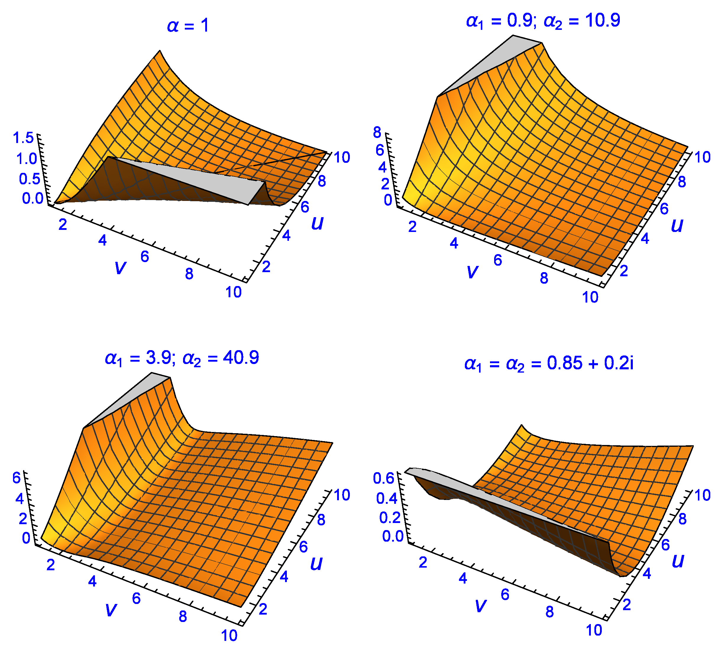
Further evidence of this can be seen in Figure 4. The manipulation of the divergence manifold is not only possible via but also when and are complex (bottom-right plot). The fractional divergence has a global minimum for the complex solution of at . There are numerous other non-trivial solutions with divergence of the order of or less which have been omitted for brevity reasons. The results shown in Figure 3 and Figure 4 indicate that the fractional divergence formulation makes it possible to find parameter values that achieve zero divergence even when the conventional approach does not. When the fractional order is , the fractional divergence recovers the same ‘trivial’ solutions as the conventional method, hence the former is a generalisation of the latter. Note that one can set or or any combination, where and .
Finally, it is worth discussing the or conventional divergence image map on the right of Figure 3. At first glance it appears that the divergence is also very small on either side of the solutions which would indicate that there must be other solutions apart from those given by . However this is misleading. As the parameters of the Exponential-densities increase in value, ( and ), the Exponential-densities decay very quickly to zero. As this happens to both of them simultaneously, the densities tend to have the same asymptotic behaviour whenever are large, giving the impression that the divergence is zero between them. In other words,
where the last term on the right is valid by the Definition found in the previous section and means that the densities asymptotically approach zero (rapidly) for large . Caution must be used when interpreting the divergence solutions for the conventional case on either side of the line. These solutions are trivial and are due to the decay process of the densities and not because there are alternative solutions in addition to the ones given by . This explains the -shape that is diagonal to the axes.
6. An Application of the Fractional Divergence to Detection Theory
In this section, it will be shown how the fractional divergence can be used to solve an important problem in the field of signal processing. The problem consists of detecting signals embedded in background noise or clutter. Suppose that a hypothesis test is constructed. Set to be the null hypothesis which describes only the noise/clutter. Let be the alternative hypothesis that there is a signal of interest that has to be detected in the noise/clutter. That is,
It is usually the case where the density that describes the noise/clutter is known, e.g., Gaussian or Normal. Let be a density that represents this situation. Let the alternative hypothesis be represented by the density , i.e., that there is a signal of interest embedded inside the noise/clutter. It is possible to construct a detector that can discriminate in some optimal fashion whether there is a signal present or not when sampling observed data. Let be a density that is constructed by observing/measuring i.i.d. random variables. What is required is a metric which determines how close the observed data is to either and . If is closer to , then it is more likely that it is not a signal of interest but rather what is being detected is merely noise/clutter. If the separation of is closer to instead, then it is highly probable that a signal is present, so a detection is declared. It should be clear that a minimum divergence detector can be constructed, which can differentiate if there is a signal present or not by calculating the divergence between the observed density and that of the the null and the alternative densities.
According to the Neyman–Pearson theorem that optimises the detection probability for a given false alarm rate, the log-likelihood ratio for the hypothesis test is:
where the total number of samples observed is N. Taking the log-likelihood of (88) and normalising by N gives:
The log-likelihood is essentially a random variable. It is an average of N i.i.d. random variables . Accordingly, from the law of large numbers, for large N,
where is the expectation and . By the expectation (90) for the continuous case, one has
Hence, the divergence is related to the expectation of the log-likelihood ratio. For large N and by the Neyman–Pearson theorem:
where is the un-normalised threshold. The minimum distance detector based on the divergence is given by:
with being the normalised by N threshold. For a threshold , the detection scheme becomes
If the divergence indicates that the distance of to the null hypothesis is greater than the distance to the alternative hypothesis then is true, which means that a signal of interest is detected and vice versa. The main problem is that the detection scheme (93) or (94) requires the estimation of parameters for each density, i.e., , and . The critical issue that arises is that the parameters are estimated from the observed data. Unfortunately, in order to obtain accurate estimates for these parameters, the number of samples N must be very large. In reality, however, this is never the case. There are only a small number of samples n that can be used for estimation purposes, i.e., . This introduces error in the estimation of and, as a consequence, the divergence detector does not perform optimally.
Using the fractional divergence approach means that the parameters depend on the fractional order, . Thus, even if the parameters are estimated using only a small sample n in each case, the fractional order can be changed in order to compensate for this by varying the divergences to obtain the optimal solution as if the sampling was very large to begin with. The fractional-order(s) ‘fine-tunes’ the performance of the detector by acting as a correction factor to the loss experienced in the estimation process for the parameters because of poor or small sampling.
7. Conclusions
It has been shown that the divergence between different probability densities can be studied using the Kullback–Leibler approach. It is possible to find solutions that indicate where two competing density models approach each other asymptotically, but the solutions are generally unique or trivial in nature. The fractional divergence employs fractional calculus to improve on the conventional divergence results beyond the trivial or unique cases. Apart from the improved overall performance, fractional solutions open up the possibility of giving further insights into problems requiring this type of analysis.
Acknowledgments
The author would like to thank the reviewers for their suggestions on how to improve the paper.
Conflicts of Interest
The author declares no conflict of interest.
References
- Jeffrey, H. Theory of Probability, 2nd ed.; Clarendon Press: Oxford, UK, 1948. [Google Scholar]
- Flemming, T. Some inequalities for information divergence and related measures of discrimination. IEEE Trans. Inf. Theory 2000, 46, 1602–1609. [Google Scholar]
- Renyi, A. On measures of entropy and information. In Proceedings of the Fourth Berkeley Symposium on Mathematics, Statistics and Probability, Berkeley, CA, USA, 20 June–30 July 1960; Volume 1, pp. 547–561. [Google Scholar]
- Borland, L.; Plastino, A.R.; Tsallis, C. Information gain within nonextensive thermostatistics. J. Math. Phys. 1998, 39, 6490–6501. [Google Scholar] [CrossRef]
- Ubriaco, M.R. Entropies based on fractional calculus. Phys. Lett. A 2009, 373, 2516–2519. [Google Scholar] [CrossRef]
- Machado, J.T. Fractional order generalized information. Entropy 2014, 16, 2350–2361. [Google Scholar] [CrossRef]
- Lin, J. Divergence measures based on the Shannon Entropy. IEEE Trans. Inf. Theory 1991, 37, 145–151. [Google Scholar] [CrossRef]
- Machado, J.T. A probabilistic interpretation of the fractional-order differentiation. Fract. Calc. Appl. Anal. 2003, 6, 73–80. [Google Scholar]
- Nguyen, V.T. Fractional calculus in probability. Probab. Math. Stat. 1984, 3, 173–189. [Google Scholar]
- Machado, J.T. Fractional coins and fractional derivatives. Abstr. Appl. Anal. 2013, 5. [Google Scholar] [CrossRef]
- Jumarie, G. Probability calculus of fractional order and fractional Taylor’s series application to Fokker-Planck equation and information of non-random functions. Chaos Solitons Fractals 2009, 40, 1428–1448. [Google Scholar] [CrossRef]
- Resnik, S.I. A Probability Path; Birkhauser: Boston, MA, USA, 1998. [Google Scholar]
- Mostafaei, M.; Ahmadi Ghotbi, P. Fractional probability measure and its properties. J. Sci. 2010, 21, 259–264. [Google Scholar]
- El-Shehawy, S.A. On properties of fractional probability measure. Int. Math. Forum 2016, 11, 1175–1184. [Google Scholar] [CrossRef]
- Swerling, P. Probability of detection for fluctuating targets. IRE Trans. Inf. Theory 1960, IT-6, 269–308. [Google Scholar] [CrossRef]
- Gandhi, P.; Kassam, S. Analysis of CFAR processors in nonhomogeneous background. IEEE Trans. Aerosp. Electron. Syst. 1988, 24, 427–445. [Google Scholar] [CrossRef]
- Rohling, H. Radar CFAR thresholding in clutter and multiple target situations. IEEE Trans. Aerosp. Electron. Syst. 1983, 19, 608–621. [Google Scholar] [CrossRef]
- Tuzlukov, V.P. Signal Detection Theory; Springer: Boston, MA, USA, 2001. [Google Scholar]
- Levanon, N. Radar Principles; Wiley: New York, NY, USA, 1988. [Google Scholar]
- Amari, S.; Nagaoka, H. Methods of information geometry. In Translations of Mathematical Monographs; American Mathematical Society: Provindence, RI, USA, 2000; Volume v191, ISBN 978-0821805312. [Google Scholar]
- Alexopoulos, A. One-parameter Weibull-type distribution and its relative entropy. Digit. Signal Process. 2017. under review. [Google Scholar]
- Kullback, S.; Leibler, R.A. On information and sufficiency. Ann. Math. Stat. 1951, 22, 79–86. [Google Scholar] [CrossRef]
- Goutis, C.; Robert, C.P. Model choice in generalised linear models: A Bayesian approach via Kullback–Leibler projections. Biometrika 1998, 85, 29–37. [Google Scholar] [CrossRef]
- Van Erven, T.; Harremoes, P. Renyi divergence and Kullback–Leibler divergence. IEEE Trans. Inf. Theory 2014, 60, 3797–3820. [Google Scholar] [CrossRef]
- Do, M.N.; Vetterli, M. Wavelet-based texture retrieval using generalized Gaussian density and Kullback–Leibler distance. IEEE Trans. Image Process. 2002, 11, 146–158. [Google Scholar] [CrossRef] [PubMed]
- Perez-Cruz, F. Kullback–Leibler divergence estimation of continuous distributions. In Proceedings of the IEEE International Symposium on Information Theory (ISIT), Toronto, ON, Canada, 6–11 July 2008. [Google Scholar]
- Lee, Y.K.; Park, B.U. Estimation of Kullback–Leibler divergence by local likelihood. Ann. Inst. Stat. Math. 2006, 58, 327–340. [Google Scholar] [CrossRef]
- Cover, T.M.; Thomas, J.A. Elements of Information Theory; Wiley-Interscience: New York, NY, USA, 1991. [Google Scholar]
- Wang, C.P.; Ghosh, M. A Kullback–Leibler divergence for Bayesian model diagnostics. Open J. Stat. 2011, 1, 172–184. [Google Scholar] [CrossRef] [PubMed]
- Alexopoulos, A.; Weinberg, G.V. Fractional-order Pareto distributions with application to X-band maritime radar clutter. IET Radar Sonar Navig. 2015, 9, 817–826. [Google Scholar] [CrossRef]
- De Oliveira, E.C.; Machado, J.A.T. A review of definitions for fractional derivatives and integral. Math. Probl. Eng. 2014, 6. [Google Scholar] [CrossRef]
- Alexopoulos, A.; Weinberg, G.V. Fractional-order formulation of power-law and exponential distributions. Phys. Lett. A 2014, 378, 2478–2481. [Google Scholar] [CrossRef]
- Kulish, V.V.; Lage, J.L. Application of fractional calculus to fluid mechanics. Fluids Eng. 2002, 124, 803–806. [Google Scholar] [CrossRef]
- Douglas, J.F. Some applications of fractional calculus to polymer science. Adv. Chem. Phys. 1997, 102, 121–192. [Google Scholar]
- Fellah, Z.E.A.; Depollier, C. Application of fractional calculus to the sound waves propagation in rigid porous materials: Validation via ultrasonic measurement. Acta Acust. 2002, 88, 34–39. [Google Scholar]
- Assaleh, K.; Ahmad, W.M. Modeling of speech signals using fractional calculus. In Proceedings of the 9th International Symposium on Signal Processing and Its Applications (ISSPA), Sharjah, UAE, 12–15 February 2007; pp. 1–4. [Google Scholar]
- Mathieu, B.; Melchior, P.; Oustaloup, A.; Ceyral, C. Fractional differentiation for edge detection. Fract. Signal Process. Appl. 2003, 83, 2285–2480. [Google Scholar] [CrossRef]
- Soczkiewicz, E. Application of fractional calculus in the theory of viscoelasticity. Mol. Quantum Acoust. 2002, 23, 397–404. [Google Scholar]
- Machado, J.A.T.; Jesus, I.S.; Cunha, J.B.; Tar, J.K. Fractional dynamics and control of distributed parameter systems. Intell. Syst. Serv. Mank. 2006, 2, 295–305. [Google Scholar]
- Hilfer, R. Applications of Fractional Calculus in Physics; World Scientific Publishing: Singapore, 2000. [Google Scholar]
- Podlubny, I. Fractional Differential Equations; Academic Press: Cambridge, MA, USA, 1999; Volume 198. [Google Scholar]
Figure 1.
The divergence between the Exponential-density and the Pareto-density for a fixed Pareto scale parameter, .
Figure 1.
The divergence between the Exponential-density and the Pareto-density for a fixed Pareto scale parameter, .
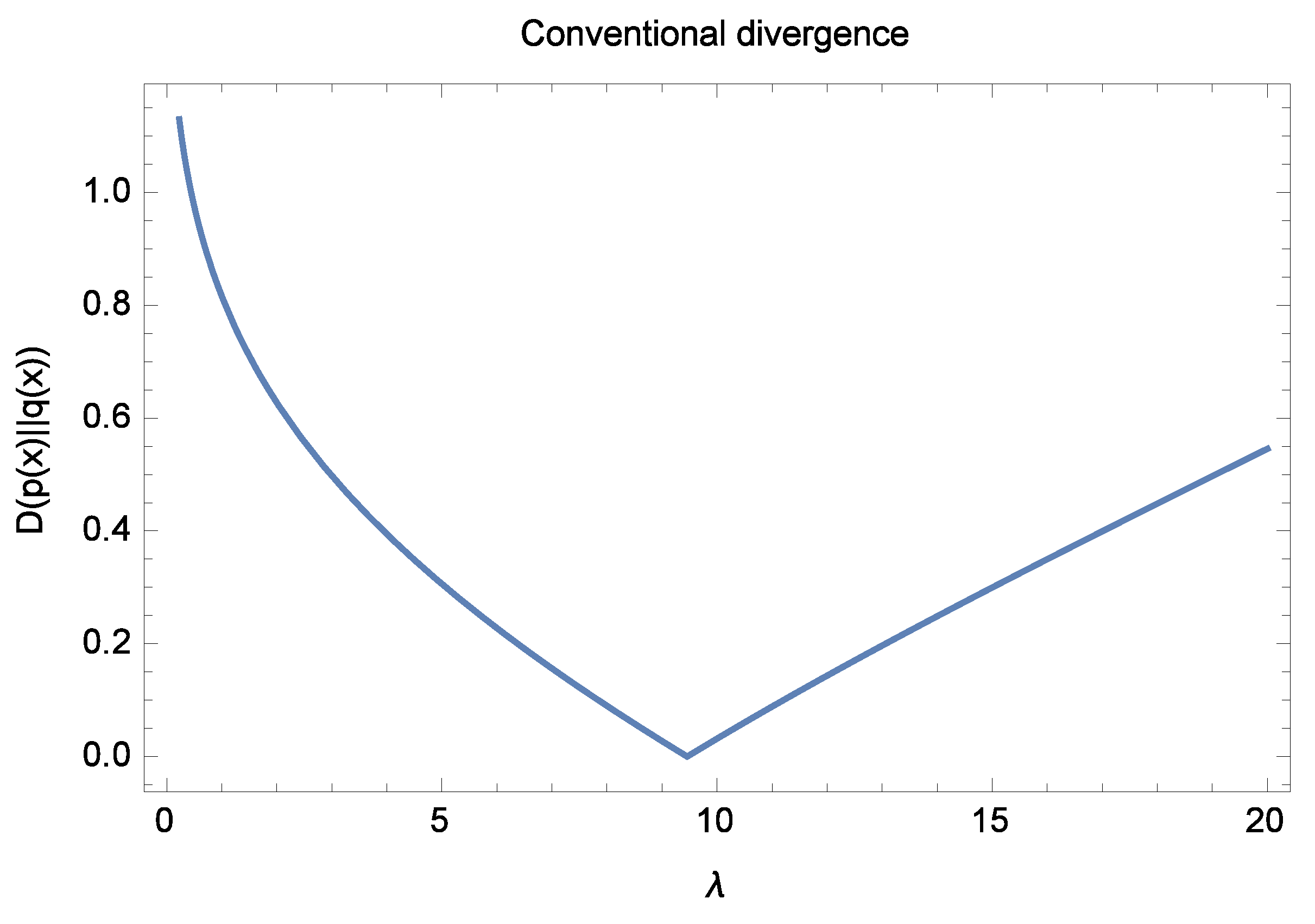
Figure 2.
For , the (a) conventional and (b) fractional divergence is shown, respectively.
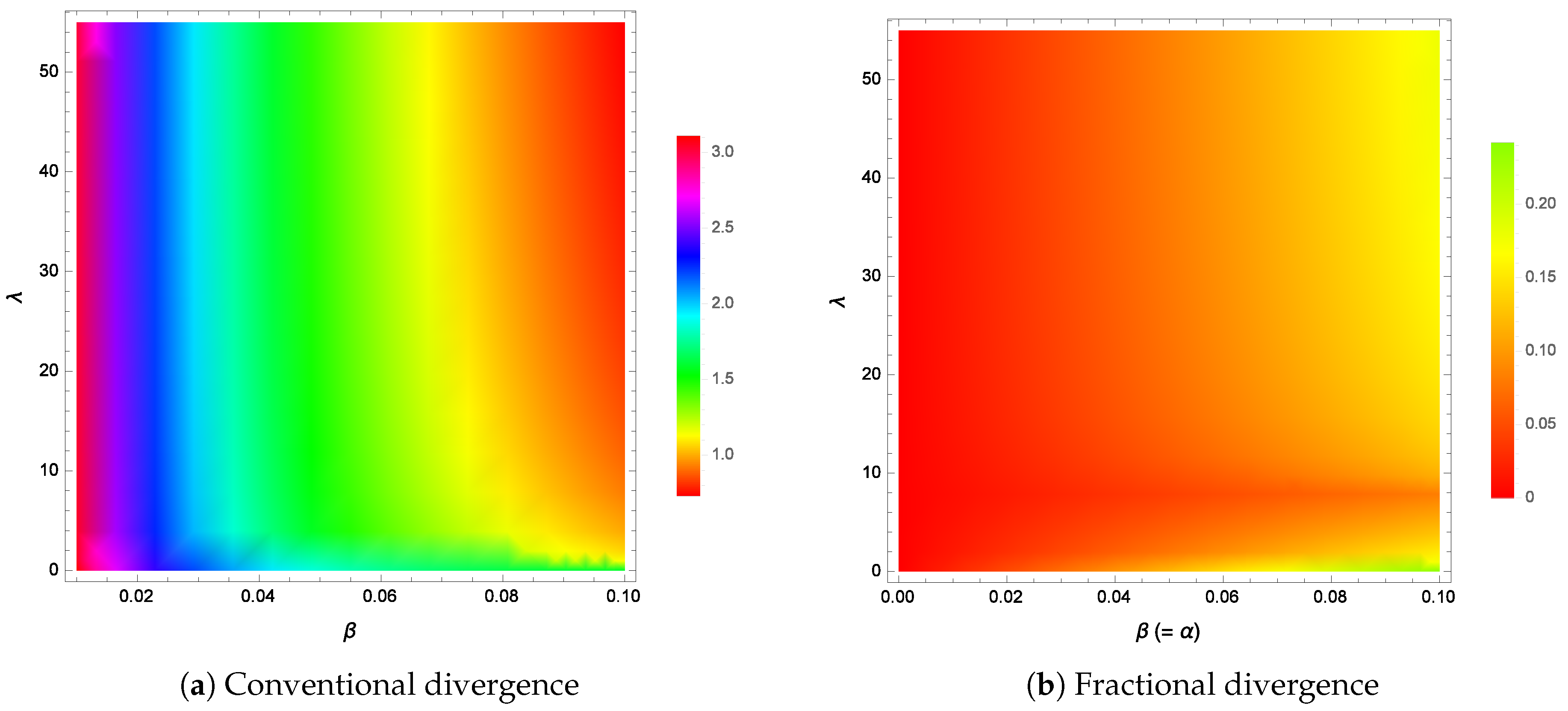
Figure 3.
Variation of the (fractional) divergence manifold between two Exponential-densities in terms of the fractional orders and . The case corresponds to the conventional divergence.
Figure 3.
Variation of the (fractional) divergence manifold between two Exponential-densities in terms of the fractional orders and . The case corresponds to the conventional divergence.
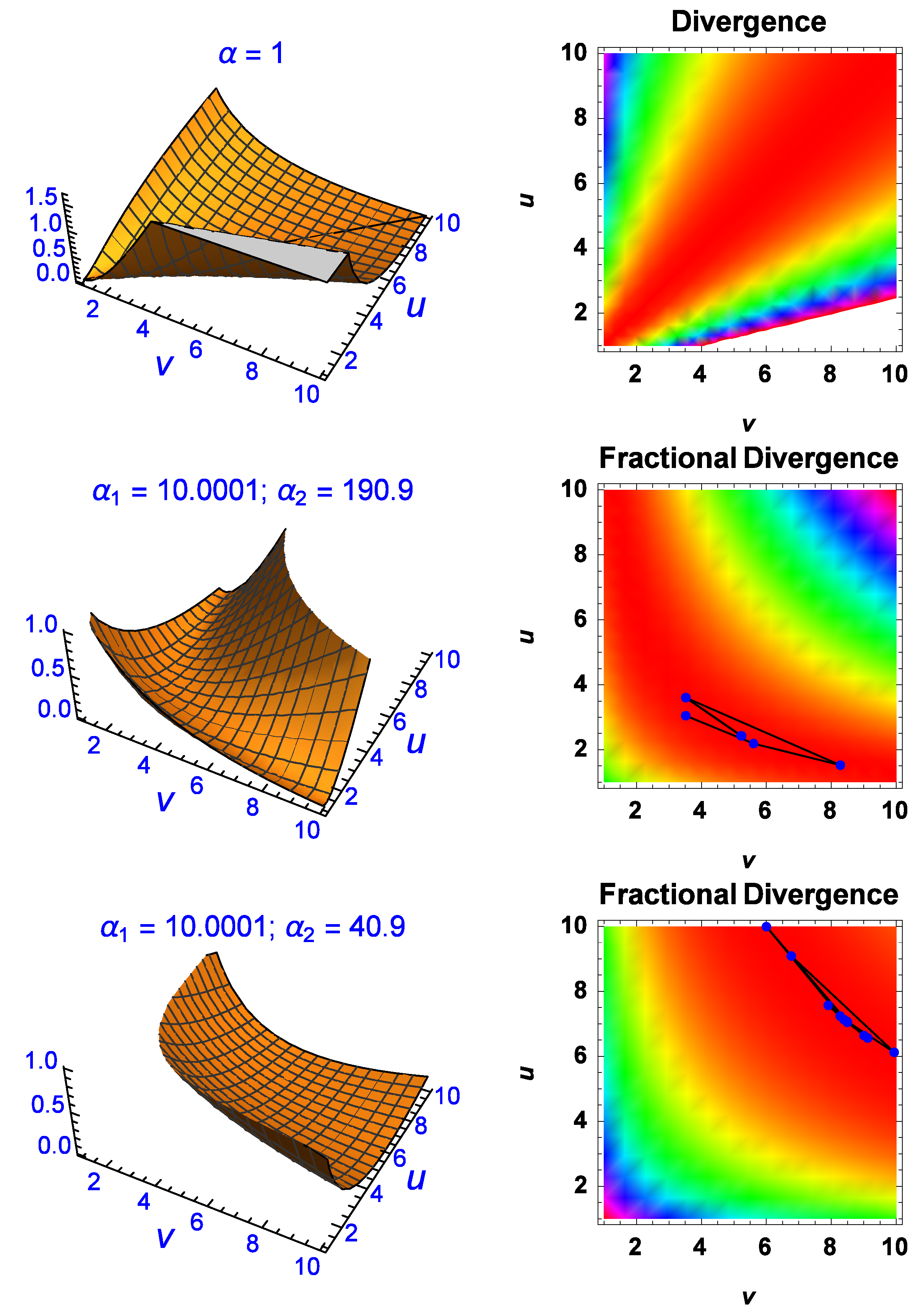
Figure 4.
Further manipulation of the (fractional) divergence manifold between two Exponential-densities via the fractional orders and .
Figure 4.
Further manipulation of the (fractional) divergence manifold between two Exponential-densities via the fractional orders and .
© 2017 by the author. Licensee MDPI, Basel, Switzerland. This article is an open access article distributed under the terms and conditions of the Creative Commons Attribution (CC BY) license (http://creativecommons.org/licenses/by/4.0/).
Share and Cite
MDPI and ACS Style
Alexopoulos, A. Fractional Divergence of Probability Densities. Fractal Fract. 2017, 1, 8. https://doi.org/10.3390/fractalfract1010008
AMA Style
Alexopoulos A. Fractional Divergence of Probability Densities. Fractal and Fractional. 2017; 1(1):8. https://doi.org/10.3390/fractalfract1010008
Chicago/Turabian StyleAlexopoulos, Aris. 2017. "Fractional Divergence of Probability Densities" Fractal and Fractional 1, no. 1: 8. https://doi.org/10.3390/fractalfract1010008