Fractional Velocity as a Tool for the Study of Non-Linear Problems

Abstract

Singular functions and, in general, Hölder functions represent conceptual models of nonlinear physical phenomena. The purpose of this survey is to demonstrate the applicability of fractional velocities as tools to characterize Hölder and singular functions, in particular. Fractional velocities are defined as limits of the difference quotients of a fractional power and they generalize the local notion of a derivative. On the other hand, their properties contrast some of the usual properties of derivatives. One of the most peculiar properties of these operators is that the set of their non trivial values is disconnected. This can be used for example to model instantaneous interactions, for example Langevin dynamics. Examples are given by the De Rham and Neidinger’s singular functions, represented by limits of iterative function systems. Finally, the conditions for equivalence with the Kolwankar-Gangal local fractional derivative are investigated.

1. Introduction

Non-linear and fractal physical phenomena are abundant in nature [1,2]. Examples of non-linear phenomena can be given by the continuous time random walks resulting in fractional diffusion equations [3], fractional conservation of mass [4] or non-linear viscoelasticity [5,6]. Such models exhibit global dependence through the action of the nonlinear convolution operator (i.e., differ-integral). Since this setting opposes the principle of locality there can be problems with the interpretation of the obtained results. In most circumstances such models can be treated as asymptotic as it has been demonstrated for the time-fractional continuous time random walk [7]. The asymptotic character of these models leads to the realization that they describe mesoscopic behavior of the concerned systems. The action of fractional differ-integrals on analytic functions results in Hölder functions representable by fractional power series (see for example [8]).

Fractals are becoming essential components in the modeling and simulation of natural phenomena encompassing many temporal or spatial scales [9]. The irregularity and self-similarity under scale changes are the main attributes of the morphologic complexity of cells and tissues [10]. Fractal shapes are frequently built by iteration of function systems via recursion [11,12]. In a large number of cases, these systems leads to nowhere differentiable fractals of infinite length, which may be unrealistic. On the other hand fractal shapes observable in natural systems typically span only several recursion levels. This fact draws attention to one particular class of functions, called singular, which are differentiable but for which at most points the derivative vanishes. There are fewer tools for the study of singular functions since one of the difficulties is that for them the Fundamental Theorem of calculus fails and hence they cannot be represented by a non-trivial differential equation.

Singular signals can be considered as toy-models for strongly-non linear phenomena, such as turbulence or asset price dynamics. In the beginning of 1970s, Mandelbrot proposed a model of random energy dissipation in intermittent turbulence [13], which served as one of the early examples of multifractal formalism. This model, known as canonical Mandelbrot cascades, is related to the Richardson’s model of turbulence as noted in [14,15]. Mandelbrot’s cascade model and its variations try to mimic the way in which energy is dissipated, i.e., the splitting of eddies and the transfer of energy from large to small scales. There is an interesting link between multifractals and Brownian motion [16]. One of the examples in the present paper can be related to the Mandelbrot model and the associated binomial measure.

Mathematical descriptions of strongly non-linear phenomena necessitate relaxation of the assumption of differentiability [17]. While this can be achieved also by fractional differ-integrals, or by multi-scale approaches [18], the present work focuses on local descriptions in terms of limits of difference quotients [19] and non-linear scale-space transformations [20]. The reason for this choice is that locality provides a direct way of physical interpretation of the obtained results. In the old literature, difference quotients of functions of fractional order have been considered at first by du Bois-Reymond [21] and Faber [22] in their studies of the point-wise differentiability of functions. While these initial developments followed from purely mathematical interest, later works were inspired from physical research questions. Cherbit [19] and later on Ben Adda and Cresson [23] introduced the notion of fractional velocity as the limit of the fractional difference quotient. Their main application was the study of fractal phenomena and physical processes for which the instantaneous velocity was not well defined [19].

This work will further demonstrate applications to singular functions. Examples are given by the De Rham and Neidinger’s functions, represented by iterative function systems (IFS). The relationship with the Mandelbrot cascade and the associated Bernoulli-Mandelbrot binomial measure is also put into evidence. In addition, the form of the Langevin equation is examined for the requirements of path continuity. Finally, the relationship between fractional velocities and the localized versions of fractional derivatives in the sense of Kolwankar-Gangal will be demonstrated.

2. Fractional Variations and Fractional Velocities

The general definitions and notations are given in Appendix A. This section introduces the concept of fractional variation and fractional velocities.

Definition 1.

Define forward (backward) Fractional Variation operators of order $0\le \beta \le 1$ as

$$\begin{array}{c}\hfill {\upsilon }_{ϵ\pm }^{\beta }\left[f\right]\left(x\right):=\frac{{\Delta }_{ϵ}^{\pm }\left[f\right]\left(x\right)}{{ϵ}^{\beta }}\end{array}$$

(1)

for a positive ϵ.

Definition 2

(Fractional order velocity). Define the fractional velocity of fractional order β as the limit

$$\begin{array}{cc}\hfill {\upsilon }_{\pm }^{\beta }f\left(x\right)& :=\underset{ϵ\to 0}{\lim }\frac{{\Delta }_{ϵ}^{\pm }\left[f\right]\left(x\right)}{{ϵ}^{\beta }}=\underset{ϵ\to 0}{\lim }{\upsilon }_{ϵ\pm }^{\beta }\left[f\right]\left(x\right).\hfill \end{array}$$

(2)

A function for which at least one of ${\upsilon }_{\pm }^{\beta }f\left(x\right)$ exists finitely will be called β-differentiable at the point x.

The terms $\beta$-velocity and fractional velocity will be used interchangeably throughout the paper. In the above definition we do not require upfront equality of left and right $\beta$-velocities. This amounts to not demanding continuity of the $\beta$-velocities in advance. Instead, continuity is a property, which is fulfilled under certain conditions. It was further established that for fractional orders fractional velocity is continuous only if it is zero [24].

Further, the following technical conditions are important for applications.

Condition 1

(Hölder growth condition). For given x and $0<\beta \le 1$

$${\mathrm{osc}}_{ϵ}^{\pm }f\left(x\right)\le C{ϵ}^{\beta }$$

(C1)

for some $C\ge 0$ and $ϵ>0$.

Condition 2

(Hölder oscillation condition). For given x, $0<\beta \le 1$ and $ϵ>0$

$${\mathrm{osc}}^{\pm }{\upsilon }_{ϵ\pm }^{\beta }\left[f\right]\left(x\right)=0.$$

(C2)

The conditions for the existence of the fractional velocity were demonstrated in [24]. The main result is repeated here for convenience.

Theorem 1

(Conditions for existence of β-velocity). For each $\beta >0$ if ${\upsilon }_{+}^{\beta }f\left(x\right)$ exists (finitely), then f is right-Hölder continuous of order β at x and C1 holds, and the analogous result holds for ${\upsilon }_{-}^{\beta }f\left(x\right)$ and left-Hölder continuity.

Conversely, if C2 holds then ${\upsilon }_{\pm }^{\beta }f\left(x\right)$ exists finitely. Moreover, C2 implies C1.

The proof is given in [24]. The essential algebraic properties of the fractional velocity are given in Appendix B. Fractional velocities provide a local way of approximating the growth of Hölder functions in the following way.

Proposition 1

(Fractional Taylor-Lagrange property). The existence of ${\upsilon }_{\pm }^{\beta }f\left(x\right)\ne 0$ for $\beta \le 1$ implies that

$$f(x\pm ϵ)=f\left(x\right)\pm {\upsilon }_{\pm }^{\beta }f\left(x\right){ϵ}^{\beta }+\mathcal{O}\left({ϵ}^{\beta }\right).$$

(3)

While if

$$f(x\pm ϵ)=f\left(x\right)\pm K{ϵ}^{\beta }+{\gamma }_{ϵ}{ϵ}^{\beta }$$

uniformly in the interval $x\in [x,x+ϵ]$ for some Cauchy sequence ${\gamma }_{ϵ}=\mathcal{O}\left(1\right)$ and $K\ne 0$ is constant in ϵ then ${\upsilon }_{\pm }^{\beta }f\left(x\right)$ = K.

The proof is given in [24].

Remark 1.

The fractional Taylor-Lagrange property was assumed and applied to establish a fractional conservation of mass formula in ([4], Section 4) assuming the existence of a fractional Taylor expansion according to Odibat and Shawagfeh [25]. These authors derived fractional Taylor series development using repeated application of Caputo’s fractional derivative [25].

The Hölder growth property can be generalized further into the concept of F-analytic functions (see Appendix A for definition). An F-analytic function can be characterized up to the leading fractional order in terms of its $\alpha$-differentiability.

Proposition 2.

Suppose that $f\in {\mathbb{F}}^E$ in the interval $I=[x,x+ϵ]$. Then ${\upsilon }_{\pm }^{\alpha }f\left(x\right)$ exists finitely for $\alpha \in [0,min\mathbb{E}]$.

Proof. 

The proof follows directly from Proposition 1 observing that

$$\sum _{{\alpha }_j\in E\setminus \left\{{\alpha }_1\right\}}{a}_j(x-b_j)=\mathcal{O}\left(|x-b_j{|}^{{\alpha }_1}\right)$$

so that using the notation in Definition A4

$${\upsilon }_{+}^{{\alpha }_1}f\left(x\right)=a_1,{\upsilon }_{-}^{{\alpha }_1}f\left(x\right)=0$$

 ☐

Remark 2.

From the proof of the proposition one can also see the fundamental asymmetry between the forward and backward fractional velocities. A way to combine this is to define a complex mapping

$${\upsilon }_C^{\beta }f\left(x\right):={\upsilon }_{+}^{\beta }f\left(x\right)+{\upsilon }_{-}^{\beta }f\left(x\right)\pm i\left({\upsilon }_{+}^{\beta }f\left(x\right)-{\upsilon }_{-}^{\beta }f\left(x\right)\right)$$

which is related to the approach taken by Nottale [17] by using complexified velocity operators. However, such unified treatment will not be pursued in this work.

3. Characterization of Singular Functions

3.1. Scale Embedding of Fractional Velocities

As demonstrated previously, the fractional velocity has only “few” non-zero values [24,26]. Therefore, it is useful to discriminate the set of arguments where the fractional velocity does not vanish.

Definition 3.

The set of points where the fractional velocity exists finitely and ${\upsilon }_{\pm }^{\beta }f\left(x\right)\ne 0$ will be denoted as the set of change ${\chi }_{\pm }^{\beta }\left(f\right):=\left\{x:{\upsilon }_{\pm }^{\beta }f\left(x\right)\ne 0\right\}$.

Since the set of change ${\chi }_{+}^{\alpha }\left(f\right)$ is totally disconnected [24] some of the useful properties of ordinary derivatives, notably the continuity and the semi-group composition property, are lost. Therefore, if we wish to retain the continuity of description we need to pursue a different approach, which should be equivalent in limit. Moreover, we can treat the fractional order of differentiability (which coincides with the point-wise Hölder exponent, that is Condition C1) as a parameter to be determined from the functional expression.

One can define two types of scale-dependent operators for a wide variety if physical signals. An extreme case of such signals are the singular functions

Since for a singular signal the derivative either vanishes or it diverges then the rate of change for such signals cannot be characterized in terms of derivatives. One could apply to such signals either the fractal variation operators of certain order or the difference quotients as Nottale does and avoid taking the limit. Alternately, as will be demonstrated further, the scale embedding approach can be used to reach the same goal.

Singular functions can arise as point-wise limits of continuously differentiable ones. Since the fractional velocity of a continuously-differentiable function vanishes we are lead to postpone taking the limit and only apply L’Hôpital’s rule, which under the hypotheses detailed further will reach the same limit as $ϵ\to 0$. Therefore, we are set to introduce another pair of operators which in limit are equivalent to the fractional velocities notably these are the left (resp. right) scale velocity operators:

$$\begin{array}{c}\hfill {\mathcal{S}}_{ϵ\pm }^{\beta }\left[f\right]\left(x\right):=\frac{{ϵ}^{\beta }}{{\left\{\beta \right\}}_1}\frac{\partial }{\partial ϵ}f(x\pm ϵ)\end{array}$$

(6)

where ${\left\{\beta \right\}}_1\equiv 1-\beta \mathrm{mod}1$. The $ϵ$ parameter, which is not necessarily small, represents the scale of observation.

The equivalence in limit is guaranteed by the following result:

Proposition 3.

Let $f^{\prime }\left(x\right)$ be continuous and non-vanishing in $I=(x,x\pm \mu )$. That is $f\in AC\left[I\right]$. Then

$$\underset{ϵ\to 0}{\lim }{\upsilon }_{ϵ\pm }^{1-\beta }\left[f\right]\left(x\right)=\underset{ϵ\to 0}{\lim }{\mathcal{S}}_{ϵ\pm }^{\beta }\left[f\right]\left(x\right)$$

if one of the limits exits.

The proof is given in [20] and will not be repeated. In this formulation the value of $1-\beta$ can be considered as the magnitude of deviation from linearity (or differentiability) of the signal at that point.

Theorem 2

(Scale velocity fixed point). Suppose that $f\in BVC[x,x+ϵ]$ and $f^{\prime }$ does not vanish a.e. in $[x,x+ϵ]$. Suppose that $\varphi \in {\mathbb{C}}^1$ is a contraction map. Let $f_n\left(x\right):={\underbrace{\varphi \circ \dots \varphi }}_n\circ f\left(x\right)$ be the n-fold composition and $F\left(x\right):=\underset{n\to \infty }{\lim }{f}_n\left(x\right)$ exists finitely. Then the following commuting diagram holds:

The limit in n is taken point-wise.

Proof. 

The proof follows by induction. Only the forward case will be proven. The backward case follows by reflection of the function argument. Consider an arbitrary n and an interval $I=[x,x+ϵ]$. By differentiability of the map $\varphi$

$${\upsilon }_{+}^{\beta }{f}_n\left(x\right)={\left(\frac{\partial \varphi }{\partial f}\right)}^n{\upsilon }_{+}^{\beta }f\left(x\right)$$

Then by hypothesis $f^{\prime }\left(x\right)$ exists finitely a.e. in I so that

$${\upsilon }_{+}^{\beta }f\left(x\right)=\frac{1}{\beta }\underset{ϵ\to 0}{\lim }{ϵ}^{1-\beta }{f}^{\prime }(x+ϵ)$$

so that

$${\upsilon }_{+}^{\beta }{f}_n\left(x\right)=\frac{1}{\beta }{\left(\frac{\partial \varphi }{\partial f}\right)}^n\underset{ϵ\to 0}{\lim }{ϵ}^{1-\beta }{f}^{\prime }(x+ϵ)$$

On the other hand

$${\mathcal{S}}_{ϵ+}^{1-\beta }\left[f_n\right]\left(x\right)=\frac{1}{\beta }{\left(\frac{\partial \varphi }{\partial f}\right)}^n{ϵ}^{1-\beta }{f}^{\prime }(x+ϵ)$$

Therefore, if the RHS limits exist they are the same. Therefore, the equality is asserted for all n.

Suppose that ${\upsilon }_{+}^{\beta }F\left(x\right)$ exists finitely.

Since $\varphi$ is a contraction and $F\left(x\right)$ is its fixed point then by Banach fixed point theorem there is a Lipschitz constant $q<1$ such that

$$\begin{array}{cc}\hfill \underset{A}{\underbrace{|F(x+ϵ)-f_n(x+ϵ)|}}& \le \frac{q^n}{1-q}|\varphi \circ f(x+ϵ)-f(x+ϵ)|\hfill \\ \hfill \underset{B}{\underbrace{|F\left(x\right)-f_n\left(x\right)|}}& \le \frac{q^n}{1-q}|\varphi \circ f\left(x\right)-f\left(x\right)|\hfill \end{array}$$

Then by the triangle inequality

$$|{\Delta }_{ϵ}^{+}\left[F\right]\left(x\right)-{\Delta }_{ϵ}^{+}\left[f_n\right]\left(x\right)|\le A+B\le \frac{q^n}{1-q}\left(|\varphi \circ f(x+ϵ)-f(x+ϵ)|+|\varphi \circ f(x)-f(x)|\right)\le q^{n}L$$

for some L. Then

$$|{\upsilon }_{ϵ+}^{\beta }\left[F\right]\left(x\right)-{\upsilon }_{ϵ+}^{\beta }\left[f_n\right]\left(x\right)|\le \frac{q^{n}L}{{ϵ}^{\beta }}$$

We evaluate $ϵ=q^n/\lambda$ for some $\lambda \ge 1$ so that

$$|{\upsilon }_{ϵ+}^{\beta }\left[F\right]\left(x\right)-{\upsilon }_{ϵ+}^{\beta }\left[f_n\right]\left(x\right)|\le q^{n(1-\beta )}L{\lambda }^{\beta }=:{\mu }_n$$

Therefore, in limit RHS $\underset{n\to \infty }{\lim }{\mu }_n=0$. Therefore,

$$\underset{n\to \infty }{\lim }{\upsilon }_{ϵ+}^{\beta }\left[f_n\right]\left(x\right)={\upsilon }_{+}^{\beta }F\left(x\right)|{ϵ}_n\to 0$$

Therefore, by continuity of ${\mu }_n$ in the $\lambda$ variable the claim follows. ☐

So stated, the theorem holds also for sets of maps ${\varphi }_k$ acting in sequence as they can be identified with an action of a single map.

Corollary 1.

Let $\mathsf{\Phi }=\left\{{\varphi }_k\right\}$, where the domains of ${\varphi }_k$ are disjoint and the hypotheses of Theorem 2 hold. Then Theorem 2 holds for Φ.

Corollary 2.

Under the hypotheses of Theorem 2 for $f\in {\mathbb{H}}^{\alpha }$ and $\frac{\partial \varphi }{\partial f}>1$ there is a Cauchy null sequence ${\left\{ϵ\right\}}_k^{\infty }$, such that

$$\underset{n\to \infty }{\lim }{\mathcal{S}}_{{ϵ}_n\pm }^{1-\alpha }{f}_n\left(x\right)={\upsilon }_{\pm }^{\alpha }f\left(x\right)$$

This sequence will be named scale–regularizing sequence.

Proof. 

In the proof of the theorem it was established that

$${\mathcal{S}}_{ϵ+}^{1-\alpha }\left[f_n\right]\left(x\right)=\frac{1}{\beta }{\left(\frac{\partial \varphi }{\partial f}\right)}^n{ϵ}^{1-\alpha }{f}^{\prime }(x+ϵ)$$

Then we can identify

$${ϵ}_n=\pm ϵ/{\left|\frac{\partial \varphi }{\partial f}\right|}^{n/(1-\alpha )}$$

for some $ϵ<1$ so that

$${\mathcal{S}}_{ϵ+}^{1-\alpha }\left[f_n\right]\left(x\right)={\mathcal{S}}_{{ϵ}_n}^{1-\alpha }\left[f\right]\left(x\right)$$

Then since $\frac{\partial \varphi }{\partial f}>1$ we have ${ϵ}_{n+1}<{ϵ}_n<1$. Therefore, ${\left\{{ϵ}_k\right\}}_k$ is a Cauchy sequence. Further, the RHS limit evaluates to (omitting n for simplicity)

$$\underset{ϵ\to 0}{\lim }{\mathcal{S}}_{ϵ\pm }^{1-\alpha }\left[f\right]\left(x\right)=\frac{1}{\alpha }\underset{ϵ\to 0}{\lim }{ϵ}^{1-\alpha }{f}^{\prime }(x\pm ϵ)={\upsilon }_{\pm }^{\alpha }f\left(x\right)$$

The backward case can be proven by identical reasoning. ☐

Therefore, we can identify the Lipschitz constant q by the properties of the contraction maps as will be demonstrated in the following examples.

3.2. Applications

3.2.1. De Rham Function

De Rham’s function arises in several applications. Lomnicki and Ulan [27] have given a probabilistic construction. In a an imaginary experiment of flipping a possibly “unfair” coin with probability a of heads (and $1-a$ of tails). Then $R_a\left(x\right)=\mathbb{P}\left\{t\le x\right\}$ after infinitely many trials where t is the record of the trials.

Mandelbrot [13] introduces a multiplicative cascade, describing energy dissipation in turbulance, which is related to the increments of the De Rham’s function.

The function can be defined in different ways [22,28,29]. One way to define the De Rham’s function is as the unique solutions of the functional equations

$$R_a\left(x\right):=\left\{\begin{array}{cc}a{R}_a\left(2x\right),\hfill & 0\le x<\frac{1}{2}\hfill \\ (1-a)R_a(2x-1)+a,\hfill & \frac{1}{2}\le x\le 1\hfill \end{array}\right.$$

and boundary values $R_a\left(0\right)=0$, $R_a\left(1\right)=1$. The function is strictly increasing and singular. Its scaling properties and additional functional equations are described in [30].

In another re-parametrization the defining functional equations become

$$\begin{array}{cc}\hfill R_a\left(x\right)& =a{R}_a\left(2x\right)\hfill \\ \hfill R_a(x+1/2)& =(1-a)R_a\left(2x\right)+a\hfill \end{array}$$

In addition, there is a symmetry with respect to inversion about 1.

$$R_a\left(x\right)=1-R_{1-a}(1-x)$$

De Rham’s function is also known under several different names—“Lebesgue’s singular function” or “Salem’s singular function”.

De Rham’s function can be re-parametrized on the basis of the point-wise Hölder exponent [20]. Then it is the fixed point of the following IFS:

$$r_n(x,\alpha ):=\left\{\begin{array}{cc}{x}^{\alpha },\hfill & n=0\hfill \\ \frac{1}{2^{\alpha }}{r}_{n-1}(2x,\alpha ),\hfill & 0\le x<\frac{1}{2}\hfill \\ (1-\frac{1}{2^{\alpha }})r_{n-1}(2x-1,\alpha )+\frac{1}{2^{\alpha }},\hfill & \frac{1}{2}\le x\le 1\hfill \end{array}\right.$$

provided that $a=1/2^{\alpha },a\ge 1/2$. For the case $a\le 1/2$ the parametrization corresponding to the original IFS is $\alpha =-{log}_2(1-a)$. The IFS converges point-wise to $R_{\alpha }\left(x\right)=\underset{n\to \infty }{\lim }{r}_n(x,\alpha )$.

Formal calculation shows that

$${\upsilon }_{+}^{\beta }{r}_n(x,\alpha ):=\left\{\begin{array}{cc}{2}^{\beta -\alpha }{\upsilon }_{+}^{\beta }{r}_{n-1}(2x,\alpha ),\hfill & 0\le x<\frac{1}{2}\hfill \\ (2^{\alpha }-1)2^{\beta -\alpha }{\upsilon }_{+}^{\beta }{r}_{n-1}(2x-1,\alpha ),\hfill & \frac{1}{2}\le x\le 1\hfill \end{array}\right.$$

Therefore, for $\beta <\alpha$ the fractional velocity vanishes, while for $\beta >\alpha$ it diverges. We further demonstrate its existence for $\beta =\alpha$. For this case formally

$${\upsilon }_{+}^{\alpha }{r}_n(x,\alpha ):=\left\{\begin{array}{cc}{\upsilon }_{+}^{\alpha }{r}_{n-1}(2x,\alpha ),\hfill & 0\le x<\frac{1}{2}\hfill \\ (2^{\alpha }-1){\upsilon }_{+}^{\alpha }{r}_{n-1}(2x-1,\alpha ),\hfill & \frac{1}{2}\le x\le 1\hfill \end{array}\right.$$

and ${\upsilon }_{+}^a{r}_0(x,\alpha )=\mathbf{1}(x=0)$.

The same result can be reached using scaling arguments. We can discern two cases.

Case 1, $x\le 1/2$ : Then application of the scale operator leads to :

$${\mathcal{S}}_{ϵ+}^{1-\alpha }\left[r_n\right]\left(x,\alpha \right)=\frac{2^{1-\alpha }{ϵ}^{1-\alpha }}{\alpha }\frac{\partial }{\partial ϵ}{r}_{n-1}(2x+2ϵ,\alpha )$$

Therefore, the pre-factor will remain scale invariant for $ϵ=1/2$ and consecutively ${ϵ}_n=\frac{1}{2^n}$ so that we identify a scale-regularizing Cauchy sequence so that $f\left(x\right)=x^a$ is verified and ${\upsilon }_{+}^{\alpha }{R}_a\left(0\right)=1$.

Case 2, $x>1/2$: In a similar way :

$${\mathcal{S}}_{ϵ+}^{1-\alpha }\left[r_n\right]\left(x,\alpha \right)=\frac{2^{1-\alpha }{ϵ}^{1-\alpha }}{\alpha }\left(2^{\alpha }-1\right)\frac{\partial }{\partial ϵ}{r}_{n-1}(2x+2ϵ-1,\alpha )$$

Applying the same sequence results in a factor $2^a-1\le 1$. Therefore, the resulting transformation is a contraction.

Finally, we observe that if $x=\overline{0.d_1\dots d_n}$ is in binary representation then the number of occurrences of Case 2 corresponds to the number of occurrences of the digit 1 in the binary notation (see below).

The calculation can be summarized in the following proposition:

Proposition 4.

Let ${\mathbb{Q}}_2$ denote the set of dyadic rationals. Let $s_n={\displaystyle \sum _{k=1}^n}{d}_k$ denote the sum of the digits for the number $x=\overline{0.d_1\dots d_n},d\in \{0,1\}$ in binary representation, then

$${\upsilon }_{+}^{\alpha }{R}_a\left(x\right)=\left\{\begin{array}{cc}{\left(2^{\beta }-1\right)}^{s_n},\hfill & x\in {\mathbb{Q}}_2\hfill \\ 0,\hfill & x\notin {\mathbb{Q}}_2\hfill \end{array}\right.$$

for $\alpha =-lo{g}_{2}a$, $a>\frac{1}{2}$. For $\alpha <-lo{g}_{2}a$ ${\upsilon }_{+}^{\alpha }{R}_a\left(x\right)=0$.

3.2.2. Bernoulli-Mandelbrot Binomial Measure

The binomial Mandlebrot measure $m_a$ is constructed as follows. Let ${\mathcal{T}}_n$ be the complete partition of dyadic intervals of the n-th generation on ${\mathcal{T}}_0:=[0,1)$. In addition, let’s assume the generative scheme

$${\mathcal{T}}_n\mapsto ({\mathcal{T}}_{n+1}^L,{\mathcal{T}}_{n+1}^R)$$

where the interval ${\mathcal{T}}_n=\left[x_n,x_n+\frac{1}{2^n}\right)$ is split into a left and right children such that

$${\mathcal{T}}_{n+1}^L\bigcup {\mathcal{T}}_{n+1}^R={\mathcal{T}}_n,{\mathcal{T}}_{n+1}^L\bigcap {\mathcal{T}}_{n+1}^R=\varnothing .$$

Let

$${\mathcal{T}}_{n+1}^L=\left[x_n^L,x_{n+1}^L+\frac{1}{2^{n+1}}\right),{\mathcal{T}}_{n+1}^R=\left[x_n^R,x_{n+1}^R+\frac{1}{2^{n+1}}\right).$$

Then define the measure $m_a$ recursively as follows:

$$\begin{array}{cc}\hfill m_a\left({\mathcal{T}}_{n+1}^L\right)& =a{m}_a\left({\mathcal{T}}_n\right),\hfill \\ \hfill m_a\left({\mathcal{T}}_{n+1}^R\right)& =(1-a)m_a\left({\mathcal{T}}_n\right),\hfill \\ \hfill m_a\left({\mathcal{T}}_0\right)& =1.\hfill \end{array}$$

The construction is presented in the diagram below:

Therefore,

$$x_{n+1}^L+\frac{1}{2^{n+1}}=x_{n+1}^R$$

so that all $x_n\in {\mathbb{Q}}_2^{}$.

To elucidate the link to the Mandlebrot measure we turn to the arithmetic representation of the De Rham function. That is, consider $x=\overline{0.d_1\dots d_n},d\in \{0,1\}$ under the convention that for a dyadic rational the representation terminates. Then according to Lomnicki and Ulam [27]

$$\begin{array}{cc}\hfill R_a\left(x\right)& =\sum _{k=1}^n{d}_k{a}^{k-s_n+1}{(1-a)}^{s_n-1},s_n=\sum _{k=1}^n{d}_k\hfill \end{array}$$

Consider the increment of $R_a\left(x\right)$ for $ϵ=1/2^{n+1}$. If $x=\overline{0.d_1\dots d_n}$ then $x+1/2^{n+1}=\overline{0.d_1\dots d_{n}1}$ so that

$$D\left(x\right):=R_a\left(x+1/2^{n+1}\right)-R_a\left(x\right)=a^{n+1-s_n}{(1-a)}^{s_n}=a^{n+1}{\left(1/a-1\right)}^{s_n}.$$

From this it is apparent that

$$D\left(x\right)=aD\left(2x\right),x<1/2D\left(x\right)=(1-a)D(2x-1),x\ge 1/2$$

Therefore, we can identify $D\left(x\right)=m_a\left(\mathcal{T}\right)$ for $x\in \mathcal{T}$.

On the other hand, for $a=1/2^{\alpha }$

$${\upsilon }_{ϵ+}^{\alpha }\left[R_a\right]\left(x\right)=\frac{D\left(x\right)}{1/2^{(n+1)\alpha }}=2^{(n+1)\alpha }{m}_a\left({\mathcal{T}}_{n+1}\right)$$

for $x\in {\mathcal{T}}_{n+1}$.

Remark 3.

It should be noted that based on the symmetry equation

$${\upsilon }_{+}^{\alpha }{R}_a\left(x\right)={\upsilon }_{-}^{\alpha }{R}_a\left(1-x\right)$$

so that ${\upsilon }_{+}^{\alpha }{R}_a\left(x\right)\ne {\upsilon }_{-}^{\alpha }{R}_a\left(x\right)$ for $\alpha \ne 1$ so that the measure $m_a$ does not have a density in agreement with Marstrand’s theorem.

3.2.3. Neidinger Function

Neidinger introduces a novel strictly singular function [31], which he called fair-bold gambling function. The function is based on De Rham’s construction. The Neidinger’s function is defined as the limit of the system

$$N_n(x,a):=\left\{\begin{array}{cc}x,\hfill & n=0\hfill \\ a\leftarrow 1-a\hfill & \\ a{N}_{n-1}(2x,1-a),\hfill & 0\le x<\frac{1}{2}\hfill \\ (1-a)N_{n-1}(2x-1,1-a)+a,\hfill & \frac{1}{2}\le x\le 1\hfill \end{array}\right.$$

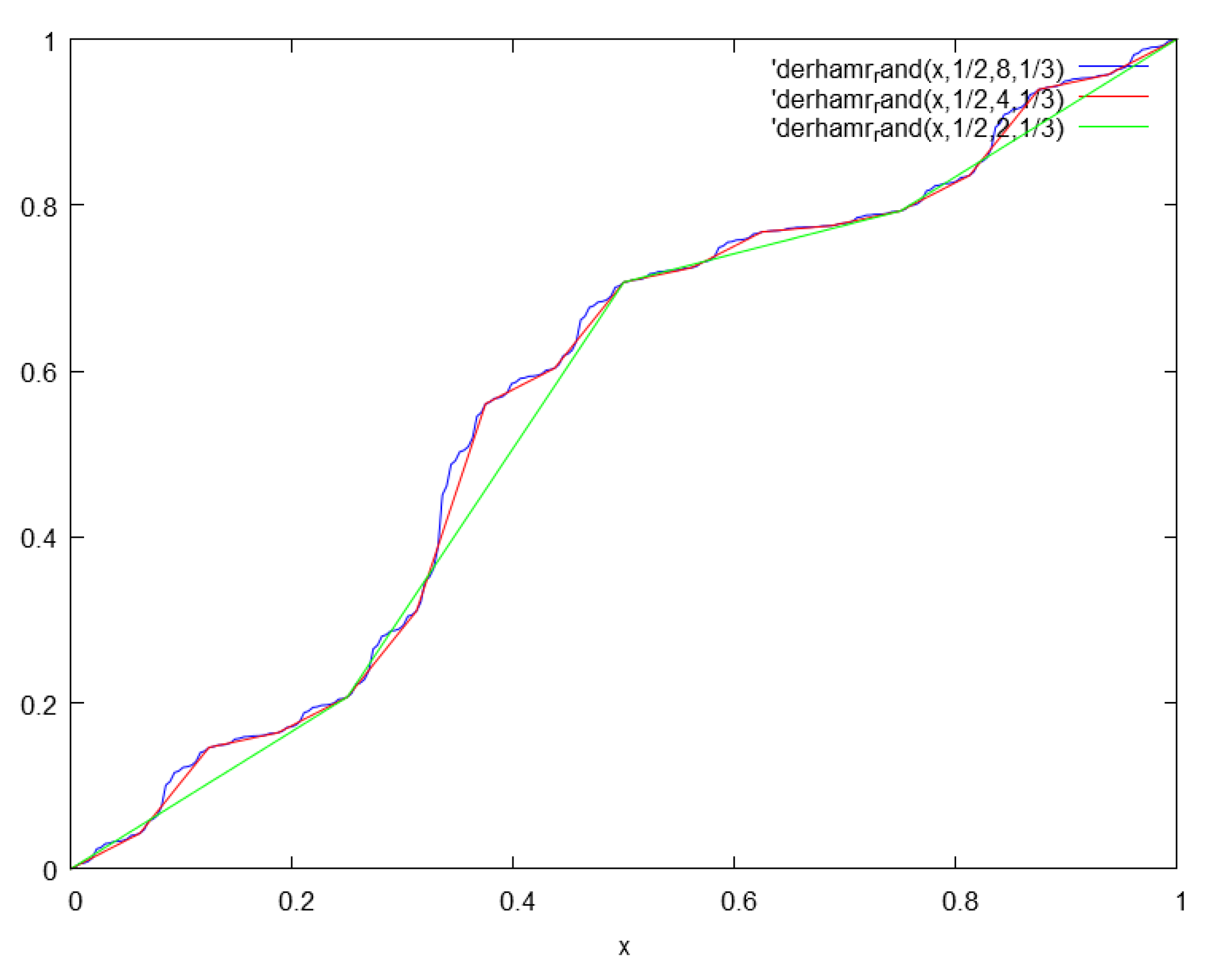
In other words the parameter a alternates for every recursion step but is not passed on the next function call (see Figure 1).

We can exercise a similar calculation again starting from $r_0(x,a)=x^a$. Then

$${\upsilon }_{+}^{\beta }{r}_n(x,a):=\left\{\begin{array}{cc}a\leftarrow 1-a,\hfill & neven\hfill \\ a{2}^{\beta }{\upsilon }_{+}^{\beta }{r}_{n-1}(2x,a),\hfill & 0\le x<\frac{1}{2}\hfill \\ (1-a)2^{\beta }{\upsilon }_{+}^{\beta }{r}_{n-1}(2x-1,a),\hfill & \frac{1}{2}\le x\le 1\hfill \end{array}\right.$$

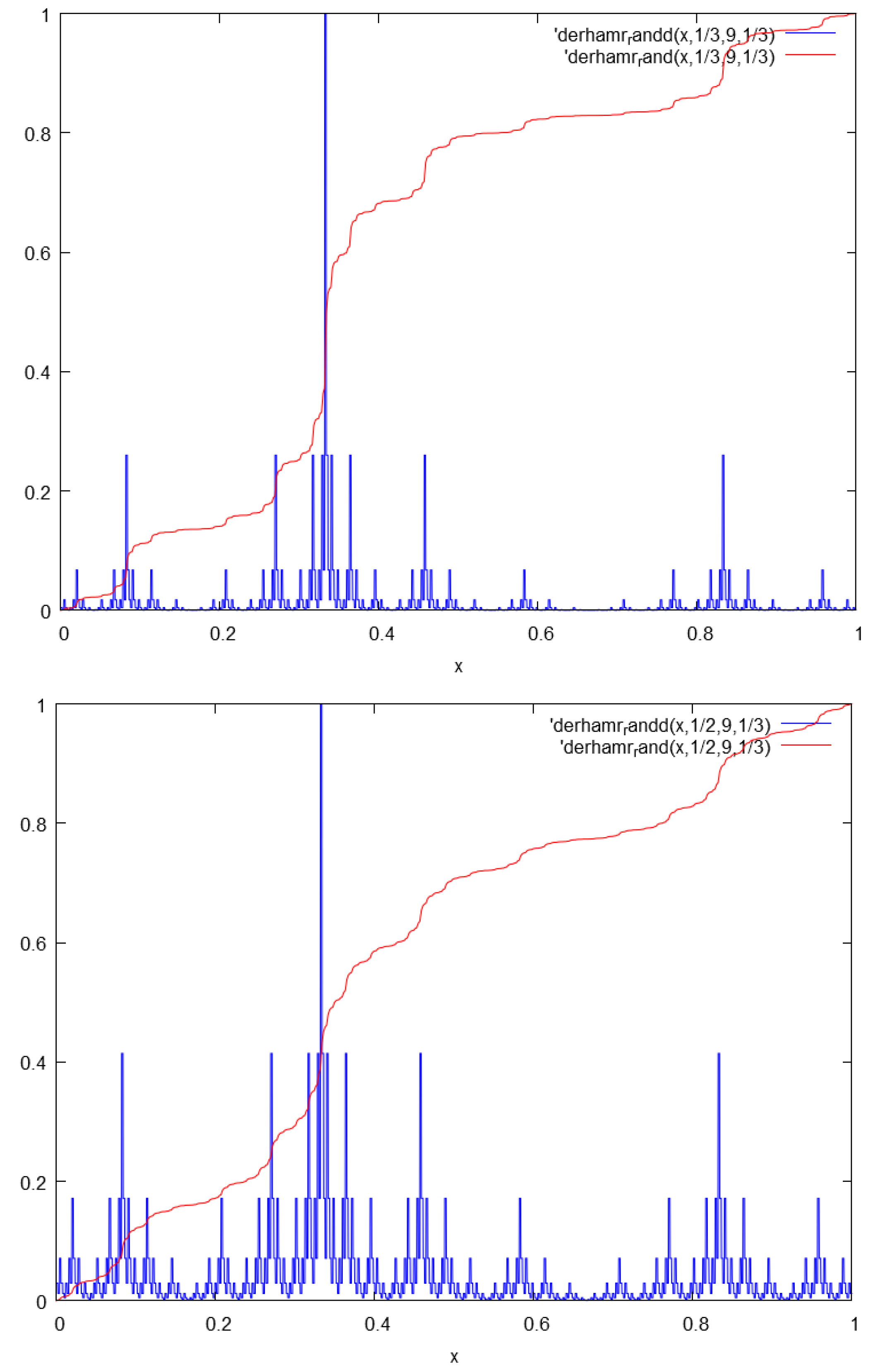
Therefore, either $a=1/2^{\beta }$ or $1-a=1/2^{\beta }$ so that ${\upsilon }_{+}^a{r}_0(x,a)=\mathbf{1}(x=0)$. The velocity can be computed algorithmically to arbitrary precision (Figure 2).

3.2.4. Langevin Evolution

Consider a non-linear problem, where the continuous phase-space trajectory of a system is represented by a F-analytic function $x\left(t\right)$ and t is a real-valued parameter, for example time or curve length. That is, suppose that a generalized Langevin equation holds uniformly in $[t,t+ϵ]$ for measurable functions a,B :

$${\Delta }_{ϵ}^{+}\left[x\right]\left(t\right)=a(x,t)ϵ+B(x,t){ϵ}^{\beta }+\mathcal{O}\left(ϵ\right),\beta \le 1$$

The form of the equation depends critically on the assumption of continuity of the reconstructed trajectory. This in turn demands for the fluctuations of the fractional term to be discontinuous. The proof technique is introduced in [24], while the argument is similar to the one presented in [32].

By hypothesis $\exists K$, such that $|{\Delta }_{ϵ}X|\le K{ϵ}^{\beta }$ and $x\left(t\right)$ is ${\mathbb{H}}^{\beta }$ . Therefore, without loss of generality we can set $a=0$ and apply the argument from [24]. Fix the interval $[t,t+ϵ]$ and choose a partition of points $\{t_k=t+k/Nϵ\}$ for an integral N.

$$x_{t_k}=x_{t_{k-1}}+B(x_{t_{k-1}},t_{k-1}){\left(ϵ/N\right)}^{\beta }+\mathcal{O}\left({ϵ}^{\beta }\right)$$

where we have set $x_{t_k}\equiv x\left(t_k\right)$. Therefore,

$${\Delta }_{ϵ}x=\frac{1}{N^{\beta }}\sum _{k=0}^{N-1}B(x_{t_k},t_k){ϵ}^{\beta }+\mathcal{O}\left({ϵ}^{\beta }\right)$$

Therefore, if we suppose that B is continuous in x or t after taking limit on both sides we arrive at

$$\underset{ϵ\to 0}{lim\; sup}\frac{{\Delta }_{ϵ}x}{{ϵ}^{\beta }}=B(x_t,t)=\frac{1}{N^{\beta }}\sum _{k=0}^{N-1}\underset{ϵ\to 0}{lim\; sup}B(x_{t_k},t_k)=N^{1-\beta }B(x_t,t)$$

so that $(1-N^{1-\beta })B(x,t)=0$. Therefore, either $\beta =1$ or $B(x,t)=0$. So that $B(x,t)$ must oscillate and is not continuous if $\beta <1$.

3.2.5. Brownian Motion

The presentation of this example follows [33]. However, in contrast to Zili ${\upsilon }_{+}^{\alpha }={\upsilon }_{-}^{\alpha }$ is not assumed point-wise. Consider the Brownian motion $W_t$. Using the stationarity and self-similarity of the increments ${\Delta }_{ϵ}^{+}{W}_t=\sqrt{ϵ}N(0,1)$ where $N(0,1)$ is a Gaussian random variable. Therefore,

$${\upsilon }_{\pm }^{\alpha }{W}_t=0,\alpha <1/2$$

while ${\upsilon }_{\pm }^{\alpha }{W}_t$ does not exist for $\alpha >1/2$ with probability $\mathbb{P}=1$. The estimate holds a.s. since $\mathbb{P}({\Delta }_{ϵ}^{+}{W}_t=0)=0$. Interestingly, for $\alpha =1/2$ the velocity can be regularized to a finite value if we take the expectation. That is

$${\upsilon }_{+}^{\alpha }\mathbb{E}{W}_t=0$$

since ${\Delta }_{ϵ}^{+}\mathbb{E}{W}_t=0$. Also ${\upsilon }_{+}^{\alpha }\mathbb{E}|W_t|=1$.

4. Characterization of Kolwankar-Gangal Local Fractional Derivatives

The overlap of the definitions of the Cherebit’s fractional velocity and the Kolwankar-Gangal fractional derivative is not complete [34]. Notably, Kolwankar-Gangal fractional derivatives are sensitive to the critical local Hölder exponents, while the fractional velocities are sensitive to the critical point-wise Hölder exponents and there is no complete equivalence between those quantities [35]. In this section we will characterize the local fractional derivatives in the sense of Kolwankar and Gangal using the notion of fractional velocity.

4.1. Fractional Integrals and Derivatives

The left Riemann-Liouville differ-integral of order $\beta \ge 0$ is defined as

$${}_{a+}{\mathbf{I}}_x^{\beta }f\left(x\right)={\displaystyle \frac{1}{\mathsf{\Gamma }\left(\beta \right)}}{\int }_a^{x}f\left(t\right){\left(x-t\right)}^{\beta -1}dt$$

while the right integral is defined as

$${}_{-a}{\mathbf{I}}_x^{\beta }f\left(x\right)={\displaystyle \frac{1}{\mathsf{\Gamma }\left(\beta \right)}}{\int }_x^{a}f\left(t\right){\left(t-x\right)}^{\beta -1}dt$$

where $\mathsf{\Gamma }\left(x\right)$ is the Euler’s Gamma function (Samko et al. [36], p. 33). The left (resp. right) Riemann- Liouville (R-L) fractional derivatives are defined as the expressions (Samko et al. [36], p. 35):

$$\begin{array}{cc}\hfill {\mathcal{D}}_{a+}^{\beta }f\left(x\right)& :=\frac{d}{dx}{}_{a+}{\mathbf{I}}_x^{1-\beta }f\left(x\right)=\frac{1}{\mathsf{\Gamma }(1-\beta )}\frac{d}{dx}{\int }_a^x\frac{f\left(t\right)}{{\left(x-t\right)}^{\beta }}dt\hfill \\ \hfill {\mathcal{D}}_{-a}^{\beta }f\left(x\right)& :=-\frac{d}{dx}{}_{-a}{\mathbf{I}}_x^{1-\beta }f\left(x\right)=-\frac{1}{\mathsf{\Gamma }(1-\beta )}\frac{d}{dx}{\int }_x^a\frac{f\left(t\right)}{{\left(t-x\right)}^{\beta }}dt\hfill \end{array}$$

The left (resp. right) R-L derivative of a function f exists for functions representable by fractional integrals of order $\alpha$ of some Lebesgue-integrable function. This is the spirit of the definition of Samko et al. ([36], Definition 2.3, p. 43) for the appropriate functional spaces:

$$\begin{array}{cc}\hfill {\mathcal{I}}_{a,+}^{\alpha }\left(L^1\right)& :=\left\{f:{}_{a+}{\mathbf{I}}_x^{\alpha }f\left(x\right)\in AC\left([a,b]\right),f\in L^1\left([a,b]\right),x\in [a,b]\right\},\hfill \\ \hfill {\mathcal{I}}_{a,-}^{\alpha }\left(L^1\right)& :=\left\{f:{}_{-a}{\mathbf{I}}_x^{\alpha }f\left(x\right)\in AC\left([a,b]\right),f\in L^1\left([a,b]\right),x\in [a,b]\right\}\hfill \end{array}$$

Here $AC$ denotes absolute continuity on an interval in the conventional sense. Samko et al. comment that the existence of a summable derivative $f^{\prime }\left(x\right)$ of a function $f\left(x\right)$ does not yet guarantee the restoration of $f\left(x\right)$ by the primitive in the sense of integration and go on to give references to singular functions for which the derivative vanishes almost everywhere and yet the function is not constant, such as for example, the De Rhams’s function [37].

To ensure restoration of the primitive by fractional integration, based on Th. 2.3 Samko et al. introduce another space of summable fractional derivatives, for which the Fundamental Theorem of Fractional Calculus holds.

Definition 4.

Define the functional spaces of summable fractional derivatives Samko et al. ([36], Definition 2.4, p. 44) as $E_{a,\pm }^{\alpha }\left([a,b]\right):=\left\{f:{\mathcal{I}}_{a,\pm }^{1-\alpha }\left(L^1\right)\right\}$.

In this sense

$${}_{a+}{\mathbf{I}}_x^{\alpha }\left({\mathcal{D}}_{a+}^{\alpha }f\right)\left(x\right)=f\left(x\right)$$

for $f\in E_{a,+}^{\alpha }\left([a,b]\right)$ (Samko et al. [36], Theorem 4, p. 44). While

$${\mathcal{D}}_{a+}^{\alpha }\left({}_{a+}{\mathbf{I}}_x^{\alpha }f\right)\left(x\right)=f\left(x\right)$$

for $f\in {\mathcal{I}}_{a,+}^{\alpha }\left(L^1\right)$.

So defined spaces do not coincide. The distinction can be seen from the following example:

Example 1.

Define

$$h\left(x\right):=\left\{\begin{array}{cc}0,\hfill & x\le 0\hfill \\ x^{\alpha -1},\hfill & x>0\hfill \end{array}\right.$$

for $0<\alpha <1$. Then ${}_{0+}{\mathbf{I}}_x^{1-\alpha }h\left(x\right)=\mathsf{\Gamma }\left(\alpha \right)$ for $x>0$ so that ${\mathcal{D}}_{0+}^{\alpha }h\left(x\right)=0$ everywhere in ${\mathbb{R}}^{}$.

On the other hand,

$${}_{0+}{\mathbf{I}}_x^{\alpha }h\left(x\right)=\frac{\mathsf{\Gamma }\left(\alpha \right)}{\mathsf{\Gamma }\left(2\alpha \right)}{x}^{2\alpha -1}$$

for $x>0$ and

$$\frac{\mathsf{\Gamma }\left(\alpha \right)}{\mathsf{\Gamma }\left(2\alpha \right)}{\mathcal{D}}_{0+}^{\alpha }{x}^{2\alpha -1}=x^{\alpha -1}.$$

Therefore, the fundamental theorem fails. It is easy to demonstrate that $h\left(x\right)$ is not $AC$ on any interval involving 0.

Therefore, the there is an inclusion $E_{a,+}^{\alpha }\subset {\mathcal{I}}_{a,+}^{\alpha }$.

4.2. The Local(ized) Fractional Derivative

The definition of local fractional derivative (LFD) introduced by Kolwankar and Gangal [38] is based on the localization of Riemann-Liouville fractional derivatives towards a particular point of interest in a way similar to Caputo.

Definition 5.

Define left LFD as

$${\mathcal{D}}_{KG+}^{\beta }f\left(x\right):=\underset{x\to a}{\lim }{\mathcal{D}}_{a+}^{\beta }\left[f-f\left(a\right)\right]\left(x\right)$$

and right LFD as

$${\mathcal{D}}_{KG-}^{\beta }f\left(x\right):=\underset{x\to a}{\lim }{\mathcal{D}}_{-a}^{\beta }\left[f\left(a\right)-f\right]\left(x\right).$$

Remark 4.

The seminal publication defined only the left derivative. Note that the LFD is more restrictive than the R-L derivative because the latter may not have a limit as $x\to a$.

Ben Adda and Cresson [23] and later Chen et al. [26] claimed that the Kolwankar—Gangal definition of local fractional derivative is equivalent to Cherbit’s definition for certain classes of functions. On the other hand, some inaccuracies can be identified in these articles [26,34]. Since the results of Chen et al. [26] and Ben Adda-Cresson [34] are proven under different hypotheses and notations I feel that separate proofs of the equivalence results using the theory established so-far are in order.

Proposition 5

(LFD equivalence). Let $f\left(x\right)$ be β-differentiable about x. Then ${\mathcal{D}}_{KG,\pm }^{\beta }f\left(x\right)$ exists and

$${\mathcal{D}}_{KG,\pm }^{\beta }f\left(x\right)=\mathsf{\Gamma }(1+\beta ){\upsilon }_{\pm }^{\beta }f\left(x\right).$$

Proof. 

We will assume that $f\left(x\right)$ is non-decreasing in the interval $[a,a+x]$. Since x will vary, for simplicity let’s assume that ${\upsilon }_{+}^{\beta }f\left(a\right)\in {\chi }_{}^{\beta }$. Then by Proposition 1 we have

$$f\left(z\right)=f\left(a\right)+{\upsilon }_{+}^{\beta }f\left(a\right){(z-a)}^{\beta }+\mathcal{O}\left({(z-a)}^{\beta }\right),a\le z\le x.$$

Standard treatments of the fractional derivatives [8] and the changes of variables $u=(t-a)/(x-a)$ give the alternative Euler integral formulation

$${\mathcal{D}}_{+a}^{\beta }f\left(x\right)=\frac{\partial }{\partial h}\left(\frac{h^{1-\beta }}{\mathsf{\Gamma }(1-\beta )}\underset{0}{\overset{1}{\int }}\frac{f(hu+a)-f\left(a\right)}{{(1-u)}^{\beta }}du\right)$$

(5)

for $h=x-a$. Therefore, we can evaluate the fractional Riemann-Liouville integral as follows:

$$\frac{h^{1-\beta }}{\mathsf{\Gamma }(1-\beta )}\underset{0}{\overset{1}{\int }}\frac{f(hu+a)-f\left(a\right)}{{(1-u)}^{\beta }}du=\frac{h^{1-\beta }}{\mathsf{\Gamma }(1-\beta )}\underset{0}{\overset{1}{\int }}\frac{K{\left(hu\right)}^{\beta }+\mathcal{O}\left({\left(hu\right)}^{\beta }\right)}{{(1-u)}^{\beta }}du=:I$$

setting conveniently $K={\upsilon }_{+}^{\beta }f\left(a\right)$. The last expression I can be evaluated in parts as

$$I=\underset{A}{\underbrace{{\displaystyle \frac{h^{1-\beta }}{\mathsf{\Gamma }(1-\beta )}}\underset{0}{\overset{1}{\int }}\frac{K{h}^{\beta }{u}^{\beta }}{{(1-u)}^{\beta }}du}}+\underset{C}{\underbrace{{\displaystyle \frac{h^{1-\beta }}{\mathsf{\Gamma }(1-\beta )}}\underset{0}{\overset{1}{\int }}\frac{\mathcal{O}\left({\left(hu\right)}^{\beta }\right)}{{(1-u)}^{\beta }}du}}.$$

The first expression is recognized as the Beta integral [8]:

$$A=\frac{h^{1-\beta }}{\mathsf{\Gamma }(1-\beta )}B\left(1-\beta ,1+\beta \right)h^{\beta }K=\mathsf{\Gamma }(1+\beta )Kh$$

In order to evaluate the second expression we observe that by Proposition 1

$$\left|\mathcal{O}\left({\left(hu\right)}^{\beta }\right)\right|\le \gamma {\left(hu\right)}^{\beta }$$

for a positive $\gamma ={\mathcal{O}}_1$. Assuming without loss of generality that $f\left(x\right)$ is non decreasing in the interval we have $C\le \mathsf{\Gamma }(1+\beta )\gamma h$ and

$${\mathcal{D}}_{a+}^{\beta }f\left(x\right)\le \left(K+\gamma \right)\mathsf{\Gamma }(1+\beta )$$

and the limit gives $\underset{x\to a+}{\lim }K+\gamma =K$ by the squeeze lemma and Proposition 1. Therefore, ${\mathcal{D}}_{KG+}^{\beta }f\left(a\right)=\mathsf{\Gamma }(1+\beta ){\upsilon }_{+}^{\beta }f\left(a\right)$. On the other hand, for ${\mathbb{H}}^{r,\alpha }$ and $\alpha >\beta$ by the same reasoning

$$A=\frac{h^{1-\beta }}{\mathsf{\Gamma }(1-\beta )}B\left(1-\beta ,1+\alpha \right)h^{\alpha }K=\mathsf{\Gamma }(1+\beta )K{h}^{1-\beta +\alpha }.$$

Then differentiation by h gives

$$A_h^{\prime }=\frac{\mathsf{\Gamma }(1+\alpha )}{\mathsf{\Gamma }(1+\alpha -\beta )}K{h}^{\alpha -\beta }.$$

Therefore,

$${\mathcal{D}}_{KG+}^{\beta }f\left(x\right)\le \frac{\mathsf{\Gamma }(1+\alpha )}{\mathsf{\Gamma }(1+\alpha -\beta )}\left(K+\gamma \right)h^{\alpha -\beta }$$

by monotonicity in h. Therefore, ${\mathcal{D}}_{KG\pm }^{\beta }f\left(a\right)={\upsilon }_{\pm }^{\beta }f\left(a\right)=0$. Finally, for $\alpha =1$ the expression A should be evaluated as the limit $\alpha \to 1$ due to divergence of the $\mathsf{\Gamma }$ function. The proof for the left LFD follows identical reasoning, observing the backward fractional Taylor expansion property.

Proposition 6.

Suppose that ${\mathcal{D}}_{KG\pm }^{\beta }f\left(x\right)$ exists finitely and the related R-L derivative is summable in the sense of Definition 4. Then f is β-differentiable about x and ${\mathcal{D}}_{KG,\pm }^{\beta }f\left(x\right)=\mathsf{\Gamma }(1+\beta ){\upsilon }_{\pm }^{\beta }f\left(x\right)$.

Proof. 

Suppose that $f\in E_{a,+}^{\alpha }\left([a,a+\delta ]\right)$ and let ${\mathcal{D}}_{KG+}^{\alpha }f\left(x\right)=L$. The existence of this limit implies the inequality

$$\left|{\mathcal{D}}_{a+}^{\alpha }\left[f-f\left(a\right)\right]\left(x\right)-L\right|<\mu$$

for $|x-a|\le \delta$ and a Cauchy sequence $\mu$.

Without loss of generality suppose that ${\mathcal{D}}_{a+}^{\alpha }\left[f-f\left(a\right)\right]\left(x\right)$ is non-decreasing and $L\ne 0$. We proceed by integrating the inequality:

$${}_{a+}{\mathbf{I}}_x^{\alpha }\left({\mathcal{D}}_{a+}^{\alpha }\left[f-f\left(a\right)\right]\left(x\right)-L\right)<{}_{a+}{\mathbf{I}}_x^{\alpha }\mu$$

Then by the Fundamental Theorem

$$f\left(x\right)-f\left(a\right)-\frac{L}{\mathsf{\Gamma }\left(\alpha \right)}{(x-a)}^{\alpha }<\frac{\mu {(x-a)}^{\alpha }}{\mathsf{\Gamma }\left(\alpha \right)}$$

and

$$\frac{f\left(x\right)-f\left(a\right)-L/\mathsf{\Gamma }\left(\alpha \right)}{{(x-a)}^{\alpha }}<\frac{\mu }{\mathsf{\Gamma }\left(\alpha \right)}=\mathcal{O}\left(1\right)$$

which is Cauchy. Therefore, by Proposition 1 f is $\alpha$-differentiable at x and ${\mathcal{D}}_{KG,+}^{\alpha }f\left(x\right)=\mathsf{\Gamma }(1+\alpha ){\upsilon }_{+}^{\alpha }f\left(x\right)$. The last assertion comes from Proposition 5. The right case can be proven in a similar manner. ☐

The weaker condition of only point-wise Hölder continuity requires the additional hypothesis of summability as identified in [34]. The following results can be stated.

Lemma 1.

Suppose that ${\mathcal{D}}_{KG\pm }^{\beta }f\left(a\right)$ exists finitely in the weak sense, i.e., implying only that $f\in {\mathcal{I}}_{a,+}^{\alpha }\left(L^1\right)$. Then Condition C1 holds for f a.e. in the interval $[a,x+ϵ]$.

Proof. 

The left R-L derivative can be evaluated as follows. Consider the fractional integral in the Liouville form

$$\begin{array}{cc}\hfill I_1& =\underset{0}{\overset{ϵ+x-a}{\int }}\frac{f(x+ϵ-h)-f\left(a\right)}{h^{\beta }}dh-\underset{0}{\overset{x-a}{\int }}\frac{f(x-h)-f\left(a\right)}{h^{\beta }}dh\hfill \\ & =\underset{I_2}{\underbrace{\underset{x-a}{\overset{ϵ+x-a}{\int }}\frac{f(x+ϵ-h)-f\left(a\right)}{h^{\beta }}dh}}+\underset{I_3}{\underbrace{\underset{0}{\overset{x-a}{\int }}\frac{f(x+ϵ-h)-f(x-h)}{h^{\beta }}dh}}\hfill \end{array}$$

Without loss of generality assume that f is non-decreasing in the interval $[a,x+ϵ-a]$ and set $M_{y,x}={sup}_{[x,y]}f-f\left(x\right)$ and $m_{y,x}={inf}_{[x,y]}f-f\left(x\right)$. Then

$$I_2\le \underset{x-a}{\overset{ϵ+x-a}{\int }}\frac{M_{x+ϵ,a}}{h^{\beta }}dh=\frac{M_{x+ϵ,a}}{1-\beta }\left[{{\left(x-ϵ+a\right)}^{1-\beta }-\left(x-a\right)}^{1-\beta }\right]\le ϵ\frac{M_{x+ϵ,a}}{{\left(x-a\right)}^{\beta }}+\mathcal{O}\left({ϵ}^2\right)$$

for $x\ne a$. In a similar manner

$$I_2\ge m_{x+ϵ,a}\frac{ϵ}{{\left(x-a\right)}^{\beta }}+\mathcal{O}\left({ϵ}^2\right).$$

Then dividing by $ϵ$ gives

$$\frac{m_{x+ϵ,a}}{{\left(x-a\right)}^{\beta }}+\mathcal{O}\left(ϵ\right)\le \frac{I_2}{ϵ}\le \frac{M_{x+ϵ,a}}{{\left(x-a\right)}^{\beta }}+\mathcal{O}\left(ϵ\right)$$

Therefore, the quotient limit is bounded from both sides as

$$\frac{m_{x,a}}{{\left(x-a\right)}^{\beta }}\le \underset{I_2^{\prime }}{\underbrace{\underset{ϵ\to 0}{\lim }\frac{I_2}{ϵ}}}\le \frac{M_{x,a}}{{\left(x-a\right)}^{\beta }}$$

by the continuity of f. In a similar way we establish

$$\begin{array}{c}\hfill I_3\le \underset{0}{\overset{x-a}{\int }}\frac{M_{x+ϵ,x}}{h^{\beta }}dh=\frac{M_{x+ϵ,x}}{1-\beta }{\left(x-a\right)}^{1-\beta }\end{array}$$

and

$$\frac{m_{x+ϵ,x}}{1-\beta }{\left(x-a\right)}^{1-\beta }\le I_3$$

Therefore,

$$\frac{m_{x+ϵ,x}}{\left(1-\beta \right)ϵ}{\left(x-a\right)}^{1-\beta }\le \frac{I_3}{ϵ}\le \frac{M_{x+ϵ,x}}{\left(1-\beta \right)ϵ}{\left(x-a\right)}^{1-\beta }$$

By the absolute continuity of the integral the quotient limit $\frac{I_3}{ϵ}$ exists as $ϵ\to 0$ for almost all x. This also implies the existence of the other two limits. Therefore, the following bond holds

$$m_{x+ϵ,x}^{☆}\frac{{\left(x-a\right)}^{1-\beta }}{\left(1-\beta \right)}\le \underset{I_3^{\prime }}{\underbrace{\underset{ϵ\to 0}{\lim }\frac{I_3}{ϵ}}}\le M_{x+ϵ,x}^{☆}\frac{{\left(x-a\right)}^{1-\beta }}{\left(1-\beta \right)}$$

where $M_{x+ϵ,x}^{☆}={sup}_{[x,x+ϵ]}{f}^{\prime }$ and $m_{x+ϵ,x}^{☆}={inf}_{[x,x+ϵ]}{f}^{\prime }$ wherever these exist. Therefore, as x approaches a $\underset{x\to a}{\lim }{I}_3^{\prime }=0$.

Finally, we establish the bounds of the limit

$$\underset{x\to a}{\lim }\frac{m_{x,a}}{{\left(x-a\right)}^{\beta }}\le \underset{x\to a}{\lim }{I}_2^{\prime }\le \underset{x\to a}{\lim }\frac{M_{x,a}}{{\left(x-a\right)}^{\beta }}.$$

Therefore, Condition C1 is necessary for the existing of the limit and hence for $\underset{x\to a}{\lim }{I}^{\prime }$. ☐

Based on this result, we can state a generic continuity result for LFD of fractional order.

Theorem 3

(Continuity of LFD). For $0<\beta <1$ if ${\mathcal{D}}_{KG\pm }^{\beta }f\left(x\right)$ is continuous about x then ${\mathcal{D}}_{KG\pm }^{\beta }f\left(x\right)=0$.

Proof. 

We will prove the case for ${\mathcal{D}}_{KG+}^{\beta }f\left(x\right)$. Suppose that LFD is continuous in the interval $[a,x]$ and ${\mathcal{D}}_{KG+}^{\beta }f\left(a\right)=K\ne 0$. Then the conditions of Lemma 1 apply, that is $f\in {\mathbb{H}}^{\beta }$ a.e. in $[a,x]$. Therefore, without loss of generality we can assume that $f\in {\mathbb{H}}^{\beta }$ at a. Further, we express the R-L derivative in Euler form setting $z=x-a$ :

$${\mathcal{D}}_z^{\beta }f=\frac{\partial }{\partial z}\frac{z^{1-\beta }}{\mathsf{\Gamma }(1-\beta )}\underset{0}{\overset{1}{\int }}\frac{f\left(z(1-t)+a\right)-f\left(a\right)}{t^{\beta }}dt$$

By the monotonicity of the power function (e.g., Hölder growth property):

$$k_1\mathsf{\Gamma }(1+\beta )\le {\mathcal{D}}_z^{\beta }f\le K_1\mathsf{\Gamma }(1+\beta )$$

where $k_1={inf}_{[a,a+z]}f-f\left(a\right)$ and $K_1={sup}_{[a,a+z]}f-f\left(a\right)$. On the other hand, we can split the integrand in two expressions for an arbitrary intermediate value $z_0=\lambda z\le z$. This gives

$$\begin{array}{cc}\hfill {\mathcal{D}}_z^{\beta }f=\frac{\partial }{\partial z}& \frac{z^{1-\beta }}{\mathsf{\Gamma }(1-\beta )}\underset{0}{\overset{1}{\int }}\frac{f\left(z(1-t)+a\right)-f\left(\lambda z(1-t)+a\right)}{t^{\beta }}dt+\hfill \\ \hfill \frac{\partial }{\partial z}& \frac{z^{1-\beta }}{\mathsf{\Gamma }(1-\beta )}\underset{0}{\overset{1}{\int }}\frac{f\left(\lambda z(1-t)+a\right)-f\left(a\right)}{t^{\beta }}dt.\hfill \end{array}$$

Therefore, by the Hölder growth property and monotonicity in z

$${\mathcal{D}}_z^{\beta }f\le \frac{\partial }{\partial z}z{\left(1-\lambda \right)}^{\beta }\mathsf{\Gamma }(1+\beta )K_{1-\lambda }+\frac{\partial }{\partial z}z{\lambda }^{\beta }\mathsf{\Gamma }(1+\beta )K_{\lambda }.$$

where $K_{\lambda }={sup}_{[a,a+\lambda z]}f-f\left(a\right)$ and $K_{1-\lambda }={sup}_{[a+\lambda z,a+z]}f-f(a+\lambda z)$. Therefore,

$$k_1\mathsf{\Gamma }(1+\beta )\le {\mathcal{D}}_z^{\beta }f\le \left({\left(1-\lambda \right)}^{\beta }{K}_{1-\lambda }+{\lambda }^{\beta }{K}_{\lambda }\right)\mathsf{\Gamma }(1+\beta ).$$

However, by the assumption of continuity $k_1=K_{\lambda }=K_{1-\lambda }=K$ as $z\to 0$ and the non-strict inequalities become equalities so that

$$\left({\left(1-\lambda \right)}^{\beta }+{\lambda }^{\beta }-1\right)K=0.$$

However, if $\beta <1$ we have contradiction since then $\lambda =1$ or $\lambda =0$ must hold and $\lambda$ ceases to be arbitrary. Therefore, since $\lambda$ is arbitrary $K=0$ must hold. The right case can be proven in a similar manner. ☐

Corollary 3

(Discontinuous LFD). Let ${\chi }_{\beta }:=\{x:{\mathcal{D}}_{KG\pm }^{\beta }f\left(x\right)\ne 0\}$. Then for $0<\beta <1$ ${\chi }_{\beta }$ is totally disconnected.

Remark 5.

This result is related to Corollary 3 in [26] however here it is established in a more general way.

4.3. Equivalent Forms of LFD

LFD can be calculated in the following way. Starting from Formula (5) for convenience we define the integral average

$$M_a\left(h\right):=\underset{0}{\overset{1}{\int }}\frac{f(hu+a)-f\left(a\right)}{{(1-u)}^{\beta }}du$$

(6)

Then

$$\mathsf{\Gamma }(1-\beta ){\mathcal{D}}_{KG+}^{\beta }f\left(a\right)=\underset{h\to 0}{\lim }\underset{N_h}{\underbrace{h^{1-\beta }\frac{\partial }{\partial h}{M}_a\left(h\right)}}+\left(1-\beta \right)\underset{h\to 0}{\lim }\frac{M_a\left(h\right)}{h^{\beta }}$$

Then we apply L’Hôpital’s rule on the second term :

$$\mathsf{\Gamma }(1-\beta ){\mathcal{D}}_{KG+}^{\beta }f\left(a\right)=\underset{h\to 0}{\lim }{N}_h+\frac{1-\beta }{\beta }\underset{h\to 0}{\lim }\underset{N_h}{\underbrace{h^{1-\beta }\frac{\partial }{\partial h}{M}_a\left(h\right)}}=\frac{1}{\beta }\underset{h\to 0}{\lim }{N}_h$$

Finally,

$${\mathcal{D}}_{KG+}^{\beta }f\left(a\right)=\frac{1}{\beta \mathsf{\Gamma }(1-\beta )}\underset{h\to 0}{\lim }{h}^{1-\beta }\frac{\partial }{\partial h}\underset{0}{\overset{1}{\int }}\frac{f(hu+a)-f\left(a\right)}{{(1-u)}^{\beta }}du$$

(7)

From this equation there are two conclusions that can be drawn.

First, for $f\in L^1(a,x)$ by application of the definition of fractional velocity and L’Hôpital’s rule:

$${\mathcal{D}}_{KG+}^{\beta }f\left(a\right)=\frac{{\upsilon }_{+}^{\beta }{M}_a\left(0\right)}{\mathsf{\Gamma }(1-\beta )}$$

(8)

if the last limit exists. Therefore, LFD can be characterized in terms of fractional velocity. This can be formalized in the following proposition:

Proposition 7.

Suppose that $f\in {\mathcal{I}}_{a,\pm }^{\alpha }\left(L^1\right)$ for $x\in [a,a+\delta )$ (resp. $x\in (a-\delta ,a]$) for some small $\delta >0$. If ${\upsilon }_{\pm }^{\beta }{M}_a\left(0\right)$ exists finitely then

$${\mathcal{D}}_{KG\pm }^{\beta }f\left(a\right)=\frac{{\upsilon }_{\pm }^{\beta }{M}_a\left(0\right)}{\mathsf{\Gamma }(1-\beta )}$$

where $M_a\left(h\right)$ is given by Formula (6).

From this we see that f may not be $\beta$-differentiable at x. From this perspective LFD is a derived concept - it is the $\beta -$ velocity of the integral average.

Second, for BV functions the order of integration and parametric derivation can be exchanged so that

$${\mathcal{D}}_{KG+}^{\beta }f\left(a\right)=\frac{1}{\beta \mathsf{\Gamma }(1-\beta )}\underset{h\to 0}{\lim }{h}^{1-\beta }\underset{0}{\overset{1}{\int }}\frac{u{f}^{\prime }(hu+a)}{{(1-u)}^{\beta }}du$$

(9)

where we demand the existence of $f^{\prime }\left(x\right)$ a.e in $(a,x)$, which follows from the Lebesgue differentiation theorem. This statement can be formalized as.

Proposition 8.

Suppose that $f\in BV(a,\delta ]$ for some small $\delta >0$. Then

$${\mathcal{D}}_{KG+}^{\beta }f\left(a\right)=\frac{1}{\beta \mathsf{\Gamma }(1-\beta )}\underset{h\to 0}{\lim }{h}^{1-\beta }\underset{0}{\overset{1}{\int }}\frac{u{f}^{\prime }(hu+a)}{{(1-u)}^{\beta }}du$$

In the last two formulas we can also set $\mathsf{\Gamma }(-\beta )=\beta \mathsf{\Gamma }(1-\beta )$ by the reflection formula.

Therefore, in the conventional form for a BV function

$${\mathcal{D}}_{KG+}^{\beta }f\left(a\right)=\frac{1}{\beta \mathsf{\Gamma }(1-\beta )}\underset{x\to a+}{\lim }{(x-a)}^{1-\beta }\frac{\partial }{\partial x}\underset{0}{\overset{1}{\int }}\frac{f\left(\right(x-a)u+a)-f\left(a\right)}{{(1-u)}^{\beta }}du$$

(10)

5. Discussion

Kolwankar-Gangal local fractional derivative was introduced as tools for the study of the scaling of physical systems and systems exhibiting fractal behavior [39]. The conditions for applicability of the K-G fractional derivative were not specified in the seminal paper, which leaves space for different interpretations and sometimes confusions. For example, recently Tarasov claimed that local fractional derivatives of fractional order vanish everywhere [40]. In contrast, the results presented here demonstrate that local fractional derivatives vanish only if they are continuous. Moreover, they are non-zero on arbitrary dense sets of measure zero for $\beta$-differentiable functions as shown.

Another confusion is the initial claim presented in [23] that K-G fractional derivative is equivalent to what is called here $\beta$-fractional velocity. This needed to be clarified in [26] and restricted to the more limited functional space of summable fractional Riemann-Liouville derivatives [34].

Presented results call for a careful inspection of the claims branded under the name of “local fractional calculus” using K-G fractional derivative. Specifically, in the implied conditions on image function’s regularity and arguments of continuity of resulting local fractional derivative must be examined in all cases. For example, in another stream of literature fractional difference quotients are defined on fractal sets, such as the Cantor’s set [41]. This is not to be confused with the original approach of Cherebit, Kolwankar and Gangal where the topology is of the real line and the set ${\chi }_{\alpha }$ is totally disconnected.

6. Conclusions

As demonstrated here, fractional velocities can be used to characterize the set of change of F-analytic functions. Local fractional derivatives and the equivalent fractional velocities have several distinct properties compared to integer-order derivatives. This may induce some wrong expectations to uninitiated reader. Some authors can even argue that these concepts are not suitable tools to deal with non-differentiable functions. However, this view pertains only to expectations transfered from the behavior of ordinary derivatives. On the contrary, one-sided local fractional derivatives can be used as a tool to study local non-linear behavior of functions as demonstrated by the presented examples. In applied problems, local fractional derivatives can be also used to derive fractional Taylor expansions [24,42,43].

References

- Mandelbrot, B. Fractal Geometry of Nature; Henry Holt & Co.: New York, NY, USA, 1982. [Google Scholar]
- Mandelbrot, B. Les Objets Fractals: Forme, Hasard et Dimension; Flammarion: Paris, France, 1989. [Google Scholar]
- Metzler, R.; Klafter, J. The restaurant at the end of the random walk: Recent developments in the description of anomalous transport by fractional dynamics. J. Phys. A Math. Gen. 2004, 37, R161–R208. [Google Scholar] [CrossRef]
- Wheatcraft, S.W.; Meerschaert, M.M. Fractional conservation of mass. Adv. Water Resour. 2008, 31, 1377–1381. [Google Scholar] [CrossRef]
- Caputo, M.; Mainardi, F. Linear models of dissipation in anelastic solids. Rivista del Nuovo Cimento 1971, 1, 161–198. [Google Scholar] [CrossRef]
- Mainardi, F. Fractional Calculus: Some Basic Problems in Continuum and Statistical Mechanics. In Fractals and Fractional Calculus in Continuum Mechanics; Springer: Wien, Austria; New York, NY, USA, 1997; pp. 291–348. [Google Scholar]
- Gorenflo, R.; Mainardi, F. Continuous time random walk, Mittag-Leffler waiting time and fractional diffusion: Mathematical aspects. In Anomalous Transport; Wiley-VCH Verlag GmbH & Co. KGaA: Weinheim, Germany, 2008; pp. 93–127. [Google Scholar]
- Oldham, K.B.; Spanier, J.S. The Fractional Calculus: Theory and Applications of Differentiation and Integration to Arbitrary Order; Academic Press: New York, NY, USA, 1974. [Google Scholar]
- Schroeder, M. Fractals, Chaos, Power Laws: Minutes from an Infinite Paradise; Dover Publications: Mineola, NY, USA, 1991. [Google Scholar]
- Losa, G.; Nonnenmacher, T. Self-similarity and fractal irregularity in pathologic tissues. Mod. Pathol. 1996, 9, 174–182. [Google Scholar] [PubMed]
- Darst, R.; Palagallo, J.; Price, T. Curious Curves; World Scientific Publishing Company: Singapore, 2009. [Google Scholar]
- John Hutchinson. Fractals and self similarity. Indiana Univ. Math. J. 1981, 30, 713–747. [Google Scholar]
- Mandelbro, B.B. Intermittent Turbulence in Self-Similar Cascades: Divergence of High Moments and Dimension of the Carrier; Springer: New York, NY, USA, 1999; pp. 317–357. [Google Scholar]
- Meneveau, C.; Sreenivasan, K.R. Simple multifractal cascade model for fully developed turbulence. Phys. Rev. Lett. 1987, 59, 1424–1427. [Google Scholar]
- Sreenivasan, K.R.; Meneveau, C. The fractal facets of turbulence. J. Fluid Mech. 1986, 173, 357–386. [Google Scholar] [CrossRef]
- Puente, C.; López, M.; Pinzón, J.; Angulo, J. The gaussian distribution revisited. Adv. Appl. Probab. 1996, 28, 500–524. [Google Scholar] [CrossRef]
- Nottale, L. Scale relativity and fractal space-time: Theory and applications. Found. Sci. 2010, 15, 101–152. [Google Scholar] [CrossRef]
- Cresson, J.; Pierret, F. Multiscale functions, scale dynamics, and applications to partial differential equations. J. Math. Phys. 2016, 57, 053504. [Google Scholar] [CrossRef]
- Cherbit, G. Local dimension, momentum and trajectories. In Fractals, Non-Integral Dimensions and Applications; John Wiley & Sons: Paris, France, 1991; pp. 231–238. [Google Scholar]
- Prodanov, D. Characterization of strongly non-linear and singular functions by scale space analysis. Chaos Solitons Fractals 2016, 93, 14–19. [Google Scholar] [CrossRef]
- Du Bois-Reymond, P. Versuch einer classification der willkürlichen functionen reeller argumente nach ihren aenderungen in den kleinsten intervallen. J. Reine Angew. Math. 1875, 79, 21–37. [Google Scholar]
- Faber, G. Über stetige funktionen. Math. Ann. 1909, 66, 81–94. [Google Scholar] [CrossRef]
- Ben Adda, F.; Cresson, J. About non-differentiable functions. J. Math. Anal. Appl. 2001, 263, 721–737. [Google Scholar] [CrossRef]
- Prodanov, D. Conditions for continuity of fractional velocity and existence of fractional Taylor expansions. Chaos Solitons Fractals 2017, 102, 236–244. [Google Scholar] [CrossRef]
- Odibat, Z.M.; Shawagfeh, N.T. Generalized Taylor’s formula. Appl. Math. Comput. 2007, 186, 286–293. [Google Scholar] [CrossRef]
- Chen, Y.; Yan, Y.; Zhang, K. On the local fractional derivative. J. Math. Anal. Appl. 2010, 362, 17–33. [Google Scholar] [CrossRef]
- Lomnicki, Z.; Ulam, S. Sur la théorie de la mesure dans les espaces combinatoires et son application au calcul des probabilités i. variables indépendantes. Fundam. Math. 1934, 23, 237–278. [Google Scholar] [CrossRef]
- Cesàro, E. Fonctions continues sans dérivée. Arch. Math. Phys. 1906, 10, 57–63. [Google Scholar]
- Salem, R. On some singular monotonic functions which are strictly increasing. Trans. Am. Math. Soc. 1943, 53, 427–439. [Google Scholar]
- Berg, L.; Krüppel, M. De rham’s singular function and related functions. Zeitschrift für Analysis und Ihre Anwendungen 2000, 19, 227–237. [Google Scholar]
- Neidinger, R. A fair-bold gambling function is simply singular. Am. Math. Mon. 2016, 123, 3–18. [Google Scholar] [CrossRef]
- Gillespie, D.T. The mathematics of Brownian motion and Johnson noise. Am. J. Phys. 1996, 64, 225–240. [Google Scholar] [CrossRef]
- Zili, M. On the mixed fractional brownian motion. J. Appl. Math. Stoch. Anal. 2006, 2006, 32435. [Google Scholar] [CrossRef]
- Ben Adda, F.; Cresson, J. Corrigendum to “About non-differentiable functions”. J. Math. Anal. Appl. 2013, 408, 409–413. [Google Scholar] [CrossRef]
- Kolwankar, K.M.; Lévy Véhel, J. Measuring functions smoothness with local fractional derivatives. Fract. Calc. Appl. Anal. 2001, 4, 285–301. [Google Scholar]
- Samko, S.; Kilbas, A.; Marichev, O. Fractional Integrals and Derivatives: Theory and Applications; Gordon and Breach: Yverdon, Switzerland, 1993. [Google Scholar]
- De Rham, G. Sur quelques courbes definies par des equations fonctionnelles. Rendiconti del Seminario Matematico Università e Politecnico di Torino 1957, 16, 101–113. [Google Scholar]
- Kolwankar, K.M.; Gangal, A.D. Fractional differentiability of nowhere differentiable functions and dimensions. Chaos 1996, 6, 505–513. [Google Scholar] [CrossRef] [PubMed]
- Kolwankar, K.M.; Gangal, A.D. Local fractional Fokker-Planck equation. Phys. Rev. Lett. 1998, 80, 214–217. [Google Scholar] [CrossRef]
- Tarasov, V.E. Local fractional derivatives of differentiable functions are integer-order derivatives or zero. Int. J. Appl. Comput. Math. 2016, 2, 195–201. [Google Scholar] [CrossRef]
- Yang, X.J.; Baleanu, D.; Srivastava, H.M. Local Fractional Integral Transforms and Their Applications; Academic Press: Cambridge, MA, USA, 2015. [Google Scholar]
- Liu, Z.; Wang, T.; Gao, G. A local fractional Taylor expansion and its computation for insufficiently smooth functions. East Asian J. Appl. Math. 2015, 5, 176–191. [Google Scholar] [CrossRef]
- Prodanov, D. Regularization of derivatives on non-differentiable points. J. Phys. Conf. Ser. 2016, 701, 012031. [Google Scholar] [CrossRef]
- Prodanov, D. Fractional variation of Hölderian functions. Fract. Calc. Appl. Anal. 2015, 18, 580–602. [Google Scholar] [CrossRef]
Figure 1.
Recursive construction of the Neidinger’s function; iteration levels 2, 4, 8.
Figure 2.
Approximation of the fractional velocity of Neidinger’s function. Recursive construction of the fractional velocity for (top) and (bottom), iteration level 9. The Neidinger’s function IFS are given for comparison for the same iteration level.
© 2018 by the author. Licensee MDPI, Basel, Switzerland. This article is an open access article distributed under the terms and conditions of the Creative Commons Attribution (CC BY) license (http://creativecommons.org/licenses/by/4.0/).
Share and Cite
MDPI and ACS Style
Prodanov, D. Fractional Velocity as a Tool for the Study of Non-Linear Problems. Fractal Fract. 2018, 2, 4. https://doi.org/10.3390/fractalfract2010004
AMA Style
Prodanov D. Fractional Velocity as a Tool for the Study of Non-Linear Problems. Fractal and Fractional. 2018; 2(1):4. https://doi.org/10.3390/fractalfract2010004
Chicago/Turabian StyleProdanov, Dimiter. 2018. "Fractional Velocity as a Tool for the Study of Non-Linear Problems" Fractal and Fractional 2, no. 1: 4. https://doi.org/10.3390/fractalfract2010004