Comparison between the Second and Third Generations of the CRONE Controller: Application to a Thermal Diffusive Interface Medium

Abstract

The control of thermal interfaces has gained importance in recent years because of the high cost of heating and cooling materials in many applications. Thus, the main focus in this work is to compare the second and third generations of the CRONE controller (French acronym of Commande Robuste d’Ordre Non Entier), which means a non-integer order robust controller, and to synthesize a robust controller that can fit several types of systems. For this study, the plant consists of a rectangular homogeneous bar of length L, where the heating element in applied on one boundary, and a temperature sensor is placed at distance x from that boundary (x is considered very small with respect to L). The type of material used is the third parameter, which may help in analyzing the robustness of the synthesized controller. The originality of this work resides in controlling a non-integer plant using a fractional order controller, as, so far, almost all of the systems where the CRONE controller has been implemented were of integer order. Three case studies were defined in order to show how and where each CRONE generation controller can be applied. These case studies were chosen in such a way as to influence the asymptotic behavior of the open-loop transfer function in the Black–Nichols diagram in order to point out the importance of respecting the conditions of the applications of the CRONE generations. Results show that the second generation performs well when the parametric uncertainties do not affect the phase of the plant, whereas the third generation is the most robust, even when both the phase and the gain variations are encountered. However, it also has some limitations, especially when the temperature to be controlled is far from the interface when the density of flux is applied.

1. Introduction

The thermal application is a common application for control. It is used in several engineering domains as the heating/cooling of houses [1,2], the control of the temperature inside the car [3,4] or in the industrial machinery [5], and much more. In more details, the work in this field started in the 1940s with the works of Jones [6] and a group of American electrical engineers [7]. Then, in the 1950s, the researchers were more involved in the control of thermal neutron reactors [8,9] and electric cables dissipation [10,11]. These studies had increased since the end of the previous decade, when the scientists stopped focusing on the study of the material properties, and started searching for more ecological systems to control the temperature within the building in order to reduce the oil and fuel usage [12,13].

However, the work on diffusive interfaces was launched in the late 1970s and 1980s with the works of Kumar, who modeled the thermal boundaries near an oil plant [14]. As for the others, they worked on the modeling of diffusive interfaces at furnaces [15], boilers [16] and some geometric shapes representing the separation medium [17,18]. In the last decade of the twentieth century, this domain was investigated by lots of researchers who demonstrated that the relation between the input flux and the output temperature is of a fractional order. From among them, we can recognize the remarkable works of Trigeassou and his team [19,20,21], Battablia [22,23], the CRONE team of Bordeaux university [24,25,26], the relevant modeling approach based on the space-fractional continuum models [27,28,29], and much more.

As for the control, it was applied a long time ago, even before Christ, when Ktesibios (270 B.C.) implemented the water clocks working on feedback control [30]. The contemporary control theory was effectively launched in the middle of the twentieth century with the remarkable work of Bode, Nichols, and Nyquist [31]. In its first years, the integer and linear order systems were treated on both time and frequency domains.

As for fractional theory, it is relatively an old idea that dates back to the end of the seventieth century, when some letters were exchanged between two well-known mathematicians at that epoch, L’Hopital and Leibnitz in which they asked each other about the meaning of a derivative of order 0.5 [32]. Many mathematicians defined this type of derivative/integration as Liouville, Caputo, and Riemann [33]. Nevertheless, these calculations remained theoretical until the last quarter of the twentieth century, when Oustaloup was the first to design a fractional control of order 3/2 to control a laser beam [34]. He was one of the first researchers to introduce the fractional calculus in engineering domain applications [35,36,37,38]. Due to the obtained results, many other contributions appeared from Ortigueira [39,40], Machado [41,42], and Vinagre [43,44].

Hence, this paper will present the control of a diffusive interface medium, consisting of a homogeneous rectangular finite rod, by the CRONE controller. The novelty of this work is that it presents a fractional order plant that will be controlled by a fractional order controller, who will be, for the first time, real (when applying the second generation CRONE), and in a second time, this controller will be complex (by applying the third generation CRONE). Added to that, the robustness of these controllers will be studied when varying the bar metal, the position of the point where the temperature is to be measured, the length of the bar, and so on. Thus, three case studies will be shown in order to show the behavior of the open-loop system, and to indicate the conditions of application for each CRONE generation. Since the objective of this paper is to point out the importance of applying the CRONE controller to a fractional order plant, we were not interested in comparing the performance of this controller to other ones.

For the remaining part of this paper, we will consider that the length of the bar is much more important than the position of the temperature sensor. As for the user specifications, two main constraints will be considered hereafter:

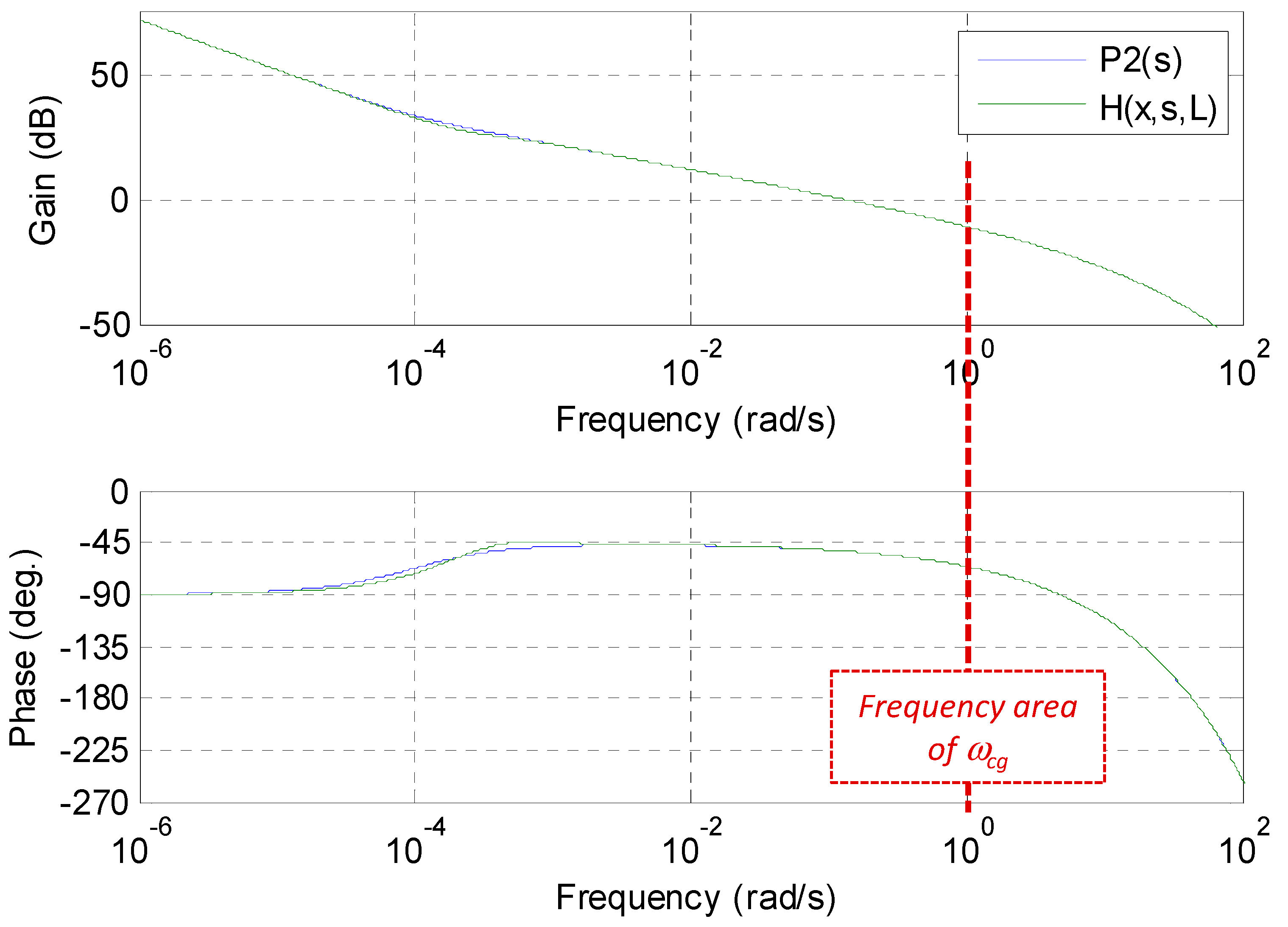
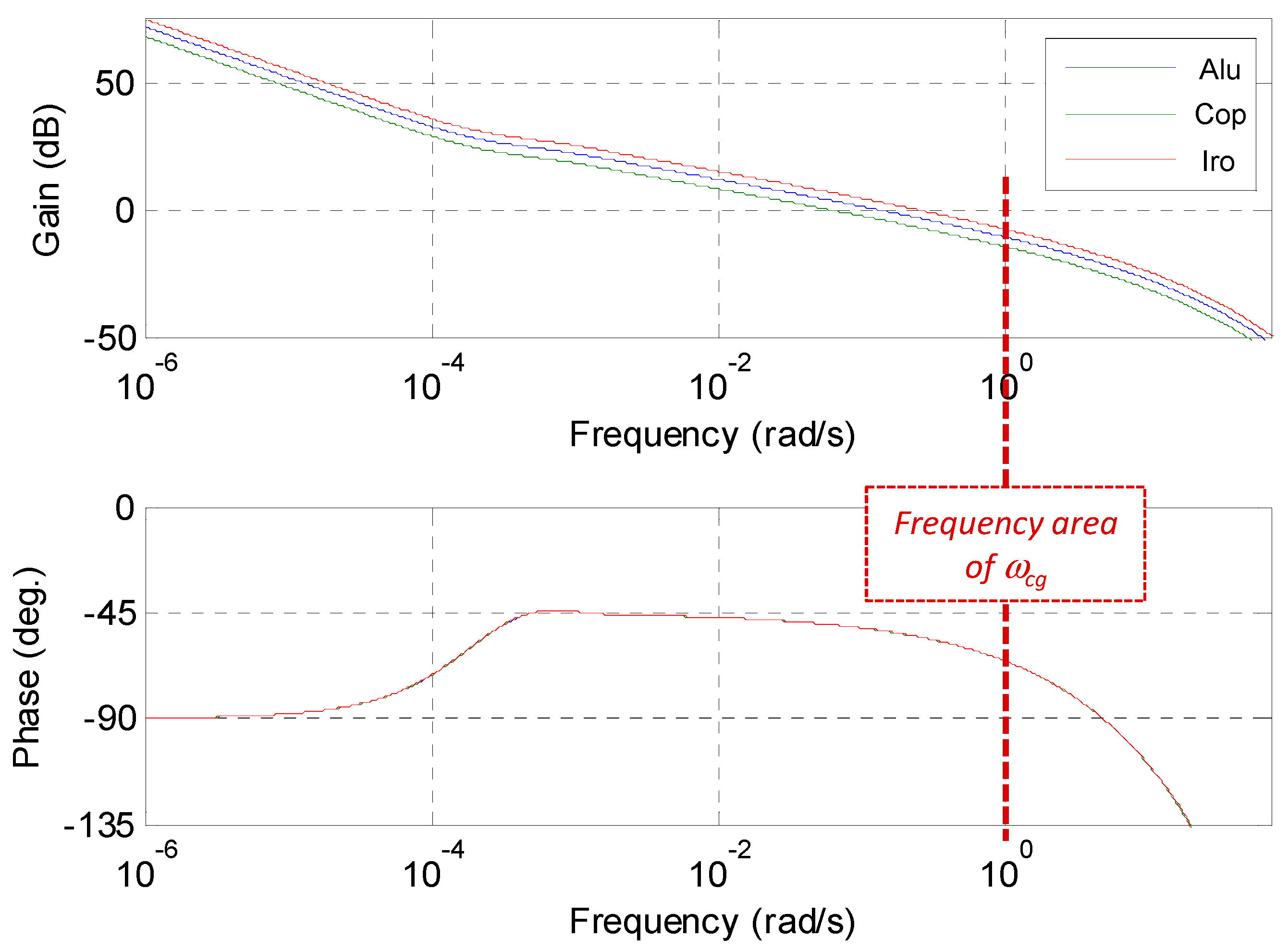
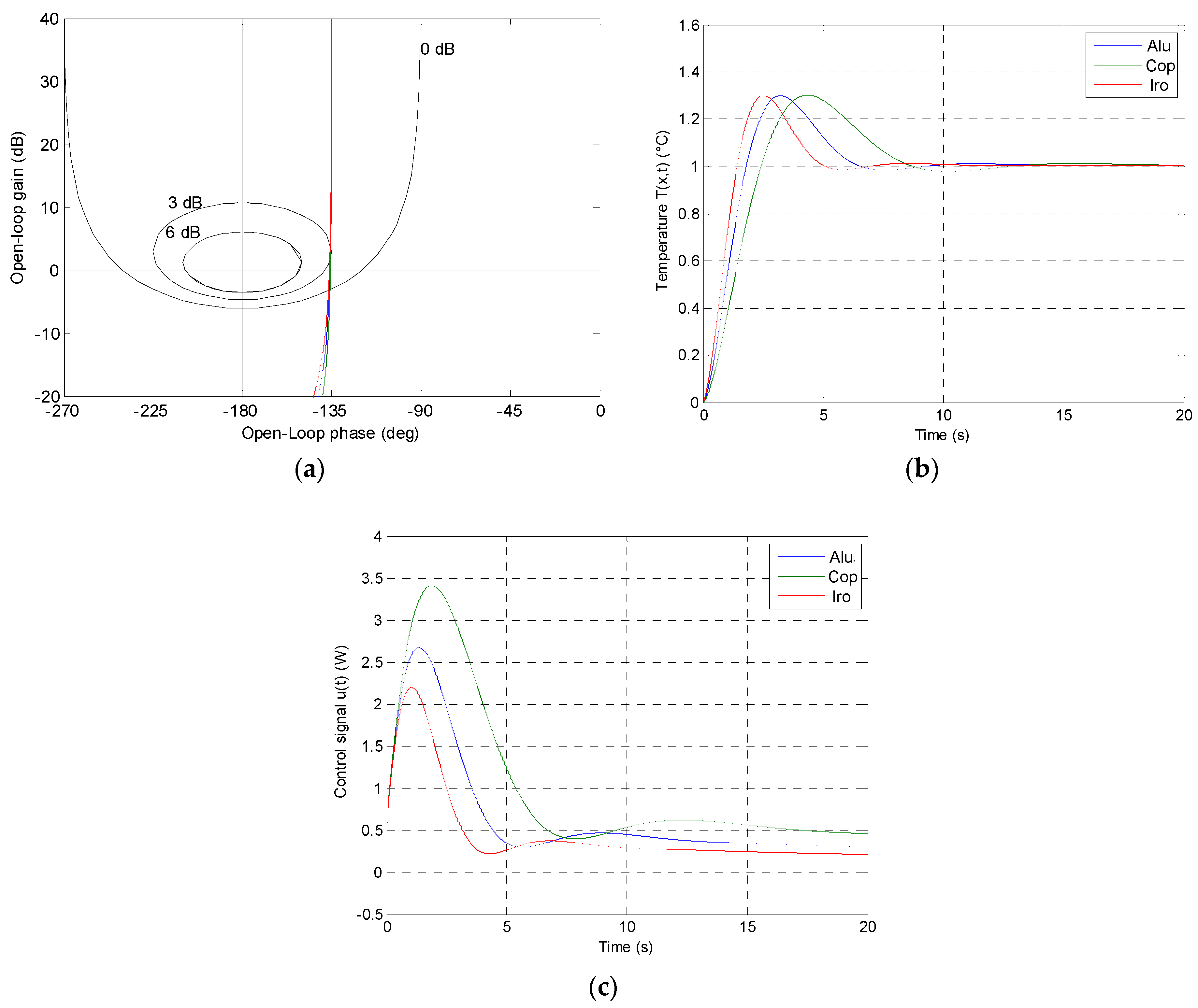
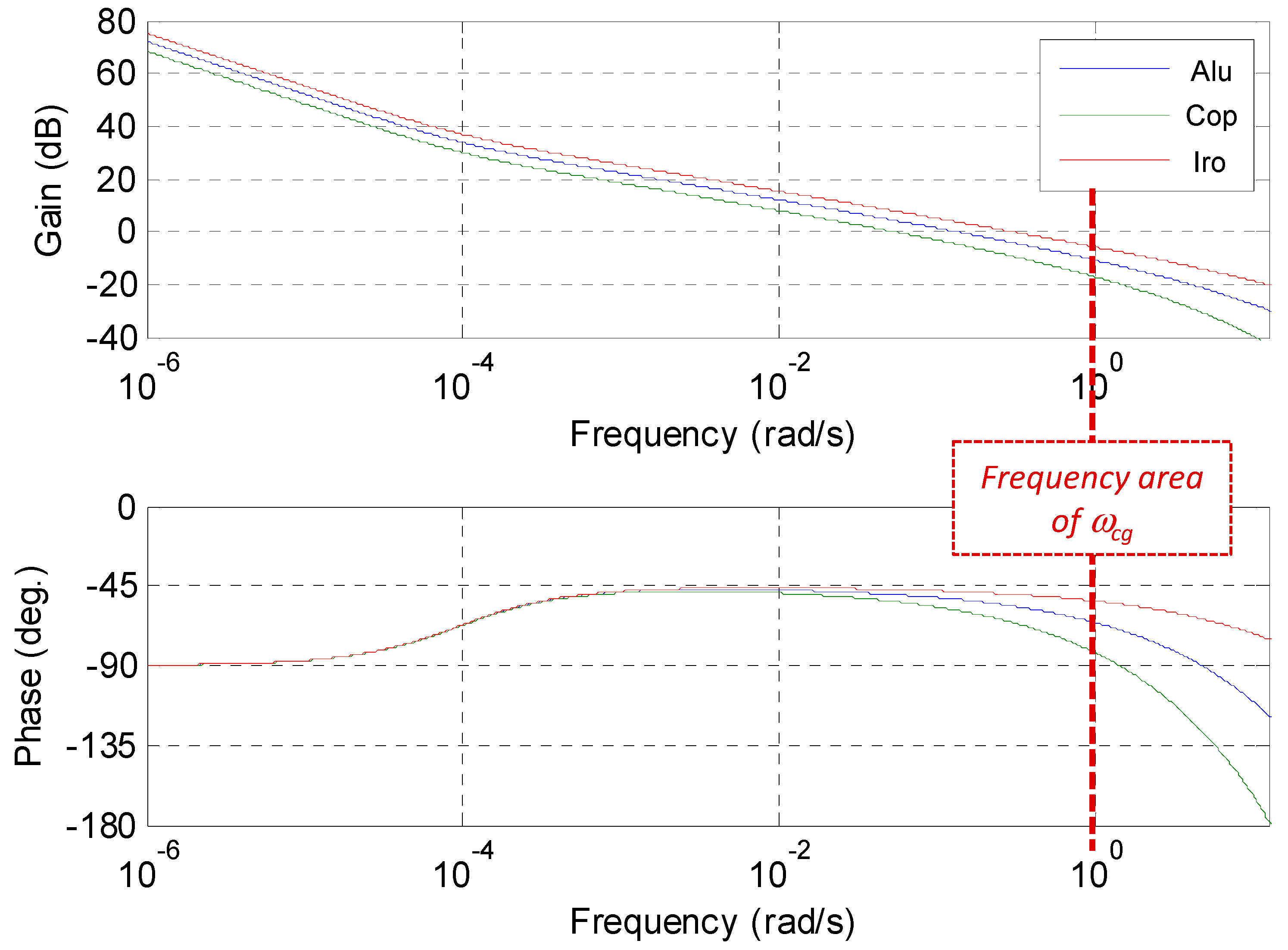
• A crossover frequency ω_cg = 1 rad/s;
• A phase margin M_φ = 3 dB;

To do so, this paper will be divided as follows: in Section 2, the homogeneous finite and rectangular bar will be presented, along with its mathematical modeling and its boundary conditions. In Section 3, the different applied controllers will be introduced; an overview of the three CRONE generations will also be proposed, along with the conditions of application of each generation. In Section 4, the second CRONE generation will be presented along with two case studies: the first one shows an ideal domain of application where the phase is constant and the gain varies whenever plant parameters change. The second case presents both phase and gain variations, and the use of the already synthesized controller appears to be no more robust. Hence, for this second case study, the third generation controller will be introduced in Section 5, and a performance analysis will be presented. At the end, Section 6 will provide a conclusion and some future works to enrich this work.

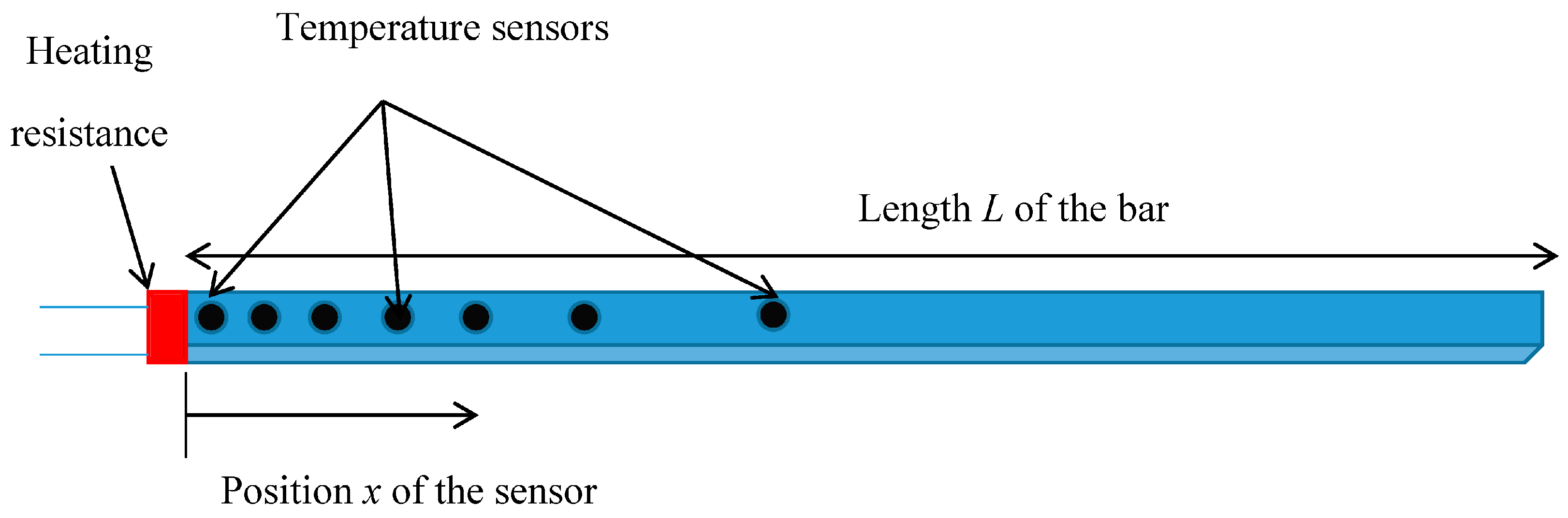
2. Plant Modeling

The homogeneous diffusive interface medium will be presented in this part. The test bench is constituted of a rectangular homogeneous rod with a square section S. It may consist of aluminum, copper, or iron, and it is of a finite distance L, as shown in Figure 1. The characteristics of the medium, its differential equations, and the boundary conditions, along with the features of the material used will be proposed hereafter.

2.1. Partial Differential Equations (PDE)

The input of this medium will be the density of flux ϕ(t) (which is equal to the flux φ(t) divided by the section S of the source), whereas the output is the temperature at a location x. The partial differential equations of this medium are shown in system (1), where the first equation shows the temperature value for any value of x. As for the second equation, it represents the temperature variation at the boundary where the heating element is applied.

$$\{\begin{array}{l}\frac{\partial T\left(x,t\right)}{\partial t}={\alpha }_d\frac{{\partial }^{2}T\left(x,t\right)}{\partial x^2},x>0,t>0\\ -\lambda \frac{\partial T\left(x,t\right)}{\partial x}=\varphi \left(t\right),x=0,t>0\end{array},$$

(1)

where α_d represents the thermal diffusivity of the material, and T(x,t) represents the temperature at the position x for time t.

In the second boundary equation, the flux is not applied, and the temperature along the bar at the initial time (t = 0 s) is expressed by the following system:

$$\{\begin{array}{l}-\lambda \frac{\partial T\left(x,t\right)}{\partial x}=0,x=L,t>0\\ T\left(x,t\right)=0,0\le x<L,t=0\end{array}.$$

(2)

2.2. Plant Transfer Function

Based on the partial differential equations that represent the relation between the applied density of flux ϕ(t) and the temperature variation T(x,t,L) within the diffusive interface medium of length L, one can deduce the transfer function H(x,s,L) that models this system (interested authors can refer to the following references for a detailed calculation of this transfer function [45,46]). Note here that the temperature varies with respect to the material used, the placement x of the temperature sensor, and the length L of the rod. This transfer function H(x,s,L) is given by:

$$\begin{gathered} H\left(x,s,L\right)=\frac{\overline{T}\left(x,s,L\right)}{\overline{\phi }\left(s\right)}=H_0\frac{1}{s^{0.5}}\frac{1}{\tanh \left(\sqrt{\frac{s}{{\omega }_L}}\right)}\frac{\cosh \left(\sqrt{\frac{s}{{\omega }_{Lx}}}\right)}{\cosh \left(\sqrt{\frac{s}{{\omega }_L}}\right)}, \\ {H}_0=\frac{1}{S{\eta }_d},{\eta }_d=\sqrt{\lambda \rho C_p},{\omega }_L=\frac{{\alpha }_d}{L^2},{\omega }_{Lx}=\frac{{\alpha }_d}{{\left(L-x\right)}^2}, \end{gathered}$$

(3)

where $\overline{T}\left(x,s,L\right)$ and $\overline{\varphi }\left(s\right)$ represent the Laplace transform of T(x,t,L) and ϕ(t) respectively, η_d is the thermal effusivity, λ represents the thermal conductivity, ρ is the medium density, and C_p is the medium heat.

From Equation (3), one can notice the fractional order operator ($\sqrt{s}$) residing in the hyperbolical trigonometric functions, as well as the pure semi-integrator. This can confirm, once again, the novelty of this work by applying a fractional order control (the CRONE controller) to, most importantly, a non-integer order plant.

However, the expression of the transfer function H(x,s,L) can be reduced: in fact, as the position of the temperature sensor is neglected with respect to the length of the bar (x << L), one can deduce that ω_Lx ≈ ω_L. Thus, Equation (3) can be written as follows, where this latter defines the validation model of the system:

$$H\left(x,s,L\right)=\frac{\overline{T}\left(x,s,L\right)}{\overline{\varphi }\left(s\right)}=H_0\frac{1}{s^{0.5}}\frac{1}{\tanh \left(\sqrt{\frac{s}{{\omega }_L}}\right)}{e}^{-\sqrt{\frac{s}{{\omega }_x}}},$$

(4)

where ω_x = α_d/x².

2.3. Material Characteristics

As previously proposed, three materials will be used: copper (Cop), iron (Iro), and aluminum (Alu). The last one will be considered for the nominal case.

Table 1. Physical characteristics of the used materials. Alu: aluminum; Cop: copper; Iro: iron.

Material	${\mathit{\alpha }}_{\mathit{d}}$	${\mathit{\eta }}_{\mathit{d}}$	${\mathit{H}}_0$	${\mathit{\varpi }}_{\mathit{L}}$ (rad/s)			${\mathit{\varpi }}_{\mathit{x}}$ (rad/s)
	m2/s	W·K−1·m−2·s0.5	K·s0.5·W−1	L = 0.25 m	L = 0.5 m	L = 1 m	x = 0 cm	x = 0.5 cm	x = 1 cm
Cop.	117 × 10−6	3.72 × 104	0.269	19 × 10−4	4.68 × 10−4	1.17 × 10−4	Infinite	4.68	1.17
Alu.	97 × 10−6	2.41 × 104	0.416	16 × 10−4	3.88 × 10−4	0.97 × 10−4	Infinite	3.88	0.97
Iro.	23 × 10−6	1.67 × 104	0.596	3.68 × 10−4	0.92 × 10−4	0.23 × 10−4	Infinite	0.92	0.23

shows the characteristics of the three materials, along with the values of the two transitional frequencies ω_L and ω_x for three values of the length, L, and the temperature sensor position, x.

When synthesizing the controllers, two case studies will be proposed based on the values of L and x for the three material types. In the next sections, these case studies will be defined in more detail, and the plant uncertainties will be modeled.

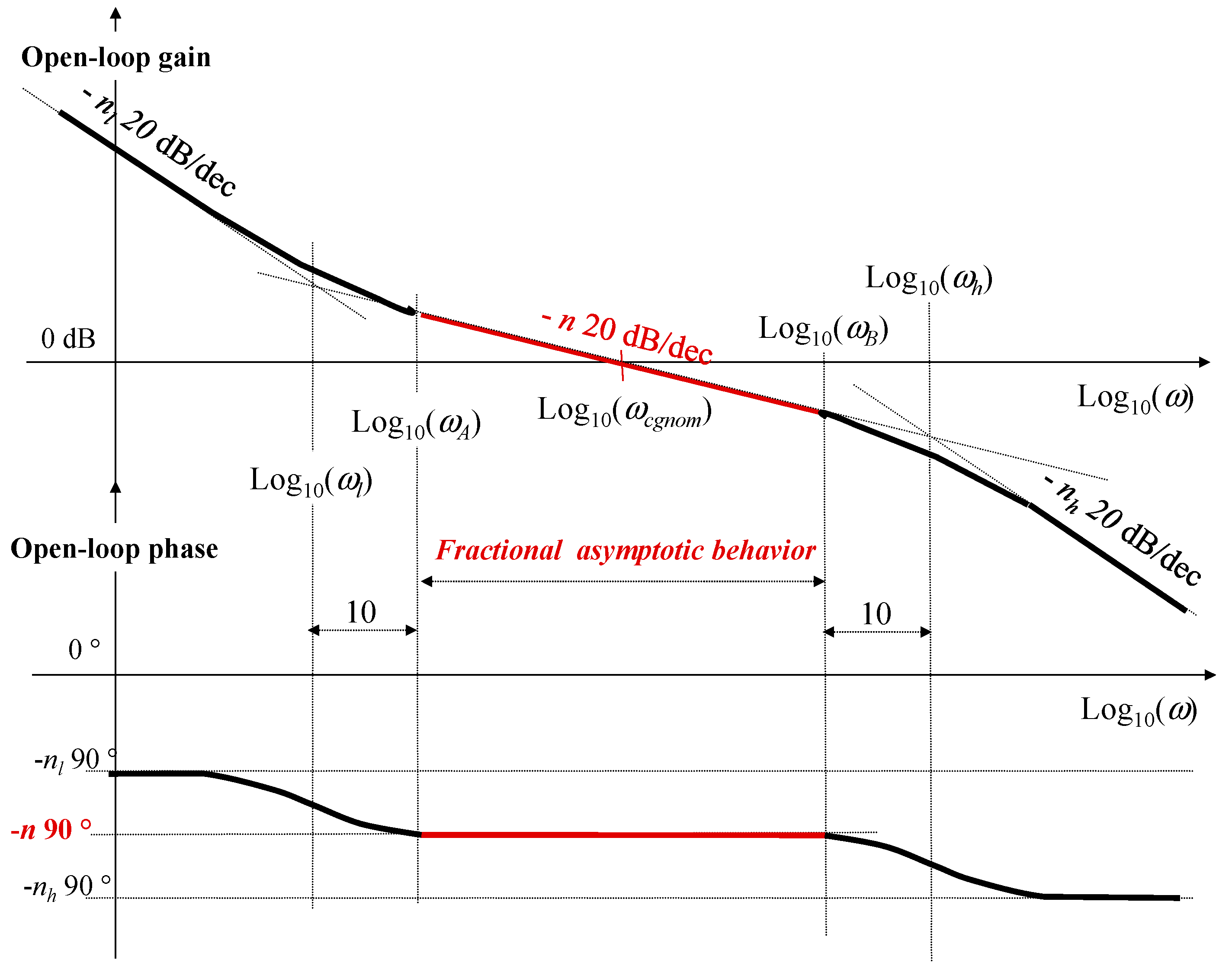
3. CRONE Controllers Presentation

The controllers that would be used in this application are the second and third generation CRONE controllers. In the following, we will present each controller, and the method to synthesize it. The two next sections will show the applications of the second and the third generations using two different case studies. This will help the user understand the conditions in which to apply each of the CRONE generations.

The CRONE controller is the first fractional order controller developed. It was launched in 1975, and it was introduced using three generations. We will focus in this paper on the second and third generations, knowing that the first two generations were treated in previous works [47,48]. However, a brief overview over the three generations will be presented below.

The first generation Crone controller proposes to use a controller without phase variation around crossover frequency ω_cg. Thus, the phase margin variation only results from the plant variation. This strategy has to be used when frequency ω_cg is within a frequency range where the plant phase is constant. In this range, the plant variations are only gain-like. This first generation uses the a priori calculation where the controller transfer function is calculated directly based on the user specifications.

The second generation CRONE control is applied when the plant variations are gain-like around the gain crossover frequency ω_cg, and the plant phase variation is canceled by those of the controller. Thus, there is no phase margin variation when the frequency of ω_cg varies. Such a controller produces a constant open-loop phase whose Nichols locus is a vertical straight line named the frequency template. This controller is synthesized a posteriori, where its transfer function is deduced from the open-loop transfer function.

The third generation Crone controller is used when the plant frequency uncertainty domains are of various types (not only gain-like, but present both gain and phase variation). The vertical template is then replaced by a generalized template or by a multi-template (or curvilinear template) defined by a set of generalized templates. Here also, the transfer function is defined a posteriori based on the open-loop behavior [49].

4. Second CRONE Generation

4.1. Introduction

As the transfer function of this generation is synthesized a posteriori, the transfer function of the open-loop system is defined as follows (for frequencies in the range of [ω_A, ω_B]):

$$\beta (s)={\left(\frac{\omega {}_{cg}}{s}\right)}^n,$$

(5)

where ω_cg is the frequency for which the uncertainties do not lead to any phase variation, n ∈ ℝ and n ∈ [1,2].

The complementary sensitivity function T(s) and the sensitivity function S(s) are defined as follows:

$$T\left(s\right)=\frac{\beta (s)}{1+\beta (s)}=\frac{1}{1+{\left(\frac{s}{\omega {}_{cg}}\right)}^n}\mathrm{and}S\left(s\right)=\frac{1}{1+\beta (s)}=\frac{{\left(\frac{s}{\omega {}_{cg}}\right)}^n}{1+{\left(\frac{s}{\omega {}_{cg}}\right)}^n}.$$

(6)

Around the crossover frequency ω_cg, the Black–Nichols plot of the open-loop transfer function β(s) is a vertical asymptote with a constant phase equal to n, as shown in Figure 2. This asymptote allows having [48]:

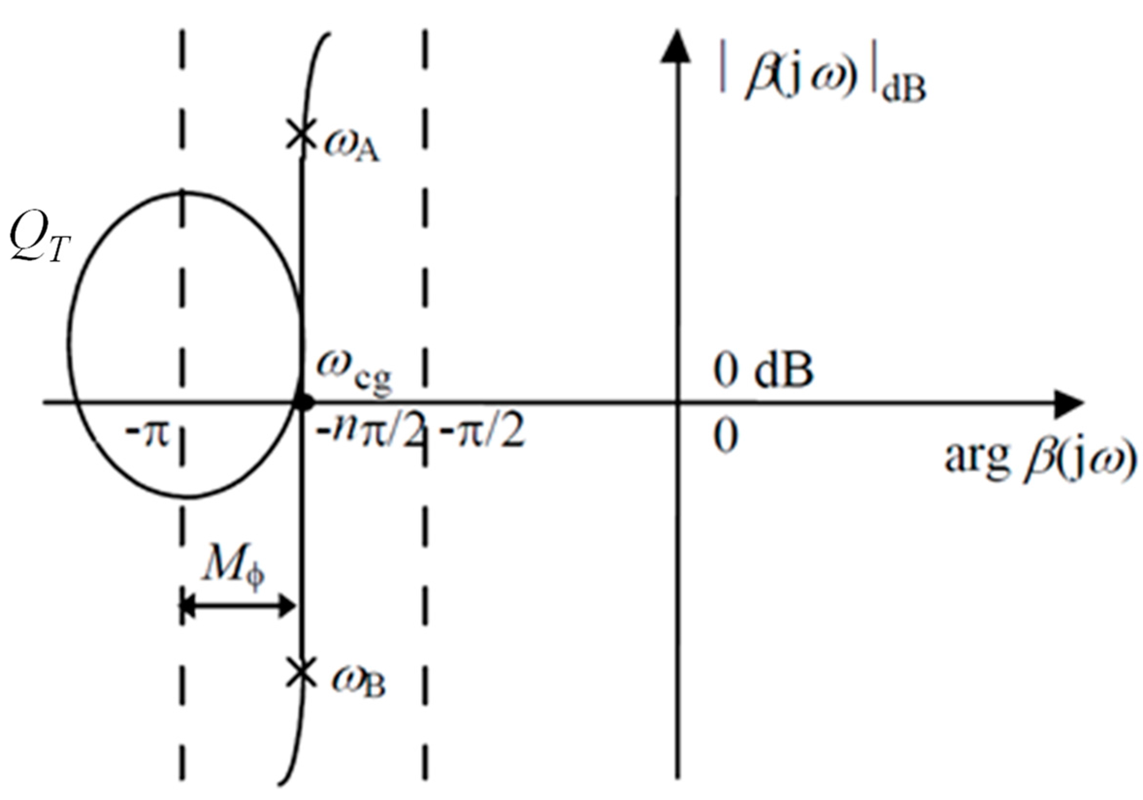
• a robust phase margin M_φ equal to (2−n)×π/2;
• a robust resonance factor Q_T, defined as follows:

  $$Q_T=\frac{\underset{\omega }{\sup }\left|T\left(j\omega \right)\right|}{\left|T\left(j0\right)\right|}=\frac{1}{\sin \left(n\pi /2\right)};$$

  (7)
• a robust gain module M_m, defined as follows:

  $$M_m=\underset{\omega }{\inf }\left|\beta \left(j\omega \right)+1\right|={\left(\underset{\omega }{\sup }\left|S\left(j\omega \right)\right|\right)}^{-1}=\sin \left(n\pi /2\right);$$

  (8)

As for the control signal and the transient error, Equation (5) can be truncated in frequency, and a low pass filter as well as an integrator must be added. Hence, the new form of the open-loop transfer will appear as follows:

$$\beta (s)={\beta }_0{\left(\frac{1+s/\omega {}_l}{s/\omega {}_l}\right)}^{n_l}{\left(\frac{1+s/\omega {}_h}{1+s/\omega {}_l}\right)}^n{\left(1+s/\omega {}_h\right)}^{-n_h},$$

(9)

where ω_l and ω_h represent the low and high transitional frequencies, n is the fractional order (varying between 1 and 2) around the frequency ω_cg, n_l and n_h are the system behavior at low and high frequencies, and β₀ is a constant value that assures a crossover frequency ω_cg. It is expressed in Equation (10):

$${\beta }_0={\left({\omega }_{cg}/\omega {}_l\right)}^{n_l}{\left(1+{\left({\omega }_{cg}/\omega {}_l\right)}^2\right)}^{\left(n-n_l\right)/2}{\left(1+{\left({\omega }_{cg}/\omega {}_h\right)}^2\right)}^{\left(n_h-n\right)/2}.$$

(10)

Figure 3 shows the asymptotic behavior in a Bode diagram for this open-loop transfer function β(s). The fractional order behavior is defined over the interval [ω_A, ω_B], and it belongs to the nominal crossover frequency ω_cgnom. In order to respect the robustness of the stability degree, it is necessary to define the margins for ω_cg, such as:

$$\forall {\omega }_{cg}\in \left[{\omega }_{cg\min };{\omega }_{cg\max }\right],{\omega }_A\le {\omega }_{cg}\le {\omega }_B\Rightarrow \{\begin{array}{l}{\omega }_A\le {\omega }_{cg\min }\hfill \\ {\omega }_B\ge {\omega }_{cg\max }\hfill \end{array}.$$

(11)

As shown in Figure 3, two new cutoff frequencies are introduced (ω_l and ω_h), which help getting the fractional order behavior between ω_A and ω_B. Previous studies have shown that it is sufficient for ω_l to be one decade less ω_B, whereas for ω_l, it must be one decade above ω_h [49].

$$\{\begin{array}{l}{\omega }_l={\omega }_A/10\hfill \\ {\omega }_h=10{\omega }_B\hfill \end{array}.$$

(12)

Thus, one can define ω_cgnom as being the geometric median of ω_l and ω_h. Added to that, a new parameter r, being the ratio of ω_B and ω_A, is introduced:

$$\{\begin{array}{l}\sqrt{{\omega }_l{\omega }_h}={\omega }_{cgnom}\hfill \\ r=\frac{{\omega }_B}{{\omega }_A}\hfill \end{array}.$$

(13)

Αs a consequence, ω_l and ω_h could be written with respect to ω_cgnom and r as follows:

$$\{\begin{array}{l}\sqrt{{\omega }_l{\omega }_h}={\omega }_{cgnom}\hfill \\ \frac{{\omega }_h}{{\omega }_l}=100r\hfill \end{array}\Rightarrow \{\begin{array}{l}{\omega }_l={\omega }_{cgnom}/\left(10\sqrt{r}\right)\hfill \\ {\omega }_h={\omega }_{cgnom}10\sqrt{r}\hfill \end{array}.$$

(14)

Once the open-loop transfer function is calculated, one can conclude the CRONE controller transfer function as being the ratio of the open-loop transfer function β(jω) over the nominal plant’s transfer function P₀(jω):

$$C_F\left(j\omega \right)=\beta (j\omega )/P_0\left(j\omega \right).$$

(15)

A last step is always needed in order to pass from the fractional form C_F(jω) to the rational form C_R(jω). Several methods could be applied in this case; however, one simple method is based on the representation of the function using a recursive distribution of poles and zeros. Each pole and zero form a cell. The higher the number of cells, the most accurate the results are, but the more complex the transfer function would be. However, four to eight cells would be enough, as the fractional frequency range is below three decades [50]. Another option exists in using the CRONE toolbox, which can give the rational representation of the fractional form since it knows the frequency response of C_F(jω) [51,52].

4.2. First Case Study

4.2.1. Plant Parameters

As the objectives of the second generation of the CRONE controller is to have a constant phase with a variable gain when varying the parameters of the plant, the choice of the values of L and x is crucial in order to apply this generation. Hence, these values are listed below:

-

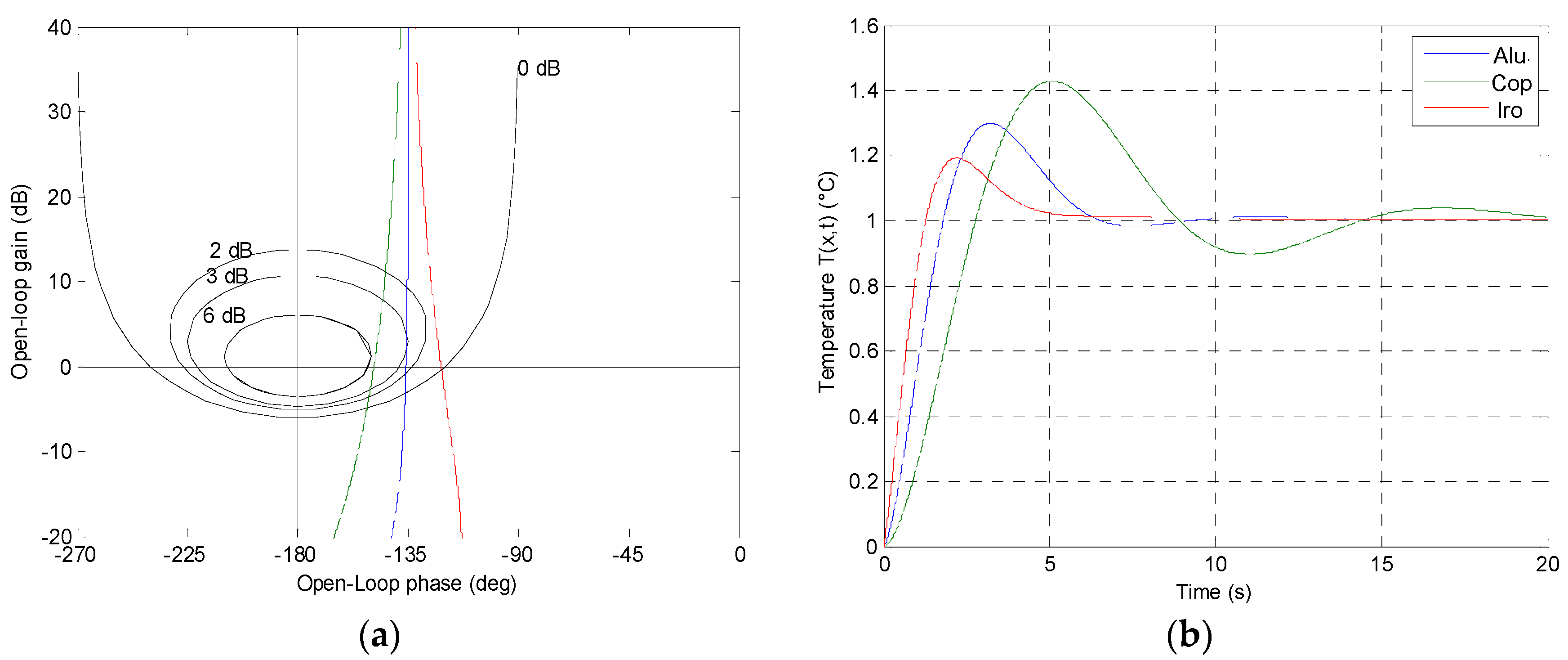
Aluminum, L = 1 m and x = 0.5 cm → ω_L = 0.97 10⁻⁴ rad/s and ω_x = 3.88 rad/s;

-

Copper, L = 1.1 m and x = 0.55 cm  → ω_L = 0.97 10⁻⁴ rad/s and ω_x = 3.87 rad/s;

-

Iron, L = 0.49 m and x = 0.243 cm    → ω_L = 0.96 10⁻⁴ rad/s and ω_x = 3.89 rad/s.

Figure 4 shows the Bode diagrams for the three plants. The phase constancy for the three outputs is well noted; however, the changes in the gain are also observed. Hereafter, the aluminum will be considered the nominal case, whereas the copper and iron will be considered the extreme cases.

4.2.2. Synthesis Model

The plant transfer function H(x,s,L), which was already presented in Equations (3) and (4), could be written in another way in order to facilitate the computation of the controller transfer function. Thus, it could be expressed as follows based on the approximation for the tanh function. The new model P₂(s) in Equation (16) will be considered as the synthesis model that will be easier to use in order to calculate the controller transfer function. Interested readers can refer to a previous work of the authors for more details about the calculations [53].

$$P_2\left(s\right)=H_0^{*}\frac{{\left(1+s/{\omega }_L\right)}^{0.5}}{s/{\omega }_L}{e}^{-\sqrt{\frac{s}{{\omega }_x}}},$$

(16)

where

$$H_0^{*}=\frac{H_0}{{\omega }_L^{0.5}}.$$

(17)

Figure 5 represents the Bode plots of P₂(jω) (in blue) and of H(x,jω,L) (in green) obtained with aluminum for L = 1 m and x = 0.5 cm. It is well noted the coherence of both plots (for the gain and the phase) in the frequency range around ω_cg.

4.2.3. Controller Transfer Function

As already discussed, the synthesis of the CRONE controller transfer function is done a posteriori. Thus, we have first to compute the open-loop transfer function (Equation (9)), then by replacing the plant’s transfer function by its value, we will obtain the controller transfer function, which could be expressed as follows:

$$C_F\left(s\right)={\beta }_0{\left(\frac{1+s/\omega {}_l}{s/\omega {}_l}\right)}^{n_l}{\left(\frac{1+s/\omega {}_h}{1+s/\omega {}_l}\right)}^n\frac{1}{{\left(1+s/\omega {}_h\right)}^{n_h}}\frac{s/{\omega }_L}{H_0^{*}{\left(1+s/{\omega }_L\right)}^{0.5}}{e}^{\sqrt{\frac{s}{{\omega }_x}}}.$$

(18)

Taking into consideration the specifications of the user guide, the different variables can be defined. Thus,

-

n_l = 2, in order to assure a null training error;

-

n_h = 1.5, in order to limit the input sensitivity;

-

Q_T = 3 dB or M_Φ = 45° → n = (180°−M_Φ)/90° = 1.5;

-

ω_cgnom = 1 rad/s ;

So, taking into account the previous values, Equation (18) can be written as follows:

$$C_F\left(s\right)=C_0\left(\frac{\omega {}_l}{s}\right)\frac{{\left(1+s/\omega {}_l\right)}^{2-n}}{{\left(1+s/\omega {}_h\right)}^{1.5-n}{\left(1+s/{\omega }_L\right)}^{0.5}}{e}^{\sqrt{\frac{s}{{\omega }_x}}},$$

(19)

where:

$$C_0=\frac{{\beta }_0{\omega }_l}{H_0^{*}{\omega }_L}.$$

(20)

In order to get rid of the exponent, a Taylor development was needed for e^z when z tends towards zero.

$$\underset{z\to 0}{\lim }{e}_{}^z=1+z+\frac{z^2}{2!}+\frac{z^3}{3!}+\dots +\frac{z^k}{k!}+\dots ={\displaystyle \sum _{k=0}^{\infty }\frac{z^k}{k!}},$$

(21)

When truncated at order 2 and considering that z = (s/ω_x)^0.5, one can obtain:

$$e^{\sqrt{\frac{s}{{\omega }_x}}}\approx 1+{\left(\frac{s}{{\omega }_x}\right)}^{0.5}+\frac{s}{2{\omega }_x}.$$

(22)

So, the fractional approximated form ${\tilde{C}}_F\left(s\right)$ is defined by:

$$\begin{array}{cc}\hfill {\tilde{C}}_F\left(s\right)& =C_0\left(\frac{\omega {}_l}{s}\right)\frac{{\left(1+s/\omega {}_l\right)}^{2-n}}{{\left(1+s/\omega {}_h\right)}^{1.5-n}{\left(1+s/{\omega }_L\right)}^{0.5}}\left(1+{\left(\frac{s}{{\omega }_x}\right)}^{0.5}+\frac{s}{2{\omega }_x}\right)\hfill \\ \hfill & =\frac{C_0^{*}}{s}\left(1+{\left(\frac{s}{{\omega }_x}\right)}^{0.5}+\frac{s}{2{\omega }_x}\right)\hfill \end{array}$$

(23)

where $C_0^{*}=C_0{\omega }_l=2.405\mathrm{W}\cdot {\mathrm{s}}^{-1}\cdot {\mathrm{deg}}^{-1}$, and ω_x = 3.88 rad/s.

Referring to Equation (23), the controller is constituted of a simple integrator, which allows removing the noise caused by the exponent around the crossover frequency ω_cg. For the low frequencies, the controller has an integrator behavior, whereas for high frequencies, it has a proportional behavior.

In order to apply this controller, the rational form is needed. For this example, we will be using the cascade representation, as shown in Equation (24). The use of the CRONE toolbox helps defining the values of the poles and the zeros. The new approximated transfer function will be as follows:

$$C_R\left(s\right)=\frac{C_0^{*}}{s}\frac{{\displaystyle \prod _{j=1}^3\left(1+\frac{s}{{\omega }_{zj}}\right)}}{{\displaystyle \prod _{j=1}^2\left(1+\frac{s}{{\omega }_{pj}}\right)}},$$

(24)

where:

$$\{\begin{array}{ll}{\omega }_{z1}=0.8\mathrm{rad}/\mathrm{s}\hfill & {\omega }_{p1}=1.25\mathrm{rad}/\mathrm{s}\hfill \\ {\omega }_{z2}=6.5\mathrm{rad}/\mathrm{s}\hfill & {\omega }_{p2}=29\mathrm{rad}/\mathrm{s}\hfill \\ {\omega }_{z3}=55\mathrm{rad}/\mathrm{s}\hfill & \hfill \end{array}.$$

(25)

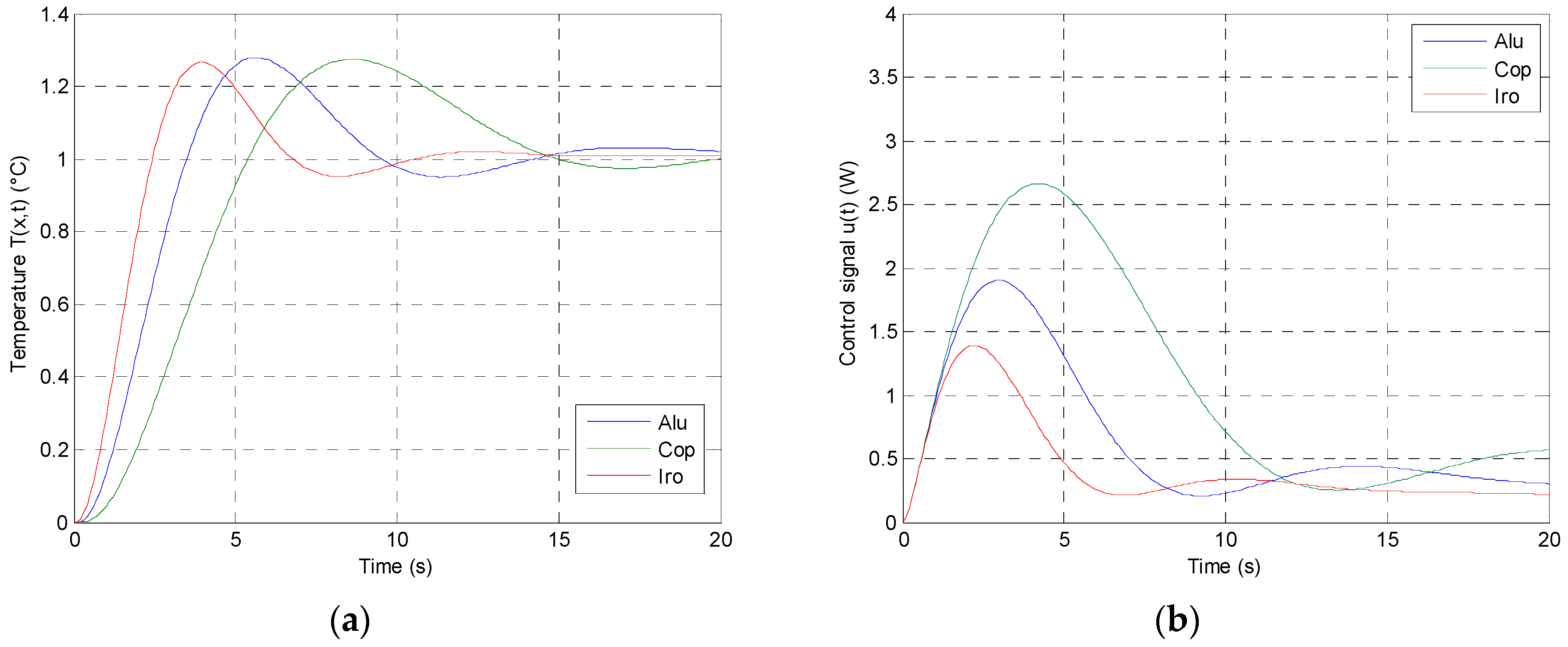
4.2.4. Performance Analysis

Concerning the behavior of the second generation CRONE controller applied to a plant where the uncertainties are modeled only by gain variation and an invariable but non-constant phase for the three plants, the following plots will resume the outcome.

Figure 6 represents the Bode diagrams for the different controllers transfer functions: the fractional form ${\tilde{C}}_F\left(s\right)$ (in blue), and the rational form $C_R\left(s\right)$ (in green).

Figure 7 shows the open-loop Black–Nichols plots (a), the closed-loop step responses (b), and their control inputs for a step input of 1 °C (c) for aluminum (in blue), copper (in green), and iron (in red) for the $C_R\left(s\right)$ controller.

As a conclusion, the exact coherence between the fractional and the rational transfer functions is well noted (Figure 6). Concerning the robustness of the controller, one can see clearly that the three open-loop transfer functions in the Nichols diagram are tangent to the same contour (3 dB). As for the closed-loop step responses, all three outputs have the same first overshoot value and the same damping ratio. Thus, we can confirm that the second generation CRONE controller is robust whenever the conditions of application of this generation are met.

4.3. Second Case Study

In this second case study, we will choose L and x arbitrarily in such a way that the plant will present both phase and gain variations when changing the parameters of the plant, and we will apply the previously synthesized controller (Equations (24) and (25) to study the performance of the new system.

4.3.1. Plant Parameters

The values of L and x chosen for this case study are as follows:

-

Aluminum, L = 1 m and x = 0.5 cm   → ω_L = 0.97 10⁻⁴ rad/s and ω_x = 3.88 rad/s;

-

Copper, L = 1.1 m and x = 1 cm   → ω_L = 0.97 10⁻⁴ rad/s and ω_x = 1.17 rad/s;

-

Iron, L = 0.49 m and x = 0.1 cm    → ω_L = 0.96 10⁻⁴ rad/s and ω_x = 23 rad/s.

Figure 8 shows the Bode diagrams for the three plants. Both the phase and the gain vary when changing the parameters of the plant. As for the first case study, aluminum will be considered as the nominal case, whereas copper and iron will be considered the extreme cases.

4.3.2. Synthesis Model

Based on the exact plant transfer function shown in Equation (4), the synthesis model of the plant for this second case study can be approximated by the following transfer function:

$$P_2\left(s\right)=H_0^{*}\frac{{\left(1+s/{\omega }_L\right)}^{0.5}}{s/{\omega }_L}{e}^{-\sqrt{\frac{s}{{\omega }_x}}},$$

(26)

where the values of $H_0^{*}$, ω_L and ω_x remain unchanged as they were presented for the first case study (refer to Section 4.2.2 and Section 4.2.3).

4.3.3. Controller Transfer Function

As already presented, the controller synthesized for the first case study will be used for this second case, as the nominal plant transfer function (e.g., the aluminum) remains the same. Thus, the controller exact transfer function is the one presented in Equation (23), whereas its rationalized form is shown in Equation (24).

4.3.4. Performance Analysis

Concerning the behavior of the second generation CRONE controller applied to a plant where the uncertainties are modeled by gain and phase variation, the plots of Figure 9 will resume the outcome.

Figure 9 shows the open-loop Black–Nichols plots (a) and the closed-loop step responses (b) for aluminum (in blue), copper (in green) and iron (in red) for the C_R(s) controller.

Concerning the robustness of this controller, one can see clearly that the three open-loop transfer functions in the Nichols diagram are no more tangent to the same contour at 3 dB. As for the closed-loop step responses, the first overshoot value and the damping ratio of the three systems are not constant (we can notice that the first overshoot varies between 19% and 42%). Thus, we can confirm that the second generation CRONE controller is no more robust whenever the conditions of the applied plant are not verified.

However, we will use this second case study to calculate the third generation CRONE controller and analyze its behavior.

5. Third CRONE Generation

5.1. Introduction

The open-loop transfer function, when using the third generation CRONE controller, is defined as being the real part of the fractional complex integrator. It is expressed as follows:

$$\beta (s)={\mathrm{Re}}_{/i}{\left(\frac{{\omega }_{cg}}{s}\right)}^n,$$

(27)

where n = a + ib ∈ C_i and s = +jω ∈ C_j. The real order a determines the phase placement in the Nichols chart, whereas the imaginary part b shows its angle with respect to the vertical axis, as shown in Figure 10.

As we will have an infinite number of asymptotes, the main objective of this CRONE controller will be to optimize the parameters of the open-loop transfer function in a way that includes complex and fractional order integration on a certain frequency range, thus:

$${\beta }_0(s)={\beta }_l(s){\beta }_m(s){\beta }_h(s),$$

(28)

where β_m(s) is the set of models defined within a frequency range, which allows us to write:

$${\beta }_m(s)={{\displaystyle \prod _{k=-N^{-}}^{N^{+}}{C}_k^{\mathrm{sign}\left(b{}_k\right)}\left({\alpha }_k\frac{1+s/{\omega }_{k+1}}{1+s/{\omega }_k}\right)}}^{a_k}{\left({\mathrm{Re}}_{/i}\left\{{\left({\alpha }_k\frac{1+s/{\omega }_{k+1}}{1+s/{\omega }_k}\right)}^{i{b}_k}\right\}\right)}^{-q_k\mathrm{sign}\left(b_k\right)}$$

(29)

where:

$${\alpha }_k={\left(\frac{{\omega }_{k+1}}{{\omega }_k}\right)}^{1/2}\mathrm{for}k\ne 0\mathrm{and}{\alpha }_0={\left(\frac{1+{\left({\omega }_r/{\omega }_0\right)}^2}{1+{\left({\omega }_r/{\omega }_1\right)}^2}\right)}^{1/2}$$

(30)

and:

$${\beta }_l\left(s\right)=C_l{\left(\frac{1+s/{\omega }_{N^{-}}}{s/{\omega }_{N^{-}}}\right)}^{n_l}\mathrm{and}{\beta }_h\left(s\right)=C_h{\left(\frac{s}{{\omega }_{N^{+}}}+1\right)}^{-n_h},$$

(31)

knowing that:

$$\{\begin{array}{l}{N}^{+},N^{-}\mathrm{and}{q}_k{}_{}\in N^{+}\\ {\omega }_r,{\omega }_k,{\omega }_k{{}_{+}}_1,{\alpha }_k,C_k,C_l,C_h,a_k\mathrm{and}{b}_k\in R.\end{array}$$

(32)

As the calculation of all of these parameters is very difficult because of the enormous number of parameters, the CRONE toolbox has been deployed.

5.2. CRONE Toolbox

The main purpose of this toolbox is to calculate the CRONE controller transfer function based on the plant transfer function, as well as the parametric uncertainties of the system. The toolbox can specify which generation is the most suitable to answer the user guide specifications, and it can deliver the controller transfer function in a rational form.

As we are limited in space, interested authors can refer to the following references for more information concerning the toolbox and its characteristics [49,54,55,56].

5.3. Case Study

As already proposed, the second case study, which was proposed for the second CRONE generation, will be treated for this generation. Thus, we will be dealing with a system where both phase and gain are varying over the frequency range.

5.3.1. Plant Parameters

The plant parameters are the ones used for the second case study (refer to Section 4.3. Figure 8 showed the Bode diagram plots for the three plants. Here also, aluminum will be considered the nominal case.

5.3.2. Synthesis Model

In order to synthesize the controller transfer function, the CRONE toolbox was used for the third generation as the computation of the variable is difficult especially that the order is complex and fractional.

Hence, when using the toolbox along with the same user specifications set in the previous controller, the values of the variables of the open-loop transfer function are obtained as follow:

$$\{\begin{array}{ll}{\omega }_0=0.03896\mathrm{rad}/\mathrm{s}\hfill & q_0=6\hfill \\ a_0=1.4927\hfill & C_0=13.217\hfill \\ b_0=-0.6496\hfill & K=34.11\hfill \\ b_0^{\prime }=-0.2379\hfill & {\omega }_1=74.092\mathrm{rad}/\mathrm{s}\hfill \end{array}.$$

(33)

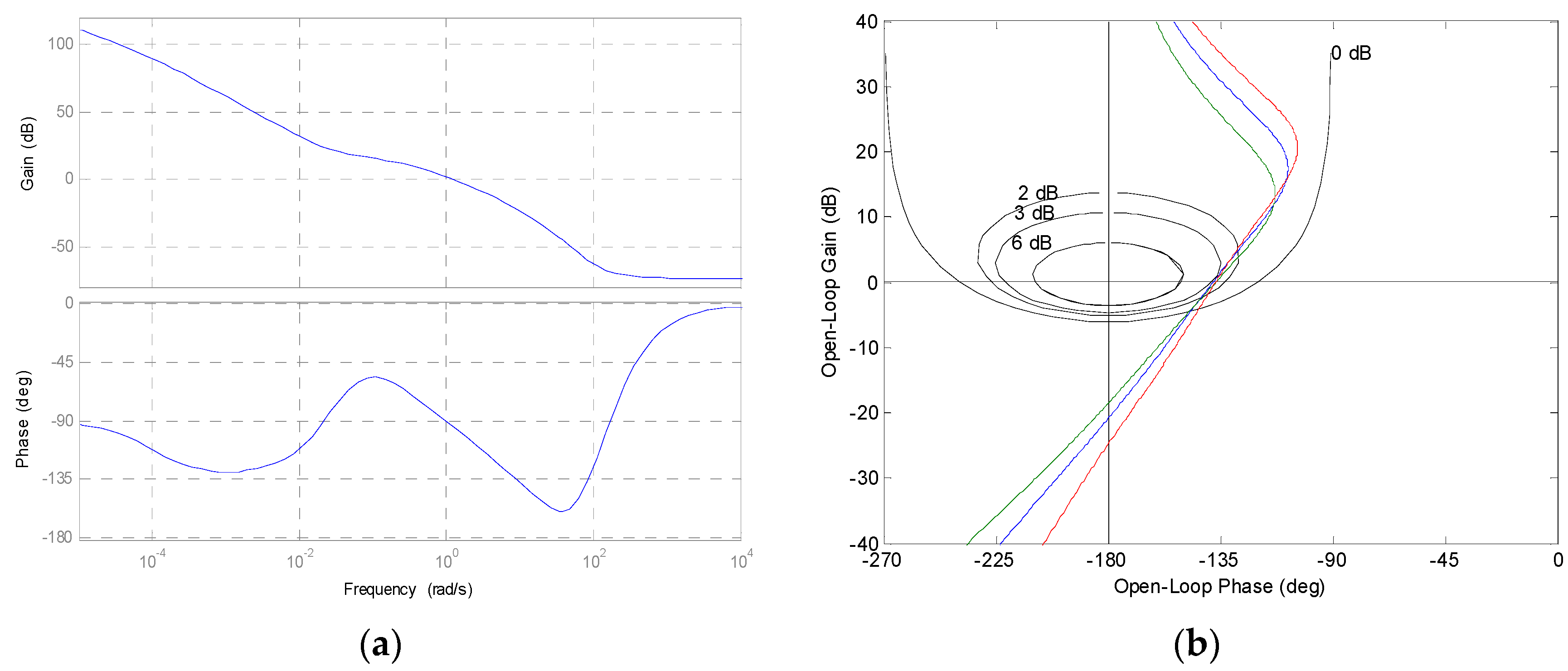
5.3.3. Performance Analysis

Concerning the performance analysis for the third generation CRONE controller, Figure 11 represents the Bode diagrams for the rational controller C_R(s) (a), the Nichols plot of the open loop (b), the Bode gain diagrams for the sensitivity functions S(s) (c) and T(s) (d) (as presented in system (6)), for aluminum (in blue), copper (in green) and iron (in red).

Figure 12 represents the closed step response for the temperature at location x and for time t (a), and the corresponding control signals u(t) (b) for a step input of 1 °C. This will be applied for aluminum (in blue), copper (in green), and iron (in red).

As for the results, Figure 11b shows that the three Nichols plots are tangent to the same contour (3 dB) for a given gain, which may reflect the robustness of the controller. Almost the same results appear when plotting the sensitivity functions where the resonance factor is constant for the three plants (Figure 11c,d). Concerning the time domain responses, it is clear that the three plants have the same first overshoot and the same damping factor, which can prove, once again, the robustness of the third generation CRONE controller.

6. Conclusions and Future Works

As a conclusion, the results show that the second generation CRONE controller is robust when the variations in the plant are modeled with gain changes, whereas the phase remains the same for all of the plants (even if not constant). Nevertheless, the third generation CRONE controller showed a good robustness when changing the parameters of the plant and when encountering both gain and phase variations.

As for the future works, lots of ideas come to mind in order to enrich this study. Below are some of the proposed tasks:

-

Implement this system on a real test bench;

-

Study the accuracy of this system when varying the position of the temperature sensors; this deviation is due involuntarily when implementing the test bench;

-

Apply other regulators to control this fractional order plant as the sliding mode control (with its multiple types), H_inf robust control, and much more;

-

Introduce some estimators to evaluate the temperature value at some location where the temperature sensor can’t be placed.

References

- Vašak, M.; Starčić, A.; Martinčević, A. Model predictive control of heating and cooling in a family house. In Proceedings of the 34th International Convention MIPRO, Opatija, Croatia, 23–27 May 2011. [Google Scholar]
- Van Leeuwen, R.; de Wit, J.; Fink, J.; Smit, G. House thermal model parameter estimation method for Model Predictive Control applications. In Proceedings of the IEEE Eindhoven PowerTech, Eindhoven, The Netherlands, 29 June–2 July 2015. [Google Scholar]
- Mihai, D. Fuzzy control for temperature of the driver seat in a car. In Proceedings of the 2012 International Conference on Applied and Theoretical Electricity (ICATE), Craiova, Romania, 25–27 October 2012. [Google Scholar]
- He, B.; Liang, R.; Wu, J.; Wang, X. A Temperature Controlled System for Car Air Condition Based on Neuro-fuzzy. In Proceedings of the International Conference on Multimedia Information Networking and Security, Wuhan, China, 18–20 November 2009. [Google Scholar]
- Erikson, B. Insulation temperature standards for industrial-control coils. Electr. Eng. 1944, 63, 546–548. [Google Scholar] [CrossRef]
- Jones, B. Thermal Co-ordination of Motors, Control, and Their Branch Circuits on Power Supplies of 600 Volts and Less. Trans. Am. Inst. Electr. Eng. 1942, 61, 483–487. [Google Scholar] [CrossRef]
- Zucker, M. Thermal rating of overhead line wire. Electr. Eng. 1943, 62, 501–507. [Google Scholar] [CrossRef]
- Moore, R. The control of a thermal neutron reactor. Proc. IEE Part II Power Eng. 1953, 100, 197–198. [Google Scholar] [CrossRef]
- Bowen, J.H. Automatic control characteristics of thermal neutron reactors. J. Inst. Electr. Eng. 1953, 100, 122–123. [Google Scholar]
- Fink, L.H. Control of thermal environment of buried cable Systems. Electr. Eng. 1954, 73, 406–412. [Google Scholar] [CrossRef]
- Schmill, J.V. Mathematical Solution to the Problem of the Control or the Thermal Environment or Buried Cables. Trans. Am. Inst. Electr. Eng. Part III Power Appar. Syst. 1960, 79, 175–180. [Google Scholar] [CrossRef]
- Bhuvaneswari, T.; Yao, J.H. Automated greenhouse. In Proceedings of the IEEE International Symposium on Robotics and Manufacturing Automation, Kuala Lumpur, Malaysia, 15–16 December 2014. [Google Scholar]
- Rodríguez-Gracia, D.; Piedra-Fernández, J.; Iribarne, L. Adaptive Domotic System in Green Buildings. In Proceedings of the 4th International Congress on Advanced Applied Informatics, Okayama, Japan, 12–16 July 2015. [Google Scholar]
- Kumar, A. Numerical Modeling of the Thermal Boundary Layer near a Synthetic Crude Oil Plant. J. Air Pollut. Control Assoc. 1979, 29, 827–832. [Google Scholar] [CrossRef] [PubMed]
- Van Schravendijk, B.; de Koning, W.; Nuijen, W. Modeling and control of the wafer temperatures in a diffusion furnace. J. Appl. Phys. 1987, 61, 1620–1627. [Google Scholar] [CrossRef]
- De Waard, H.; de Koning, W. Modeling and control of diffusion and low-pressure chemical vapor deposition furnaces. J. Appl. Phys. 1990, 67, 2264–2271. [Google Scholar] [CrossRef]
- Özişik, M.-N. Heat Conduction; John Wiley & Sons: Ney York, NY, USA, 1980. [Google Scholar]
- Özişik, M.-N. Heat Transfer, a Basic Approach; McGraw-Hill: New York, NY, USA, 1985. [Google Scholar]
- Trigeassou, J.-C.; Poinot, T.; Lin, J.; Oustaloup, A.; Levron, F. Modeling and identification of a non integer order system. In Proceedings of the European Control Conference, Karlsruhe, Germany, 31 August–3 September 1999. [Google Scholar]
- Benchellal, A.; Poinot, T.; Trigeassou, J.-C. Approximation and identification of diffusive interfaces by fractional models. Signal Proc. 2006, 86, 2712–2727. [Google Scholar] [CrossRef]
- Benchellal, A.; Poinot, T.; Trigeassou, J.-C. Fractional Modelling and Identification of a Thermal Process. J. Vib. Control 2008, 14, 1403–1414. [Google Scholar] [CrossRef]
- Battaglia, J.; Cois, O.; Puigsegur, L.; Oustaloup, A. Solving an inverse heat conduction problem using a non-integer identified model. Int. J. Heat Mass Transf. 2001, 44, 2671–2680. [Google Scholar] [CrossRef]
- Battaglia, J.-L.; Maachou, A.; Malti, R.; Melchior, P.; Oustaloup, A. Nonlinear heat diffusion simulation using Volterra series expansion. Int. J. Therm. Sci. 2013, 71, 80–87. [Google Scholar] [CrossRef]
- Maachou, A.; Malti, R.; Melchior, P.; Battaglia, J.-L.; Oustaloup, A.; Hay, B. Application of fractional Volterra series for the identification of thermal diffusion in an ARMCO iron sample subject to large temperature variations. In Proceedings of the 18th IFAC World Congress (IFAC WC’11), Milano, Italy, 28 August–2 September 2011. [Google Scholar]
- Maachou, A.; Malti, R.; Melchior, P.; Battaglia, J.-L.; Oustaloup, A.; Hay, B. Thermal identification using fractional linear models at high temperatures. In Proceedings of the 4th IFAC Workshops on Fractional Differentiation and its Applications (IFAC FDA’10), Badajoz, Spain, 18–20 October 2010. [Google Scholar]
- Malti, R.; Sabatier, J.; Akçay, H. Thermal modeling and identification of an aluminium rod using fractional calculus. In Proceedings of the 15th IFAC Symposium on System Identification, Saint-Malo, France, 6–8 July 2009. [Google Scholar]
- Drapaca, C.; Sivaloganathan, S. A fractional model of continuum mechanics. J. Elast. 2012, 107, 107–123. [Google Scholar] [CrossRef]
- Sumelka, W. Thermoelasticity in the framework of the fractional continuum mechanics. J. Therm. Stress. 2014, 37, 678–706. [Google Scholar] [CrossRef]
- Lazopoulos, K.; Lazopoulos, A. On fractional bending of beams. Arch. Appl. Mech. 2016, 86, 1133–1145. [Google Scholar] [CrossRef]
- Bennett, S. A Brief History of Automatic Control. IEEE Control Syst. 1996, 16, 17–25. [Google Scholar] [CrossRef]
- Bode, H. Network Analysis and Feedback Amplifier Design; D. Van Nostrand. Co.: New York, NY, USA, 1945. [Google Scholar]
- Miller, K.; Ross, B. An Introduction to the Fractional Calculus and Fractional Differential Equations; Wiley: New York, NY, USA, 1993. [Google Scholar]
- Samko, S.; Kilbas, A.; Marichev, O. Fractional Integrals and Derivatives: Theory and Applications; Gordon and Breach: Amesterdam, The Netherlands, 1993. [Google Scholar]
- Oustaloup, A. Etude et Réalisation d’un Systme D’asservissement D’ordre 3/2 de la Fréquence d’un Laser à Colorant Continu; Universitu of Bordeaux: Bordeaux, France, 1975. [Google Scholar]
- Oustaloup, A. La Commande CRONE; Hermes: Paris, France, 1991. [Google Scholar]
- Oustaloup, A. La Dérivation non Entière: Théorie, Synthèse et Applications; Hermes: Paris, France, 1995. [Google Scholar]
- Moreau, X.; Altet, O.; Oustaloup, A. Fractional differentiation: An example of phenomenological interpretation. In Fractional Differentiation and Its Applications; Ubooks Verlag: Neusäß, Germany, 2005; pp. 275–287. [Google Scholar]
- Moreau, X.; Ramus-Serment, C.; Oustaloup, A. Fractional Differentiation in Passive Vibration Control. J. Nonlinear Dyn. 2002, 29, 343–362. [Google Scholar] [CrossRef]
- Ortigueira, M. Introduction to fractional linear systems. Part 1. Continuous-time case. IEE Proc. Vis. Image Signal Process. 2000, 147, 62–70. [Google Scholar] [CrossRef]
- Magin, R.; Ortigueira, M.; Podlubny, I.; Trujillo, J. On the fractional signals and systems. Signal Process. 2011, 91, 350–371. [Google Scholar] [CrossRef]
- Machado, J.-A. Fractional Order Systems. Nonlinear Dyn. 2002, 29, 315–342. [Google Scholar] [CrossRef]
- Ionescu, C.; Machado, J.; de Keyser, R. Modeling of the Lung Impedance Using a Fractional-Order Ladder Network With Constant Phase Elements. IEEE Trans. Biomed. Circuits Syst. 2011, 5, 83–89. [Google Scholar] [CrossRef] [PubMed]
- Ortigueira, M.; Machado, J.-A.; Trujillo, J.; Vinagre, B. Advances in Fractional Signals and Systems. Signal Process. 2011, 91, 350–371. [Google Scholar] [CrossRef]
- Tejado, I.; Vinagre, B.; Torres, D.; Pérez, E. Fractional disturbance observer for vibration suppression of a beam-cart system. In Proceedings of the 10th International Conference on Mechatronic and Embedded Systems and Applications, Senigallia, Italy, 10–12 September 2014. [Google Scholar]
- Assaf, R.; Moreau, X.; Daou, R.A.Z.; Christohpy, F. Analysis of hte Fractional Order System in hte thermal diffusive interface—Part 2: Application to a finite medium. In Proceedings of the 2nd International Conference on Advances in Computational Tools for Engineering Applications, Beirut, Lebanon, 12–15 December 2012. [Google Scholar]
- Assaf, R. Modélisation des Phénomènes de Diffusion Thermique Dans un Milieu fini Homogène en vue de L’analyse, de la Synthèse et de la Validation de Commandes Robustes. Ph.D. Thsis, Université de Bordeaux, Bordeaux, France, 2015. [Google Scholar]
- Christophy, F.; Moreau, X.; Assaf, R.; Daou, R.A.Z. Temperature Control of a Semi Infinite Diffusive Interface Medium Using the CRONE Controller. In Proceedings of the 3rd International Conference on Control, Decision and Information Technologies (CoDIT’16), St. Julian’s, Malta, 6–8 April 2016. [Google Scholar]
- Daou, R.A.Z.; Moreau, X.; Christophy, F. Temperature Control of a finite Diffusive Interface Medium Applying CRONE Second Generation. In Proceedings of the 3rd International Conference on Advances in Computational Tools for Engineering Applications, Beirut, Lebanon, 13–15 July 2016. [Google Scholar]
- Lanusse, P.; Malti, R.; Melchior, P. CRONE control system design toolbox for the control engineering community: Tutorial and case study. Philos. Trans. R. Soc. 2013, 371, 20120149. [Google Scholar] [CrossRef] [PubMed]
- Oustaloup, A. Systèmes Asservis Linéaires d’Ordre Fractionnaire; Masson: Paris, France, 1983. [Google Scholar]
- Oustaloup, A. La Dérivation d’Ordre Non Entier; Hermes: Paris, France, 1995. [Google Scholar]
- CRONE Group. CRONE Control Design Modul; Bordeaux University: Bordeaux, France, 2005. [Google Scholar]
- Daou, R.A.Z.; Moreau, X.; Christophy, F. Temperature control of a finite diffusive interface medium using the third generation CRONE controller. In Proceedings of the 20th IFAC World Congress Program, Toulouse, France, 9–14 July 2017. [Google Scholar]
- Lanusse, P.; Nelson-Gruel, D.; Lamara, A. Toward a CRONE toolbox for the design of full MIMO controllers. In Proceedings of the 7th International Conference on Fractional Differentiation and Its Applications (IFAC-IEEE-ICFDA’16), Novi Sad, Serbia, 18–20 July 2016. [Google Scholar]
- Oustaloup, A.; Melchior, P.; Lanusse, P.; Cois, O.; Dancla, F. The CRONE toolbox for Matlab. In Proceedings of the IEEE International Symposium on Computer-Aided Control System Design, Anchorage, AK, USA, 25–27 September 2000. [Google Scholar]
- Malti, R.; Melchior, P.; Lanusse, P.; Oustaloup, A. Towards an object oriented CRONE toolbox for fractional differential systems. In Proceedings of the 18th IFAC World Congress, Milano, Italy, 28 August–2 September 2011. [Google Scholar]