Analytical Solutions to Fractional Fluid Flow and Oscillatory Process Models

Abstract

In this paper, we provide solutions to the general fractional Caputo-type differential equation models for the dynamics of a sphere immersed in an incompressible viscous fluid and oscillatory process with fractional damping using Laplace transform method. We study the effects of fixing one of the fractional indices while varying the other as particular examples. We conclude this article by explaining the dynamics of the solutions of the models.

1. Introduction

The field of fractional calculus has gained increased popularity among researchers lately due its robust and precise modelling of problems that integer order calculus cannot handle. There are many applications of fractional differential equations in diverse fields of studies in recent time, despite the long aged contributions of Niels Henrik Abel in 1823 who was considered the “father of the complete fractional-order calculus framework” [1]. Fractional differential equations have been applied for modelling problems that are related to anomalous diffusion in the oil drilling sector [2], tilt control in rail vehicles [3], romantic and interpersonal relationships [4], and in financial economics [5]. A few months ago, a fractional epidemiological model was applied to improve the defensive strategies of computers to viruses involving Caputo–Fabrizio derivative [6]. The fractional models elicit interesting behaviour and appropriateness over the integer order derivative models. Further applications of fractional calculus in stochastic modelling, physics, dynamics of earthquakes, networking, optics and signal processing, food sciences and in applied mathematics can be found here [7,8,9,10].

Several methods have been proposed and applied to solving differential equations with fractional order in the literature. Each method has its strengths and weaknesses depending on the nature of the model concerned. These methods ranges from reduction to volterra equations [11], compositional method [12], numerical methods [13], series method [14], Mellin, Fourier, Laplace and a combination of these transforms [15,16,17,18]. The Laplace transform method has been widely used to solve constant-coefficient initial value ordinary differential equations because of its robustness in transforming differential equations to algebraic equations, which then translate to the solutions of the original equations when the inverse Laplace transform is taken. Laplace transform method as a hybrid with homotopy analysis technique and homotopy polynomials has been applied to Fitzhugh–Nagumo equation emernating from nerve impulses and the Jeffery–Hamel flow equations in the respective papers [19,20].

In this work, we use the Laplace transform to solve the following general fractional Caputo-type differential model:

$${}_0^c{D}_t^{\alpha }y\left(t\right)+{\mu }_0^c{D}_t^{\beta }y\left(t\right)+\lambda y\left(t\right)=f\left(t\right),$$

(1)

for the dynamics of a sphere immersed in an incompressible viscous fluid $(0<\beta <\alpha <1)$ and for the oscillatory process with fractional damping $(1<\beta <\alpha <2).$ The first fractional derivative in Equation (1) represents a generalization of the ordinary integer order derivative in the classical relaxation-oscillatory process while the second fractional derivative is a generalization of the damping term with positive constant coefficient $\mu .$ This generalization was motivated by the property of history dependence of the fractional derivatives which represents a true description of the relaxation-oscillatory process. In the case of a sphere immersed in an incompressible viscous fluid $(0<\beta <\alpha <1),y\left(t\right)$ is the velocity of the sphere and it is the displacement of the body in the case the oscillatory process with fractional damping $(1<\beta <\alpha <2)$. $\lambda$ is positive constant (which depends on the radius of the sphere), and $f\left(t\right)$ is an external force term. The dynamics of a sphere immersed in an incompressible viscous fluid is a classical problem with numerous applications in engineering and a particular example is the study of a sphere immersed in a viscous fluid under the effect of gravity as modelled by Equation (1). The generalization of the classical relaxation-oscillatory process using fractional derivative was introduced and investigated in [21]. Meanwhile, the problem was solved without introducing neither damping force nor external force term. These two important quantities have been incorporated in this article and solved using Laplace method with an easy to comprehend approach. We also studied the effects of varying one the fractional indices while the other is fixed using the plot function of Matlab R2014b (MathWorks, Natick, MA, USA).

The structure of this paper is as follows: In Section 2, we recall some basic definitions and properties of the fractional calculus. In Section 3, we present the full problems and give their solutions using Laplace transform method. In Section 4, we study the effects of fixing one of the fractional indices while varying the other using some particular examples. The conclusion is given in Section 5.

2. Preliminaries

In this section, we give some preliminary definitions that will be used later on in this article. There are various definitions of fractional integration and derivatives. The widely used definition of a fractional integration is the Riemann–Liouville definition and that of a fractional derivative is the Caputo definition. Perhaps due to some similarities with the integer order differential operators.

Definition 1

(Riemann–Liouville Integral, [22]). Let $f\left(t\right)\in L^1(a,b):=\{f:{\int }_a^b\left|f\left(t\right)\right|dt<\infty \},$ the integrals

$$\begin{array}{c}\hfill {}_a{I}_t^{\alpha }f\left(t\right):=\frac{1}{\Gamma \left(\alpha \right)}{\int }_a^t{(t-s)}^{\alpha -1}f\left(s\right)ds,t>a,\alpha >0.\end{array}$$

(2)

$$\begin{array}{c}\hfill {}_t{I}_b^{\alpha }f\left(t\right):=\frac{1}{\Gamma \left(\alpha \right)}{\int }_t^b{(s-t)}^{\alpha -1}f\left(s\right)ds,t<b,\alpha >0.\end{array}$$

(3)

are called the left-sided and the right-sided Riemann–Liouville fractional integral of order α of the function f respectively.

Definition 2

(Caputo Derivative, [22]). For $\alpha >0,$ the expression

$$\begin{array}{c}\hfill {}_a^c{D}_t^{\alpha }f\left(t\right):=\{\begin{array}{c}{}_a{I}_t^{n-\alpha }{}_a{D}_t^{n}f\left(t\right),n-1<\alpha <n,\\ {}_a{D}_t^{n}f\left(t\right),\alpha =n.\end{array}\end{array}$$

(4)

$${}_a^c{D}_t^{\alpha }f\left(t\right):={(-1)}^n{}_a{I}_t^{n-\alpha }{}_a{D}_t^{n}f\left(t\right),n-1<\alpha <n,$$

(5)

are the left-sided and right-sided Caputo derivatives of order α respectively, provided $f\left(t\right)$ is $n$-times continuously differentiable function.

Basic Properties of the Caputo Fractional Derivative

It is noteworthy to mention the following basic properties of the Caputo fractional derivative.

• ${}_a^c{D}_t^{\alpha }constant=0.$
• ${}_a^c{D}_t^{\alpha }{(t-a)}^k=0,k=0,1,2,\dots ,n-1.$
• ${}_a^c{D}_t^{\alpha }{(t-a)}^{\beta }=\frac{\Gamma (\beta +1)}{\Gamma (\beta -\alpha +1)}{(t-a)}^{\beta -\alpha },\beta >n-1.$
• $\mathcal{L}{\{}_0^c{D}_t^{\alpha }f\left(t\right)\}=s^{\alpha }F\left(s\right)-{\displaystyle \sum _{k=0}^{n-1}}{s}^{\alpha -k-1}{D}^{k}f\left(0\right).$

Definition 3

(Mittag-Lefler Function, [22]).

$$E_{\alpha }\left(z\right)=\sum _{k=0}^{\infty }\frac{z^k}{\Gamma (\alpha k+1)},\alpha \in \mathcal{C},Re\left(\alpha \right)>0,z\in \mathcal{C}.$$

(6)

Equation (6) is called a one-parameter Mittag-Leffler function, otherwise known as, the classical Mittag-Leffler function.

A two-parameter Mittag-Leffler function is a generalization of Equation (6) as defined in [23] is given by the following series expansion

$$E_{\alpha ,\beta }\left(z\right)=\sum _{k=0}^{\infty }\frac{z^k}{\Gamma (\alpha k+\beta )},\alpha ,\beta \in \mathcal{C},Re\left(\alpha \right)>0,Re\left(\beta \right)>0,z\in \mathcal{C}.$$

(7)

We are interested in the Laplace transform of Mittag-Leffler function in the form

$$\mathcal{L}\left\{t^{\beta -1}{E}_{\alpha ,\beta }\left(\lambda t^{\alpha }\right)\right\}=\frac{s^{\alpha -\beta }}{s^{\alpha }-\lambda },Res>0,\left|\lambda s^{-\alpha }\right|<1.$$

(8)

We included a few lines on the Mittag-Lefler function and its Laplace tranform as it motivates the definition of the Wright function and for more details on the Mittag-Lefler function and its calculus one can see [24,25].

Another important function to be used later on is the Wright function, $W_{\alpha ,\beta }\left(z\right).$ It is defined as follows:

Definition 4

(Wright Function, [8]).

$$W_{\alpha ,\beta }\left(z\right)=\sum _{k=0}^{\infty }\frac{z^k}{k!\Gamma (\alpha k+\beta )},\alpha >-1,\beta \in \mathcal{C}.$$

(9)

Equation (9) is usually called the simplest Wright function. This series is absolutely convergent for all $z\in \mathcal{C}$ provided that $\alpha >-1.$ Further, for $\alpha =-1$ it is absolutely convergent for $\left|z\right|<1.$ The more general Wright function is defined as follows:

$${}_1{\Psi }_1\left[\begin{array}{ccc}(n+1,1)& |& -\mu t^{\alpha -\beta }\\ (\alpha n+1,\alpha -\beta )& |\end{array}\right]:=\sum _{j=0}^{\infty }\frac{\Gamma (n+j+1)}{\Gamma (\alpha n+\beta +\alpha j)}\frac{z^j}{j!}.$$

(10)

The Wright function was introduced and investigated by the eminent British mathematician Wright in [26]. This infinite series is convergent in the whole $z$-plane and its asymptotic behaviours have been studied extensively using the method of steepest decent in [27,28]. It has been widely used in the asymptotic theory of partitions, in the Mikusinski operational calculus and in the theory of integral transforms of the Hankel type. Recently, Wright function has appeared in the solution of partial differential equations of fractional order, it was found that the corresponding Green functions can be represented in terms of the Wright function [29,30]. Further extensive discussion on the properties and applications of Wright function can be found in [29]. Further, a generalization of Equation (8) is the three parameter Mittag-Leffler function in [8] defined for complex $z\in \mathcal{C}$ as follows:

$$E_{\alpha ,\beta }^{\rho }\left(z\right):=\sum _{k=0}^{\infty }\frac{{\left(\rho \right)}_k}{\Gamma (\alpha k+\beta )}\frac{z^k}{k!}=\frac{1}{\Gamma \left(\rho \right)}{}_1{\Psi }_1\left[\begin{array}{ccc}(\rho ,1)& |& z\\ (\beta ,\alpha )& |\end{array}\right],\alpha ,\beta \in \mathcal{C},Re\left(\alpha \right)>0,Re\left(\beta \right)>0.$$

(11)

The convergence of the three parameter Mittag-Leffler function was shown in [31,32] and its asymptotic behaviours can be found in [33,34,35]. Further, it is of interest in this present article, the Laplace transform of the Wright function, given by:

$$\mathcal{L}\left(t^{\alpha n}{}_1{\Psi }_1\left[\begin{array}{ccc}(n+1,1)& |& -\mu t^{\alpha -\beta }\\ (\alpha n+1,\alpha -\beta )& |\end{array}\right]\right)=n!\frac{s^{(\alpha -\beta )-(n\beta +1)}}{{\left(s^{\alpha -\beta }+\mu \right)}^{n+1}}.$$

3. Main Results

In this section, we present the main results of this article. We provide the full models including some initial data and prove the general solutions.

3.1. Dynamics of a Sphere Immersed in an Incompressible Viscous Fluid

Consider the first model problem

$${}_0^c{D}_t^{\alpha }y\left(t\right)+{\mu }_0^c{D}_t^{\beta }y\left(t\right)+\lambda y=f\left(t\right),\mu >0,0<\beta <\alpha <1.$$

(12)

subject to the following initial condition:

$$y\left(0\right)=d.$$

(13)

for the dynamics of a sphere immersed in an incompressible viscous fluid. Equation (13) represents the initial velocity at the time $t=0.$

Theorem 1.

The solution of Equation (12) with the condition (13) is given by:

$$\begin{gathered} y\left(t\right)=d\sum _{n=0}^{\infty }{(-\lambda )}^n\frac{t^{\alpha n}}{n!}{}_1{\Psi }_1\left[\begin{array}{ccc}(n+1,1)& |& -\mu t^{\alpha -\beta }\\ (\alpha n+1,\alpha -\beta )& |\end{array}\right] \\ +\mu d\sum _{n=0}^{\infty }\frac{{(-\lambda )}^n}{n!}{t}^{\alpha n+\alpha -\beta }{}_1{\Psi }_1\left[\begin{array}{ccc}(n+1,1)& |& -\mu t^{\alpha -\beta }\\ (\alpha n+\alpha +1-\beta ,\alpha -\beta )& |\end{array}\right] \\ +\left(\sum _{n=0}^{\infty }{(-\lambda )}^n\frac{t^{(n+1)\alpha -1}}{n!}{}_1{\Psi }_1\left[\begin{array}{ccc}(n+1,1)& |& -\mu t^{\alpha -\beta }\\ \left(\right(n+1)\alpha ,\alpha -\beta )& |\end{array}\right]\right)\times F\left(t\right). \end{gathered}$$

Proof. 

By taking the Laplace transform of Equation (12), we have

$$Y\left(s\right)=d\frac{s^{\alpha -1}}{s^{\alpha }+\mu s^{\beta }+\lambda }+\mu d\frac{s^{\beta -1}}{s^{\alpha }+\mu s^{\beta }+\lambda }+\frac{F\left(s\right)}{s^{\alpha }+\mu s^{\beta }+\lambda }$$

(14)

Observe that

$$\begin{gathered} \frac{1}{s^{\alpha }+\mu s^{\beta }+\lambda }=\frac{s^{-\beta }}{s^{\alpha -\beta }+\mu }\frac{1}{\left[1-\left(\frac{-\lambda s^{-\beta }}{s^{\alpha -\beta }+\mu }\right)\right]}, \\ \left|\frac{\lambda s^{-\beta }}{s^{\alpha -\beta }+\mu }\right|<1 \end{gathered}$$

Recall that

$$\begin{gathered} {(1-z)}^{-n}=\sum _{r=0}^{\infty }\left(\genfrac{}{}{0pt}{}{n+r-1}{r}\right)z^r \\ \Rightarrow \frac{1}{s^{\alpha }+\mu s^{\beta }+\lambda }=\sum _{n=0}^{\infty }{(-\lambda )}^n\frac{s^{-\beta -n\beta }}{{\left(s^{\alpha -\beta }+\mu \right)}^{n+1}} \\ =\sum _{n=0}^{\infty }{(-\lambda )}^n\frac{s^{-\beta -n\beta -(n+1)(\alpha -\beta )}}{{\left(1+\mu s^{\beta -\alpha }\right)}^{n+1}} \\ =\sum _{n=0}^{\infty }{(-\lambda )}^n{s}^{-(n+1)\alpha }\sum _{r=0}^{\infty }\left(\genfrac{}{}{0pt}{}{n+r}{r}\right){(-\mu s^{\beta -\alpha })}^r \\ =\sum _{n=0}^{\infty }{(-\lambda )}^n\sum _{r=0}^{\infty }\frac{(n+r)!}{n!r!}{(-\mu )}^r{s}^{-(n+1)\alpha +{(\beta -\alpha )}^r} \end{gathered}$$

Hence from Equation (14), we have

$$\begin{gathered} Y\left(s\right)=d\sum _{n=0}^{\infty }{(-\lambda )}^n\sum _{r=0}^{\infty }\frac{(n+r)!}{n!r!}{(-\mu )}^r{s}^{-n\alpha +(\beta -\alpha )r-1} \\ +\mu d\sum _{n=0}^{\infty }{(-\lambda )}^n\sum _{r=0}^{\infty }\frac{(n+r)!}{n!r!}{(-\mu )}^r{s}^{-(n+1)\alpha +(\beta -\alpha )r+\beta -1} \\ +F\left(s\right)\sum _{n=0}^{\infty }{(-\lambda )}^n\sum _{r=0}^{\infty }\frac{(n+r)!}{n!r!}{(-\mu )}^r{s}^{-(n+1)\alpha +(\beta -\alpha )r} \end{gathered}$$

On taking the inverse Laplace transform we have

$$\begin{gathered} y\left(t\right)=d\sum _{n=0}^{\infty }\frac{{(-\lambda )}^n}{n!}{t}^{n\alpha }\sum _{r=0}^{\infty }\frac{(n+r)!}{r!}{(-\mu )}^r\frac{t^{(\alpha -\beta )r}}{\Gamma [n\alpha +1+(\alpha -\beta \left)r\right]} \\ +\mu d\sum _{n=0}^{\infty }\frac{{(-\lambda )}^n}{n!}{t}^{n\alpha }\sum _{r=0}^{\infty }\frac{(n+r)!}{r!}{(-\mu )}^r\frac{t^{(1+r)(\alpha -\beta )}}{\Gamma \left[\right(n+1)\alpha +(\alpha -\beta )r-\beta +1]} \\ +\left(\sum _{n=0}^{\infty }\frac{{(-\lambda )}^n}{n!}{t}^{n\alpha }\sum _{r=0}^{\infty }\frac{(n+r)!}{r!}{(-\mu )}^r\frac{t^{(\alpha -1)+(\alpha -\beta )r}}{\Gamma \left[\right(n+1)\alpha +(\alpha -\beta \left)r\right]}\right)\times F\left(t\right) \\ \therefore y\left(t\right)=d\sum _{n=0}^{\infty }{(-\lambda )}^n\frac{t^{\alpha n}}{n!}{}_1{\Psi }_1\left[\begin{array}{ccc}(n+1,1)& |& -\mu t^{\alpha -\beta }\\ (\alpha n+1,\alpha -\beta )& |\end{array}\right] \\ +\mu d\sum _{n=0}^{\infty }\frac{{(-\lambda )}^n}{n!}{t}^{\alpha n+\alpha -\beta }{}_1{\Psi }_1\left[\begin{array}{ccc}(n+1,1)& |& -\mu t^{\alpha -\beta }\\ (\alpha n+\alpha +1-\beta ,\alpha -\beta )& |\end{array}\right] \\ +\left(\sum _{n=0}^{\infty }{(-\lambda )}^n\frac{t^{(n+1)\alpha -1}}{n!}{}_1{\Psi }_1\left[\begin{array}{ccc}(n+1,1)& |& -\mu t^{\alpha -\beta }\\ \left(\right(n+1)\alpha ,\alpha -\beta )& |\end{array}\right]\right)\times F\left(t\right). \end{gathered}$$

Using the fact that

$${}_1{\Psi }_1\left[\begin{array}{ccc}(a,\nu )& |& z\\ (\beta ,\alpha )& |\end{array}\right]=\sum _{n=0}^{\infty }\frac{\Gamma (n\nu +a)}{\Gamma (\alpha n+\beta )n!}.$$

☐

Remark 1.

It crucial to observe that with the help of Equation (11) the solution in Theorem 1 can written as

$$\begin{gathered} y\left(t\right)=d\sum _{n=0}^{\infty }{(-\lambda )}^n{t}^{\alpha n}{E}_{\alpha -\beta ,\alpha n+1}^{n+1}(-\mu t^{\alpha -\beta })+\mu d\sum _{n=0}^{\infty }{(-\lambda )}^n{t}^{\alpha n+\alpha -\beta }{E}_{\alpha -\beta ,\alpha n+\alpha +1-\beta }^{n+1}(-\mu t^{\alpha -\beta })+ \\ \left(\sum _{n=0}^{\infty }{(-\lambda )}^n{t}^{(n+1)\alpha -1}{E}_{\alpha -\beta ,(n+1)\alpha }^{n+1}(-\mu t^{\alpha -\beta })\right)\times F\left(t\right). \end{gathered}$$

This shows clearly that the infinite series solution $y\left(t\right)$ is convergent from the convergence of the Mittag-Leffler function and its asymptotic behaviour is similar to that of Mittag-leffler function.

3.2. Oscillatory Process with Fractional Damping

Consider the model problem again

$${}_0^c{D}_t^{\alpha }y\left(t\right)+{\mu }_0^c{D}_t^{\beta }y\left(t\right)+\lambda y=f\left(t\right),\mu >0,1<\beta <\alpha \le 2.$$

(15)

but this time subject to the following initial conditions:

$$y\left(0\right)=d_0,y^{\prime }\left(0\right)=d_1.$$

(16)

for the oscillatory process with fractional damping. Equation (16) represents the displacement and the velocity respectively of the system at time $t=0$.

Theorem 2.

The solution for Equation (15) with the conditions (16) is given by

$$\begin{gathered} y\left(t\right)=\sum _{j=0}^1{d}_j\left(\sum _{n=0}^{\infty }{(-\lambda )}^n\frac{t^{\alpha n+j}}{n!}{}_1{\Psi }_1\left[\begin{array}{ccc}(n+1,1)& |& -\mu t^{\alpha -\beta }\\ (\alpha n+j+1,\alpha -\beta )& |\end{array}\right]\right)+ \\ \mu \sum _{j=0}^1{d}_j\left(\sum _{n=0}^{\infty }\frac{{(-\lambda )}^n}{n!}{t}^{\alpha n+j+\alpha -\beta }{}_1{\Psi }_1\left[\begin{array}{ccc}(n+1,1)& |& -\mu t^{\alpha -\beta }\\ (\alpha n+j+1+\alpha -\beta ,\alpha -\beta )& |\end{array}\right]\right)+ \\ {\int }_0^t{(t-\tau )}^{\alpha -1}{G}_{\alpha ,\beta ,\lambda ,\mu }(t-\tau )f\left(\tau \right)d\tau . \end{gathered}$$

where, $G_{\alpha ,\beta ,\lambda ,\mu }\left(t\right)={\displaystyle \sum _{n=0}^{\infty }}\frac{{(-\lambda )}^n}{n!}{t}^{\alpha n}{}_1{\Psi }_1\left[\begin{array}{ccc}(n+1,1)& |& -\mu t^{\alpha -\beta }\\ (\alpha n+\alpha ,\alpha -\beta )& |\end{array}\right].$

Proof. 

By taking the Laplace transform of Equation (15) and after some simplifications, we have

$$Y\left(s\right)=\sum _{j=0}^1{d}_j\frac{s^{\alpha -j-1}}{s^{\alpha }+\mu s^{\beta }+\lambda }+\mu \sum _{j=0}^1{d}_j\frac{s^{\beta -j-1}}{s^{\alpha }+\mu s^{\beta }+\lambda }+\frac{F\left(s\right)}{s^{\alpha }+\mu s^{\beta }+\lambda }$$

or,

$$Y\left(s\right)=\sum _{j=0}^1{d}_j{I}_1+\mu \sum _{j=0}^1{d}_j{I}_2+I_3$$

where,

$$I_1=\frac{s^{\alpha -j-1}}{s^{\alpha }+\mu s^{\beta }+\lambda }$$

(17)

and

$$I_2=\frac{s^{\beta -j-1}}{s^{\alpha }+\mu s^{\beta }+\lambda }$$

(18)

and

$$I_3=\frac{F\left(s\right)}{s^{\alpha }+\mu s^{\beta }+\lambda }$$

(19)

$$\begin{gathered} I_1=\frac{s^{\alpha -j-1}}{s^{\alpha }+\mu s^{\beta }+\lambda }=\frac{s^{\alpha -j-1-\beta }}{s^{\alpha -\beta }+\mu }\frac{1}{\left[1-\left(\frac{-\lambda s^{-\beta }}{s^{\alpha -\beta }+\mu }\right)\right]}, \\ \left|\frac{-\lambda s^{-\beta }}{s^{\alpha -\beta }+\mu }\right|<1 \\ \Rightarrow I_1=\sum _{n=0}^{\infty }{(-\lambda )}^n\frac{s^{(\alpha -\beta )-(n\beta +j+1)}}{{(s^{\alpha -\beta }+\mu )}^{n+1}} \end{gathered}$$

Now, observe that

$$\begin{gathered} \frac{s^{(\alpha -\beta )-(n\beta +j+1)}}{{(s^{\alpha -\beta }+\mu )}^{n+1}}=\frac{1}{n!}\mathcal{L}\left(t^{\alpha n+j}{}_1{\Psi }_1\left[\begin{array}{ccc}(n+1,1)& |& -\mu t^{\alpha -\beta }\\ (\alpha n+j+1,\alpha -\beta )& |\end{array}\right]\right) \\ \therefore I_1=\sum _{n=0}^{\infty }\frac{{(-\lambda )}^n}{n!}\mathcal{L}\left(t^{\alpha n+j}{}_1{\Psi }_1\left[\begin{array}{ccc}(n+1,1)& |& -\mu t^{\alpha -\beta }\\ (\alpha n+j+1,\alpha -\beta )& |\end{array}\right]\right). \end{gathered}$$

Similarly,

$$I_2=\sum _{n=0}^{\infty }\frac{{(-\lambda )}^n}{n!}\mathcal{L}\left(t^{\alpha n+j+\alpha -\beta }{}_1{\Psi }_1\left[\begin{array}{ccc}(n+1,1)& |& -\mu t^{\alpha -\beta }\\ (\alpha n+j+1+\alpha -\beta ,\alpha -\beta )& |\end{array}\right]\right)$$

and

$$I_3=\left(\sum _{n=0}^{\infty }\frac{{(-\lambda )}^n}{n!}\mathcal{L}\left(t^{\alpha n+\alpha -1}{}_1{\Psi }_1\left[\begin{array}{ccc}(n+1,1)& |& -\mu t^{\alpha -\beta }\\ (\alpha n+\alpha ,\alpha -\beta )& |\end{array}\right]\right)\right)F\left(s\right).$$

By taking the inverse Laplace transform of the last equation, Theorem 2 is evident. ☐

Remark 2.

It crucial to observe that with the help of Equation (11) the solution in Theorem 2 can written as

$$\begin{gathered} y\left(t\right)=\sum _{j=0}^1{d}_j\left(\sum _{n=0}^{\infty }{(-\lambda )}^n{t}^{\alpha n+j}{E}_{\alpha -\beta ,\alpha n+j+1}^{n+1}(-\mu t^{\alpha -\beta })\right)+ \\ \mu \sum _{j=0}^1{d}_j\left(\sum _{n=0}^{\infty }\frac{{(-\lambda )}^n}{n!}{t}^{\alpha n+j+\alpha -\beta }{E}_{\alpha -\beta ,\alpha n+j+1+\alpha -\beta }^{n+1}(-\mu t^{\alpha -\beta })\right)+{\int }_0^t{(t-\tau )}^{\alpha -1}{G}_{\alpha ,\beta ,\lambda ,\mu }(t-\tau )f\left(\tau \right)d\tau . \end{gathered}$$

This shows clearly that the infinite series solution $y\left(t\right)$ is convergent from the convergence of the Mittag-Leffler function and its asymptotic behaviour is similar to that of Mittag-leffler function.

4. Numerical Examples

In this section, we study the effects of fixing one of the fractional indices while varying the other using some particular examples.

Corollary 1.

Suppose $y\left(0\right)=d=0$ in Theorem 1 and

$$f\left(t\right)=\left\{\begin{array}{cc}8,\hfill & 0\le t\le 1,\hfill \\ 0,\hfill & t>1.\hfill \end{array}\right.$$

That is, the initial velocity was zero and an external force of 8 units was applied on the sphere for 1-time unit and then stopped. Then the solution reduces to

$$y\left(t\right)=\left\{\begin{array}{cc}8{\displaystyle \sum _{n=0}^{\infty }}{\displaystyle \sum _{j=0}^{\infty }}{(-\lambda )}^n{(-\mu )}^j\frac{\Gamma (n+j+1)}{\Gamma \left[\right(n+1)\alpha +(\alpha -\beta )j+1]n!j!}{t}^{(n+1)\alpha +(\alpha -\beta )j}\hfill & 0\le t\le 1,\hfill \\ 0,\hfill & t>1.\hfill \end{array}\right.$$

(20)

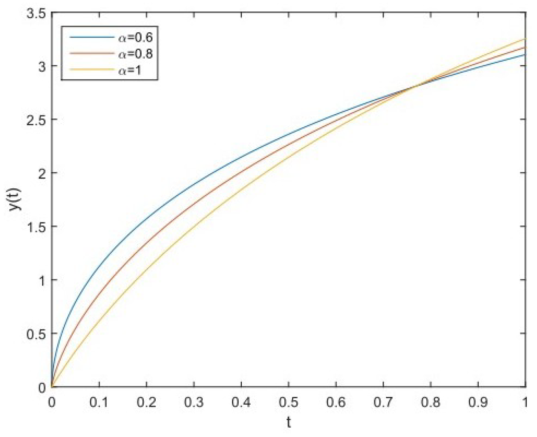
In Figure 1, we plot the solutions of Equation (20) for $\alpha =0.6,0.8,1.0$, that correspond to $\beta =0.5$, $\mu =\lambda =1$. The double sum was truncated with $n=50$ and $j=100$ using the time stepping condition of $h=e^{-3}$ in Matlab R2014b.

Figure 1 elicits the dynamics of a sphere immersed in an incompressible viscous fluid when $\beta$ is fixed and varying $\alpha .$ It is observed that the three models are increasing and coincide at two points $t=0$ and $t=0.8.$ For $0\le t\le 0.8$ the rate of increasing is inversely proportional to the magnitude of $\alpha$ but when $t>0.8$ this behaviour is reversed with $\alpha =1$ having the highest rate.

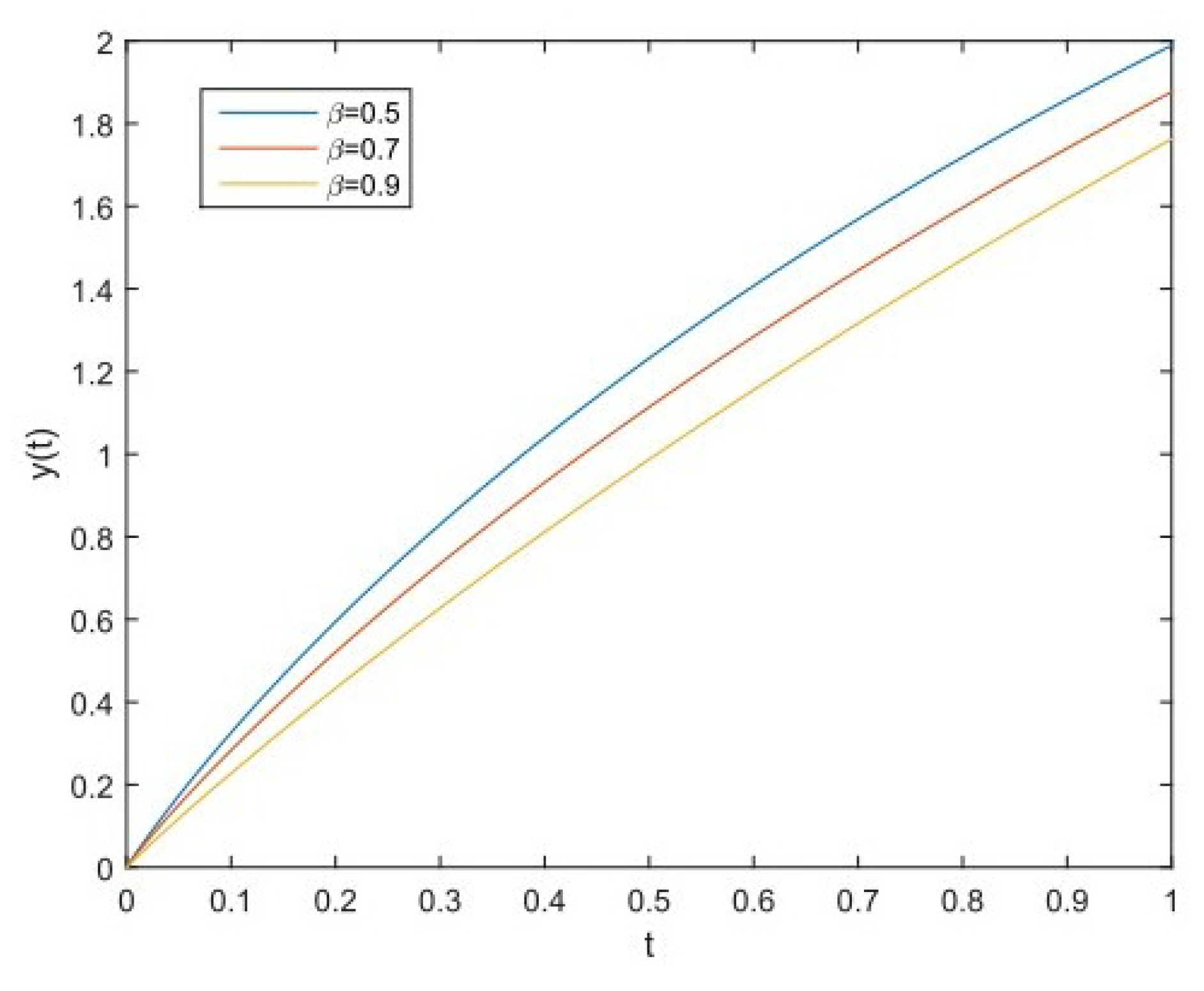
In Figure 2, we plot the solutions of Equation (20) for $\beta =0.5,0.7,0.9$, that correspond to $\alpha =1.0$, $\mu =\lambda =1$. The double sum was truncated with $n=50$ and $j=100$ using the time stepping condition of $h=e^{-3}$ in Matlab R2014b.

Figure 2 elicits the dynamics of a sphere immersed in an incompressible viscous fluid when $\alpha$ is fixed and varying $\beta .$ It is observed that the three models are increasing with the rate of increasing being inversely proportional to the magnitude of $\beta .$ In order words, as $\beta$ approaches 1 the solution becomes slower in the time frame $0\le t\le 1.$

Corollary 2.

If $y\left(0\right)=0$, $y^{\prime }\left(0\right)=0$ in Theorem 2 and

$$f\left(t\right)=\left\{\begin{array}{cc}2,\hfill & 0\le t\le 1,\hfill \\ 0,\hfill & t>1.\hfill \end{array}\right.$$

That is, the initial displacement and velocity was zero and an external force of 2 units was applied on the body for 1-time unit and then stopped. Then the solution reduces to

$$y\left(t\right)=\left\{\begin{array}{cc}2{\displaystyle \sum _{n=0}^{\infty }}{\displaystyle \sum _{j=0}^{\infty }}{(-\lambda )}^n{(-\mu )}^j\frac{\Gamma (n+j+1)}{\Gamma \left[\right(n+1)\alpha +(\alpha -\beta )j+1]n!j!}{t}^{(n+1)\alpha +(\alpha -\beta )j},\hfill & 0\le t\le 1,\hfill \\ 0,\hfill & t>1.\hfill \end{array}\right.$$

(21)

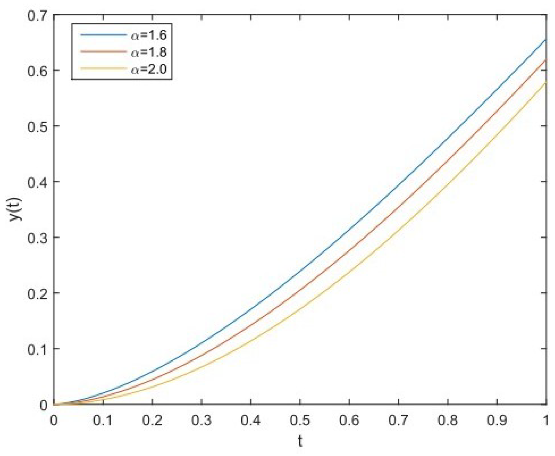
In Figure 3, we plot the solutions of Equation (21) for $\alpha =1.6,1.8,2.0$ that corresponds to $\beta =1.5$, $\mu =\lambda =0.5$. The double sum was truncated with $n=50$ and $j=100$ using the time stepping condition of $h=0.01$ in Matlab R2014b.

Figure 3 elicits the dynamics of an oscillatory pendulum process with fractional damping when $\beta$ is fixed and varying $\alpha .$ It is observed that the three models are increasing with the rate of increasing being inversely proportional to the magnitude of $\alpha .$ In order words, as $\alpha$ approaches 2 the solution becomes slower within the time frame $0\le t\le 1.$

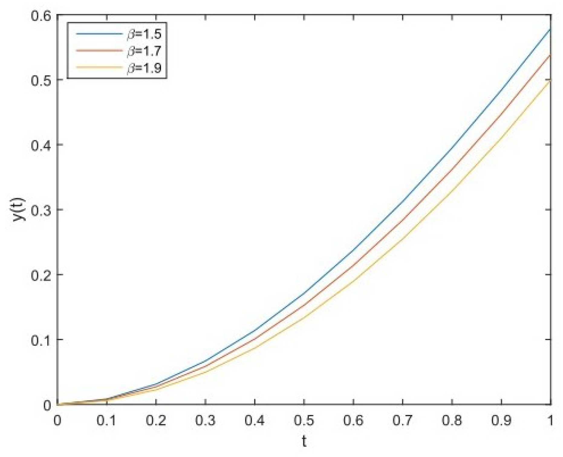
In Figure 4, we plot the solutions of Equation (21) for $\beta =1.5,1.7,1.9$, that correspond to $\alpha =2.0$, $\mu =\lambda =1$. Here again, the double sum was truncated with $n=50$ and $j=100$ using the time stepping condition of $h=0.01$ in Matlab R2014b.

Figure 4 elicits the dynamics of an oscillatory pendulum process with fractional damping when $\alpha$ is fixed and varying $\beta .$ It is observed that the three models are increasing with the rate of increasing being inversely proportional to the magnitude of $\alpha .$ In order words, as $\beta$ approaches 2 the solution becomes slower within the time frame $0\le t\le 1.$

5. Conclusions

In this article, we give analytic approach to solutions of the general fractional Caputo derivative differential equation models for the dynamics of a sphere immersed in an incompressible viscous fluid and oscillatory process with fractional damping using Laplace transform method. We studied the effects of fixing one of the fractional indices while varying the other as particular examples. It was observed that for $0\le t\le 0.8$ the rate of increasing of the solutions was inversely proportional to the magnitude of $\alpha$ but when $t>0.8$ this behaviour was reversed with $\alpha =1$ having the highest rate for a fixed $\beta$. Similar, behaviour was also observed for when $\alpha$ was fixed.

References

- Podlubny, I.; Magin, M.; Trymorush, I. Historical survey Niels Henrik Abel and the birth of fractional calculus. Fract. Calc. Appl. Anal. 2017, 20, 1068–1075. [Google Scholar] [CrossRef]
- Sergei, F.; Vladimir, C.; Toshiyuki, H. Application of Fractional Differential Equations for Modeling the Anomalous Diffusion of Contaminant from Fracture into Porous Rock Matrix with Bordering Alteration Zone. Transp. Porous Media 2010, 81, 187–205. [Google Scholar] [CrossRef]
- Hassan, F.; Zolotas, A. Impact of fractional order methods on optimized tilt control for rail vehicles. Fract. Calc. Appl. Anal. 2017, 20, 765–789. [Google Scholar] [CrossRef]
- Singh, J.; Kumar, D.; AlQurashi, M.; Baleanu, D. A Novel Numerical Approach for a Nonlinear Fractional Dynamical Model of Interpersonal and Romantic Relationships. Entropy 2017, 19, 375. [Google Scholar] [CrossRef]
- Fallahgoul, H.A.; Fabozzi, S.M.; Frank, F.J. Fractional partial differential equation and option pricing. In Fractional Calculus and Fractional Processes with Applications to Financial Economics; Fallahgoul, H.A., Focardi, S.M., Fabozzi, F.J., Eds.; Academic Press: Cambridge, MA, USA, 2017; pp. 59–80. [Google Scholar]
- Singh, J.; Kumar, D.; Hammouch, Z.; Atangana, A. A fractional epidemiological model for computer viruses pertaining to a new fractional derivative. Appl. Math. Comput. 2018, 316, 504–515. [Google Scholar] [CrossRef]
- Fouda, M.E.; Elwakil, A.S.; Radwan, A.G.; Maundy, B.J. Fractional-Order Two-Port Networks. Math. Probl. Eng. 2016, 2016. [Google Scholar] [CrossRef]
- Kilbas, A.A.; Srivastava, H.M.; Trujillo, J.J. Theory and Applications of Fractional Differential Equations; Elsevier: New York, NY, USA, 2006; Volume 204, pp. 1–523. [Google Scholar] [CrossRef]
- Kumar, D.; Singh, J.; Baleanu, D.; Sushila, J. Analysis of regularized long-wave equation associated with a new fractional operator with Mittag-Leffler type kernel. Phys. A Stat. Mech. Its Appl. 2018, 492, 155–167. [Google Scholar] [CrossRef]
- Li, Q.; Zhou, Y.; Zhao, X.; Ge, X. Dynamic Hedging Based on Fractional Order Stochastic Model with Memory Effect. Math. Probl. Eng. 2016, 2016. [Google Scholar] [CrossRef]
- Yanxin, W.; Li, Z. Solving nonlinear Volterra integro-differential equations of fractional order by using Euler wavelet method. Adv. Differ. Equ. 2017, 27. [Google Scholar] [CrossRef]
- Kilbas, A.; Trujillo, J. Differential equations of fractional order: Methods results and problem–I. Appl. Anal. 2001, 78, 153–192. [Google Scholar] [CrossRef]
- Mustapha, K.; Abdallah, B.; Furati, K.; Nour, M. A discontinuous Galerkin method for time fractional diffusion equations with variable coefficients. Numer. Algorithms 2016, 73, 517–534. [Google Scholar] [CrossRef]
- Li, Z.; Zhu, W. Fractional series expansion method for fractional differential equations. Int. J. Numer. Methods Heat Fluid Flow 2015, 25, 1525–1530. [Google Scholar] [CrossRef]
- Aghili, A.; Ansari, A. Solving partial fractional differential equations using the FA-transform. Arab J. Math. Sci. 2013, 19, 61–71. [Google Scholar] [CrossRef]
- Klimek, M.; Dziembowski, D. Mellin Transform for Fractional Differential Equations with Variable Potential. In Nonlinear Science and Complexity; Machado, J., Luo, A., Barbosa, R., Silva, M.S., Figueiredo, L., Eds.; Springer: Dordrecht, The Netherlands, 2011; pp. 281–292. [Google Scholar] [CrossRef]
- Li, K.; Peng, J. Laplace transform and fractional differential equations. Appl. Math. Lett. 2011, 24, 2019–2023. [Google Scholar] [CrossRef]
- Zainal, N.H.; Kilicman, A. Solving Fractional Partial Differential Equations with Corrected Fourier Series Method. Abstr. Appl. Anal. 2014. [Google Scholar] [CrossRef]
- Kumar, D.; Singh, J.; Baleanu, D. A new numerical algorithm for fractional Fitzhugh–Nagumo equation arising in transmission of nerve impulses. Nonlinear Dyn. 2018, 91, 307–317. [Google Scholar] [CrossRef]
- Singh, J.; Rashidi, M.; Sushila, J.; Kumar, D. A hybrid computational approach for Jeffery–Hamel flow in non-parallel walls. Neural Comput. Appl. 2017, 1–7. [Google Scholar] [CrossRef]
- Mainardi, F. Fractional relaxation-oscillation and fractional diffusion-wave phenomena. Chaos Solitons Fractals 1996, 7, 1461–1477. [Google Scholar] [CrossRef]
- Podlubny, I. Fractional Derivatives and Integrals. In Fractional Differential Equations: An Introduction to Fractional Derivatives, Fractional Differential Equations, to Methods of Their Solution and Some of Their Applications; Podlubny, I., Ed.; Elsevier: New York, NY, USA, 1999; Volume 198, pp. 41–119. [Google Scholar] [CrossRef]
- Gorenflo, R.; Kilbas, A.; Mainardi, F.; Rogosin, S. Mittag-Leffler Functions, Related Topics and Applications; Springer: Berlin/Heidelberg, Germany, 2014. [Google Scholar]
- Jumarie, G. Laplace’s transform of fractional order via the Mittag-Leffler function and modified Riemann-Liouville derivative. Appl. Math. Lett. 2009, 22, 1659–1664. [Google Scholar] [CrossRef]
- Teodoro, G.S.; de Oliveira, E.C. Laplace transform and the Mittag-Leffler function. Int. J. Math. Educ. Sci. Technol. 2014, 45, 595–604. [Google Scholar] [CrossRef]
- Wright, E. On the Coefficients of Power Series Having Exponential Singularities. J. Lond. Math. Soc. 1933, 8, 71–79. [Google Scholar] [CrossRef]
- Wright, E. The asymptotic expansion of the generalized Bessel function. Proc. Lond. Math. Soc. (Ser. II) 1935, 38, 257–270. [Google Scholar] [CrossRef]
- Wright, E. The generalized Bessel function of order greater than one. Q. J. Math. 1940, 11, 36–48. [Google Scholar] [CrossRef]
- Gorenflo, R.; Luchko, Y.; Mainardi, F. Analytic properties and applications of Wright functions. Fract. Calc. Appl. Anal. 1999, 2, 383–414. [Google Scholar]
- Prajapat, J. Certain geometric properties of the Wright function. Integral Transform. Spec. Funct. 2015, 26, 203–212. [Google Scholar] [CrossRef]
- Paneva-Konovska, J. From Bessel to Multi-Index Mittag-Leffler Functions: Enumerable Families, Series in Them and Convergence; World Scientific Publishing Europe: London, UK, 2016; pp. 1–228. [Google Scholar]
- Sandev, T.; Tomovski, Z.; Dubbeldam, J.L. Generalized Langevin equation with a three parameter Mittag-Leffler noise. Phys. A Stat. Mech. Its Appl. 2011, 390, 3627–3636. [Google Scholar] [CrossRef]
- Sandev, T. Generalized Langevin equation and the Prabhakar derivative. Mathematics 2017, 5, 66. [Google Scholar] [CrossRef]
- Sandev, T.; Metzler, R.; Tomovski, Z. Correlation functions for the fractional generalized Langevin equation in the presence of internal and external noise. J. Math. Phys. 2014, 55, 023301. [Google Scholar] [CrossRef]
- Saxena, R.; Mathai, A.; Haubold, H. Unified fractional kinetic equation and a fractional diffusion equation. J. Astrophys. Space Sci. 2004, 209, 299–310. [Google Scholar] [CrossRef]
Figure 1.
Dynamics of a sphere in an incompressible viscous fluid (Fixed .
Figure 2.
Figure 3.
Dynamics of an oscillatory pendulum with fractional damping (Fixed .
Figure 4.
© 2018 by the authors. Licensee MDPI, Basel, Switzerland. This article is an open access article distributed under the terms and conditions of the Creative Commons Attribution (CC BY) license (http://creativecommons.org/licenses/by/4.0/).
Share and Cite
MDPI and ACS Style
Zakariya, Y.F.; Afolabi, Y.O.; Nuruddeen, R.I.; Sarumi, I.O. Analytical Solutions to Fractional Fluid Flow and Oscillatory Process Models. Fractal Fract. 2018, 2, 18. https://doi.org/10.3390/fractalfract2020018
AMA Style
Zakariya YF, Afolabi YO, Nuruddeen RI, Sarumi IO. Analytical Solutions to Fractional Fluid Flow and Oscillatory Process Models. Fractal and Fractional. 2018; 2(2):18. https://doi.org/10.3390/fractalfract2020018
Chicago/Turabian StyleZakariya, Yusuf F., Yusuf O. Afolabi, Rahmatullah I. Nuruddeen, and Ibrahim O. Sarumi. 2018. "Analytical Solutions to Fractional Fluid Flow and Oscillatory Process Models" Fractal and Fractional 2, no. 2: 18. https://doi.org/10.3390/fractalfract2020018