Analytical Calculation of Falling Droplets from Cylindrical Capillaries ^†

Abstract

Existing investigations to estimate different properties of falling droplets are based on empirical data or complex mathematical approaches. This paper presents a new simple analytical approach to calculate selected properties of droplets, in particular the volume and frequency of falling droplets, out of a thin vertical cylindrical capillary. The fluid-reservoir is located above the capillary and provides a constant flow into the droplet. This leads to drop formation times less than one second. The results of the calculation are validated by numerical simulations and experiments.

1. Introduction

Tate, Rayleigh and Harkins & Brown (summarized in [1]) first investigated the mass of falling droplets in their experiments. Their aim was to predict the maximum droplet size under quasi-static conditions. Due to the observations of Neumann & Seeliger [2], who detected a change of the droplet volume with increasing flow rate in their experiments, these approaches are not applicable to the investigated droplet formation process with droplet formation times less than one second.

Other approaches are offered by Chesters [3], Eggers & Dupont [4] or Clanet & Lasheras [5]. They present much more extensive algorithms for the calculation of the shape of hanging and falling droplets using differential equations. These approaches are on the one hand much more accurate but on the other hand much more complicated than the approaches summarized in [1].

Comprehensively there is no approach with comparatively easy formulas to calculate the volume of falling droplets detaching from cylindrical capillaries. The aim of this paper is to present a simple analytical approach to close this gab and to verify this approach by experiments and numerical simulations.

2. Conservation of Momentum

To characterize the droplet formation process the momentum of the droplet has to be investigated. The momentum of the droplet only can change due to forces or other equivalent influences. The forces acting on the hanging droplet are the gravitational force

F_g = m·g

(1)

pulling the droplet downwards, on the one hand, and the surface force

F_sf,z = 2·π·R·σ·cos (α)

(2)

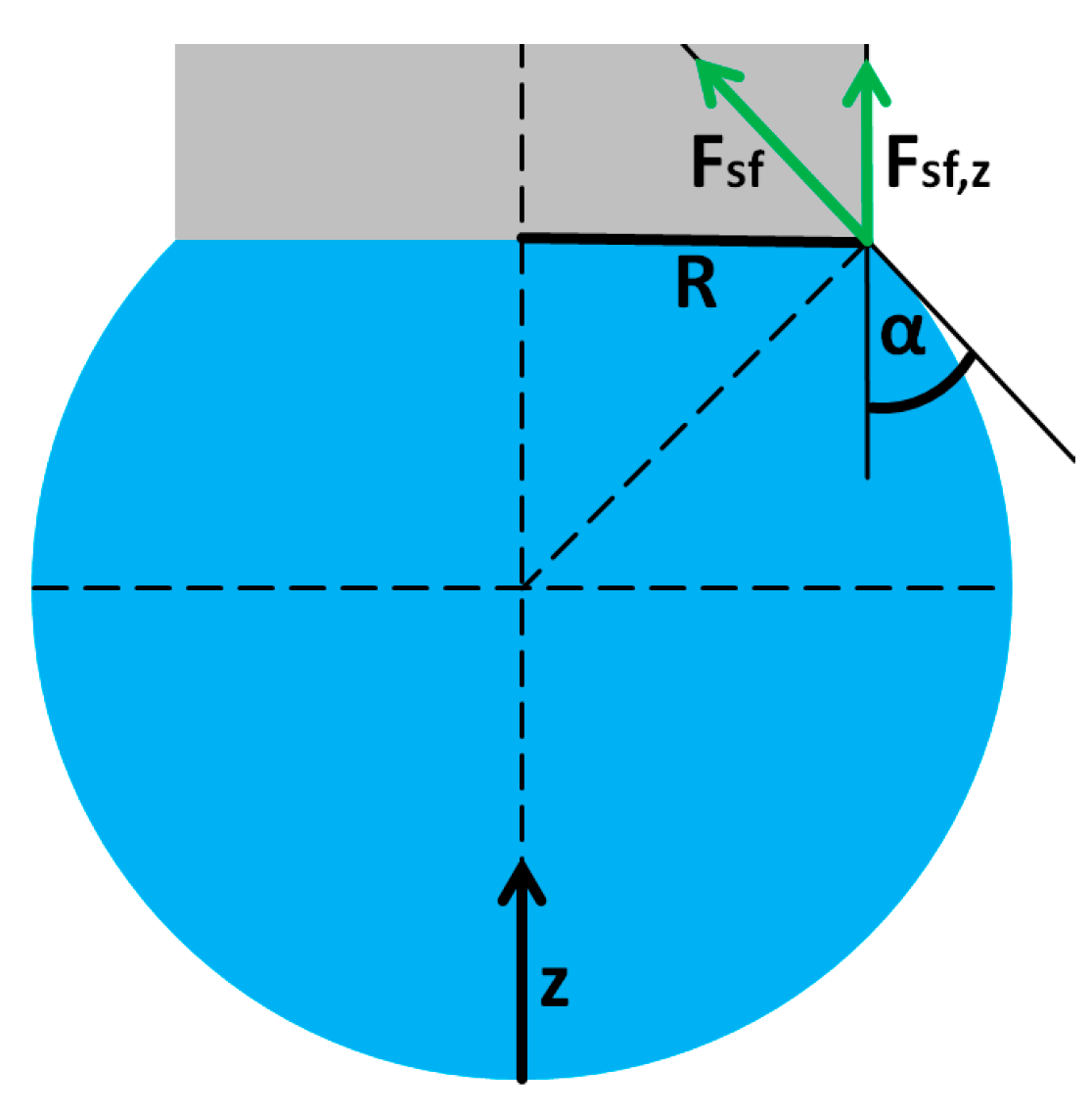
fixing the droplet to the capillary, on the other hand. In Equations (1) and (2) g is the gravitational constant, m the mass of the falling droplet, R the outer radius of the capillary, σ the surface tension and α the angle between the droplet and the outside of the capillary. The mentioned geometric characteristics are visualized in Figure 1.

The third influence on the change of the momentum, labeled with F_v, is based on the volumetric flow rate $\stackrel{.}{\mathrm{V}}$ streaming into the droplet with the velocity v, which is assumed to be constant:

$$\mathrm{Fv}=\mathsf{\rho }·\stackrel{.}{\mathrm{V}}·\mathrm{v}$$

(3)

This flow rate provides the fluid needed for the growth of the droplet. ρ is the density of the fluid.

Starting from the momentum I of the droplet being zero and assuming the droplet to remain unmoved (I = 0) the conservation of momentum follows out of the Equations (1)–(3):

dI/dt = F_sf,z − F_g − F_v = 0

(4)

Analyzing the droplet formation process leads to the insight that the droplet formation process can be divided up into three phases. In the first phase the surface force preponderates the downwards directed forces significantly and the shape of the droplet is nearly spherical. The angle α is increasing according to the increasing droplet volume and a critical value of α can be calculated for which F_sf,z and the sum of F_g and F_v are equal. In the second phase the angle α has to decrease with increasing droplet mass to ensure that the droplet stays fixed to the capillary. The second phase ends with the achievement of α = 0° due to the fact that no further increasing of the surface force F_sf,z is possible. In the described phases the momentum of the droplet due to its change of shape can be neglected which enables the calculation of both phases using the approach in Equation (4).

The third phase describes the necking of the droplet initialized by a minimal momentum of the droplet directly after the ending of the second phase. In this phase new effects according to the equations of Young-Laplace and Bernoulli are acting on the droplet. Eggers [6] presented an approach to estimate the necking time t which can be confirmed by the Buckingham π theorem. This approach will be used in this phase supplemented with an experimental correction factor k = 10:

t = k·R^3/2·ρ^1/2/σ^1/2,

(5)

with ρ being the density of the fluid and σ being the surface tension.

Using the presented approach allows the approximation of the droplet size and the time between two successive droplets using a simple analytical calculation. While dealing with Equation (4) the calculation of some parameters like the volumetric flow rate into the droplet is necessary. Therefore software like MatLab or SciLab is useful to reduce the calculation effort.

3. Numerical Simulations and Experimental Results

3.1. Numerical Simulations

To verify the presented approach the simulation software OpenFOAM for fluidic problems and the standard solver interFoam have been used to create two-dimensional cases. These cases differ from each other regarding the geometric conditions of the sample and the volumetric flow rate.

3.2. Experimental Setup

To generate experimental results a specific measurement setup was created using a RaspberryPi microcontroller and the according camera module. Using this setup it is possible to record the droplet formation process with 118 frames per second and a resolution of 640 × 480 pixels. The setup is illuminated by a LED with the power of 1 W. The capillary used in the experiments is of borosilicate glass and has an outer diameter of 0.88 mm, an inner diameter of 0.44 mm and a length of 20 mm. The fluid reservoir is located above the capillary and the fluid used in the experiments is deionized and degassed water. While recording the droplet formation process the temperature has to be monitored in order to correct the properties of the fluid used in the calculations.

3.3. Results

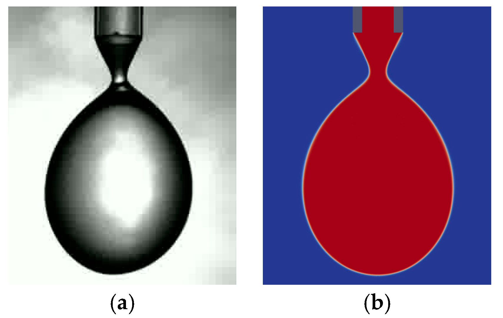
Figure 2 compares a droplet of water near its point of detachment from the capillary recorded with the experimental setup (a) and calculated numerically with OpenFOAM (b; red: water, blue: air). The figure illustrates the necking of the droplet in phase 3 of the previous described calculation approach and shows the accordance of experimental and simulation results in the droplet formation process.

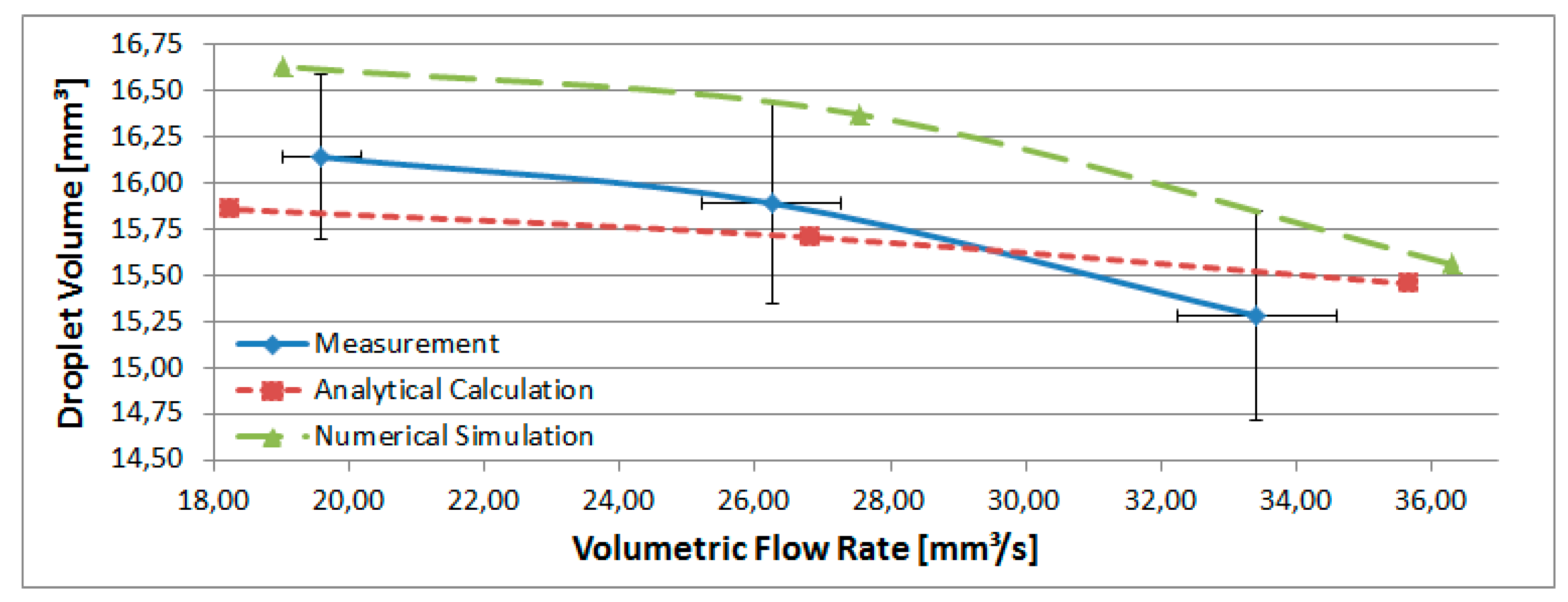
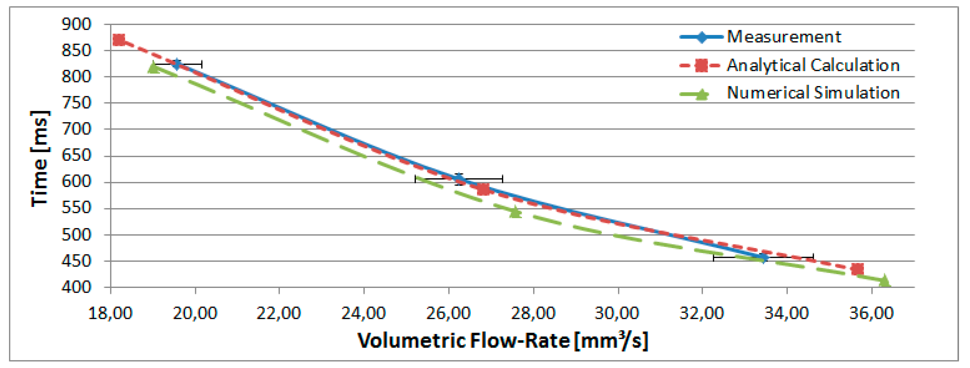
The Figure 3 and Figure 4 show the results of the calculation compared to the experimental and simulation results. The standard deviations of the volumetric flow rates are represented by horizontal error bars and the standard deviations of the measurement results, with a maximum value of ±4% of the average values which illustrates the accuracy of the experimental setup, are represented by vertical error bars. The measurement results fit to the analytical calculation within a deviation of ±2% for the droplet volume and a deviation of ±6% for the time between two successive droplets. Comparing the simulation results to the calculation leads to a deviation of ±5% for the droplet value and a deviation of ±7% for the time between two successive droplets.

4. Discussion and Conclusions

As presented in Section 3.3 the deviations between the measurement and the experimental results respectively between the measurement and the simulation results are less than ±7% within the investigated validity area of droplet formation times between 400 ms and 900 ms. This leads to the conclusion that it is possible to estimate the volume and time between two successive droplets with comparatively low effort. Using the presented approach for example in development processes for microfluidic dosing systems allows replacing complex simulations in order to reduce costs and time.

References

- Harkins, W.; Brown, F. The determination of surface tension (free surface energy), and the weight of falling drops: The surface tension of water and benzene by the capillary height method. J. Am. Chem. Soc. 1919, 41, 499–524. [Google Scholar] [CrossRef]
- Neumann, H.; Seeliger, R. Über die Abhängigkeit der Größe von Flüssigkeitstropfen von der Bildungsgeschwindigkeit. Z. Phys. 1939, 114, 571–578. [Google Scholar] [CrossRef]
- Chesters, A. An analytical solution for the profile and volume of a small drop or bubble symmetrical about a vertical axis. J. Fluid Mech. 1977, 81, 609–642. [Google Scholar] [CrossRef]
- Eggers, J.; Dupont, T. Drop formation in one-dimensional approximation of the navier-stokes equation. J. Fluid Mech. 1994, 262, 205–221. [Google Scholar] [CrossRef]
- Clanet, C.; Lasheras, J. Transition from dripping to jetting. J. Fluid Mech. 1999, 383, 307–326. [Google Scholar] [CrossRef]
- Eggers, J. Tropfenbildung. Phys. Bl. 1997, 53, 431–434. [Google Scholar] [CrossRef]
Figure 1.
Sketch to visualize the different geometric characteristics used in Equation (2). The vertical axis, labeled as z-axis, is set to be positive in the upwards direction.
Figure 2.
Hanging droplet near its point of detachment of the capillary: (a) Measurement; (b) Simulation.
Figure 3.
This figure shows the droplet volume depending on the volumetric flow rate into the droplet: The droplet volume increases with decreasing volumetric flow rate.
Figure 4.
This figure shows the time between two successive droplets depending on the volumetric flow rate into the droplet: The time increases with decreasing volumetric flow rate.
Publisher’s Note: MDPI stays neutral with regard to jurisdictional claims in published maps and institutional affiliations. |
© 2017 by the authors. Licensee MDPI, Basel, Switzerland. This article is an open access article distributed under the terms and conditions of the Creative Commons Attribution (CC BY) license (https://creativecommons.org/licenses/by/4.0/).
Share and Cite
MDPI and ACS Style
Hummel, S.; Bogner, M.; Haub, M.; Sägebarth, J.; Sandmaier, H. Analytical Calculation of Falling Droplets from Cylindrical Capillaries. Proceedings 2017, 1, 284. https://doi.org/10.3390/proceedings1040284
AMA Style
Hummel S, Bogner M, Haub M, Sägebarth J, Sandmaier H. Analytical Calculation of Falling Droplets from Cylindrical Capillaries. Proceedings. 2017; 1(4):284. https://doi.org/10.3390/proceedings1040284
Chicago/Turabian StyleHummel, Sebastian, Martin Bogner, Michael Haub, Joachim Sägebarth, and Hermann Sandmaier. 2017. "Analytical Calculation of Falling Droplets from Cylindrical Capillaries" Proceedings 1, no. 4: 284. https://doi.org/10.3390/proceedings1040284