Groundwater Modeling with Machine Learning Techniques: Ljubljana polje Aquifer ^†

Abstract

In this study a thorough analysis is conducted concerning the prediction of groundwater levels of Ljubljana polje aquifer. Machine learning methodologies are implemented using strongly correlated physical parameters as input variables. The results show that data-driven modelling approaches can perform sufficiently well in predicting groundwater level changes. Different evaluation metrics confirm and highlight the capability of these models to catch the trend of groundwater level fluctuations. Despite the overall adequate performance, further investigation is needed towards improving their accuracy in order to be comprised in decision making processes.

1. Introduction

To address challenges associated with climate resilience and sustainability principles, the importance of urban groundwater must be integrated into urban planning and design. Groundwater systems are dynamic and adjust continually to short-term and long-term changes in climate, groundwater withdrawal, and land use. Water level measurements from observation wells are the principal source of information about the hydrologic stresses acting on aquifers and how these stresses affect ground-water recharge, storage, and discharge. In this research we focus on Ljubljana polje aquifer.

Traditionally groundwater levels are modeled with process-based models, which rely on the profound knowledge of the observed system dynamics. They require many additional spatial data on geological and hydrological properties of the aquifer. On the other hand, in data-driven modeling with machine-learning techniques our model is based solely on the data and some domain-specific knowledge is incorporated in to the system via appropriate data transformation (within engineering of new attributes). The goal in such a scenario would be to predict groundwater levels based on temporal data inputs (historic groundwater and surface water level data, weather data and forecasts, land-use, groundwater withdrawal and other anthropogenic data) and outputs (groundwater level). The model captures underlying processes based on the data without additional expert user input. In our work we present the whole data-mining pipeline, including exploratory data analysis, data pre-processing and modeling, where we explore accuracy and other benefits of a variety of modeling techniques on the same dataset (from interpretable modeling techniques such as multivariate linear regression, linear SVM and decision trees to black-box models such as gradient boosted trees, random forests and artificial neural networks), which has rarely been reported in scientific literature for water-related scenarios.

Authors of [1] claimed already a decade ago that data-driven modeling has overcome the initial stage and the main objectives shifted from method development and testing to the construction of useful architectures and applications of data-driven modeling for decision makers, according to the availability of the data. In reality, however, machine learning is still seeking its way into the practice and many studies have been published recently, which are researching the usability of different machine learning algorithms. Time-series techniques (ARX, ARMAX, ARMA, ARIMA) and artificial neural network models have been tested in [2]. Random forests and maximum entropy have been tested in [3]. Sahoo et al. [4] focused on multilayer perceptron networks. With R² scores higher than 0.8 they claim that data-driven approach can be used as an alternative to process modeling techniques.

The Ljubljana polje aquifer has been studied extensively, mainly with process models [4,5,6,7]. The aquifer recharges mainly through infiltration of river water, infiltration of precipitation and in smaller fraction through lateral underground flow [8]. The latter is still not studied and understood well [9]. Therefore we can expect that appropriate data to model groundwater will be originating geographically within the aquifer (surface water levels, precipitation, etc.).

Machine learning models have not been studied in the Ljubljana polje aquifer, however some preliminary work has been reported on automatic data acquisition [10]. Markov chains have been used to model heterogeneity of the aquifer [11]. Machine learning models have been used to study geological-geomechanical properties of Ljubljana area [12].

2. Materials and Methods

2.1. Data and Data Acquisition

For data acquisition, we used Internet of Things (IoT) middleware which consists of four main components, named Retrievers, Collector, API Management and Watchdog. The infrastructure is able to retrieve data from the heterogeneous sources, transform it into a unified format, store it and finally expose it via standardized web services, so it is available to users for further processing. The service is further described in [13].

In the Water4Cities project we collect three different data sets from Ljubljana (Slovenia) and Skiathos (Greece): groundwater information, pump sensor data from Skiathos and weather data. Groundwater dataset contains data from 518 stations comprising 28 regions which measure groundwater levels. Data are collected since 1960 (with median frequency of one day); however, there are some stations that started operating later, or operated intermittently, which means some data are not available.

Weather data are refreshed once per day and contain temperatures (daily average, minima and maxima), location data, precipitation, snow blanket, new snow blanket, cloud cover and sun duration. Data from Ljubljana are available from 2010.

2.2. Modeling Approach

We are training a model that will be able to predict continuous groundwater level values based on a set of related attributes (weather data, available historic values of groundwater levels, etc.). We have collected data that combine all the related attributes and target value (groundwater level). Such a problem belongs to the field of supervised learning, more specifically—it is a regression problem.

There is a plethora of algorithms, capable of such a task; however, it is important that our experiments are designed in a way that will give useful and accurate results. Our initial experiments aimed at predicting absolute value of groundwater levels. This proved to be an inefficiently defined problem, since absolute water level depends strongly on long-term historic processes, which we cannot easily grasp with limited attribute vectors. We have, therefore, set our target value not to absolute groundwater level, but rather to the changes in groundwater levels. For each day we are trying to predict whether and how much the groundwater levels will rise or drop.

2.3. Data-Driven Modelling Algorithms

Groundwater level prediction is a regression problem. Based on available data (i.e., weather data, weather predictions, people-behavior model prediction, etc.) we are trying to generate the best possible continuous predictions for groundwater level change on a particular day. Data-driven algorithms use past data to learn the best approximation of an underlying process behind a particular phenomenon.

2.3.1. Linear Regression

One of the oldest and widely used methods is linear regression [14]. We are solving the following equation:

$$y=X\beta +ϵ,$$

(1)

where y is a vector of observed target values (in our case groundwater level or groundwater level change), X is a matrix that contains rows of independent variables—attributes (in our case weather, historic or other data), β is a parameter vector we are trying to learn and ε is a vector of errors. The goal is to learn parameter vector β in order to minimize errors on the validation set. There are many techniques for parameter estimation, the most well-known are based on least squares estimation.

2.3.2. Regression Trees, Random Forests and Gradient Boosting

Regression trees are an algorithm based on decision trees. When learning, we segment the attribute space into many different subspaces, where each particular subspace represented by a tree leaf has a value, which might be obtained simply by averaging all the samples from training set that belong to that leaf or by introducing another model (often linear regression) at each final node.

Regression trees work well in ensembles. Breiman [15] suggested to use ensembles of regression trees to improve prediction accuracy. Each regression tree is trained with a particular sub-sample of a data set (different attributes and different samples from original dataset are used). Final value is given by an average over the whole ensemble. The algorithm is popular as it is fast and easy to parallelize and has proven very successful in numerous applications in environmental data-driven modeling (and elsewhere).

Gradient boosting [16] also utilizes an ensemble of weak learners (usually trees) to provide final prediction, but it stacks them additively. In the first stage the algorithm approximates target values. In each subsequent stage the algorithm approximates pseudo-residuals (loss function differentials) from previous stage. An example of a simple loss function would be

$$L\left(y, F_m\left(x\right)\right)=\frac{1}{2}{\left(y-F_m\left(x\right)\right)}^2,$$

(2)

where y is true value and F_m(x) is the model prediction after m-th stage. Model prediction F_m(x) combines all the weak learners’ results. Gradient boosting is the state of the art method in various fields (i.e., in particle physics).

2.4. Evaluation Methods

We evaluate goodness of fit with root mean squared error (RMSE) and coefficient of determination (R²) metrics. We define them as follows:

$${\mathrm{R}}^2=1-\frac{{{\displaystyle \sum }}_{t=1}^n{\left(f_t-\overline{y}\right)}^2}{{{\displaystyle \sum }}_{t=1}^n{\left(y_t-\overline{y}\right)}^2}$$

(3)

$$\mathrm{RMSE}=\frac{1}{n}{{\displaystyle \sum }}_{t=1}^n(y_t-f_t)$$

(4)

$f_t$ represents prediction and $y_t$ true value at time t, $\overline{y}$ is average true value on the dataset, n is the number of data samples.

RMSE is a metric that can be easily interpreted in the scope of the use case as it is in the units of the target value. Its main disadvantage is that it cannot be compared across datasets. R² is invariant to the amplitude of the target value and can be compared in different scenarios.

We report performance of our algorithms by using 3-fold cross validation.

3. Results

3.1. Exploratory Data Analysis

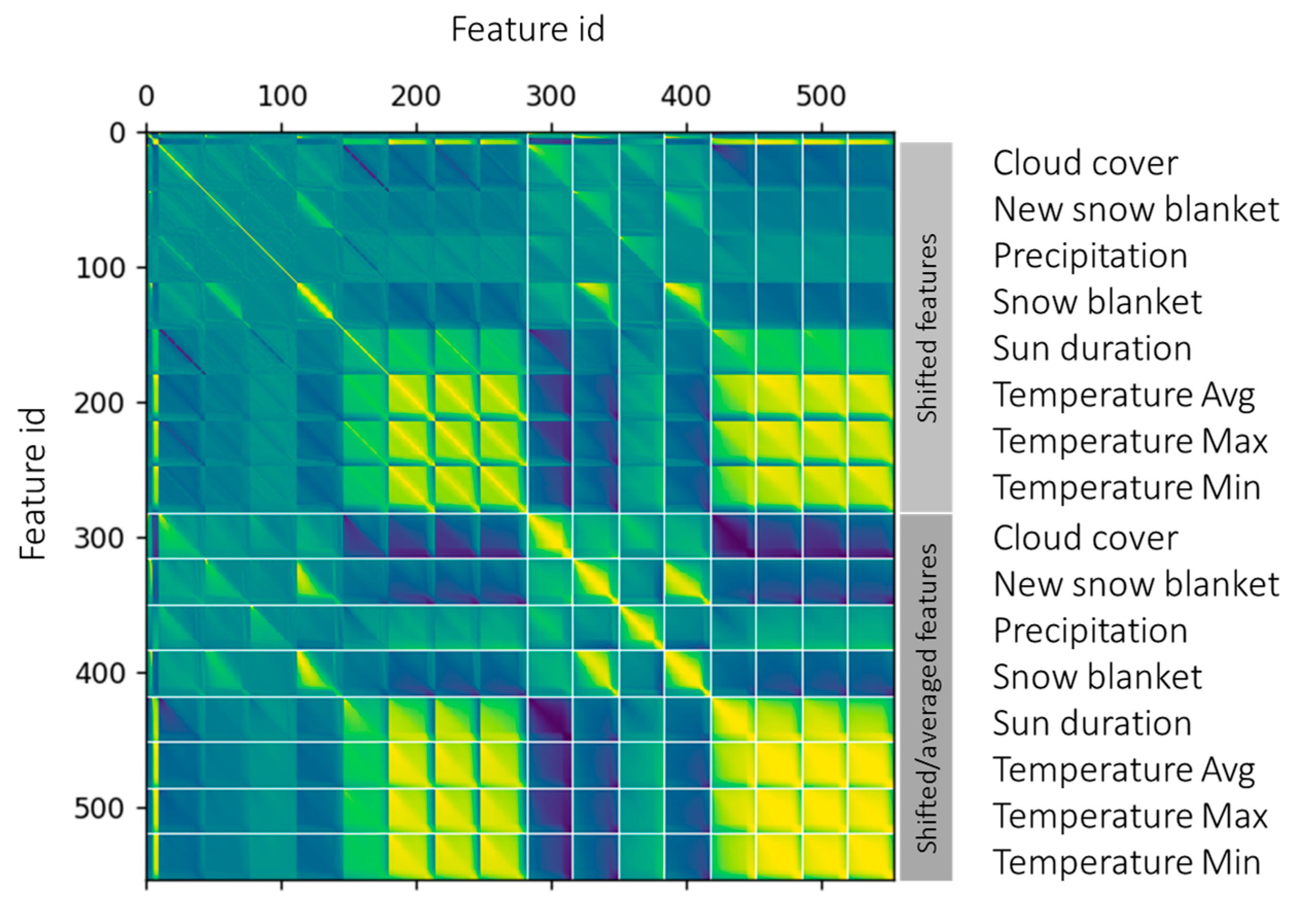
Initial part of the data mining process has been dedicated to feature engineering (engineering of new attributes). We have speculated that different weather phenomena are responsible for groundwater level dynamics: mainly precipitation, snow melting and weather in the whole study area. We have used raw values of all weather attributes (see Figure 1) and different derivatives. Firstly, we introduced time delay in the attribute as we speculated, that it takes time before surface water recharges the aquifer and secondly, we speculated that sums (or averages in the context of data-mining attributes) over multiple past days might play a significant role. Figure 1 depicts the correlation matrix of all 544 generated attributes.

Correlation matrix can be used in two ways. Firstly, we can read the correlations of particular attributes with our target variable (groundwater level daily change) and select the most correlated attributes to use in our models. Secondly, we can use it for filtering of highly correlated attributes. Highly correlated attributes will not bring additional knowledge to the model and might worsen model accuracy. Additionally, number of generated attributes is of the same magnitude as number of samples in our datasets, which might lead to overfitting of the models.

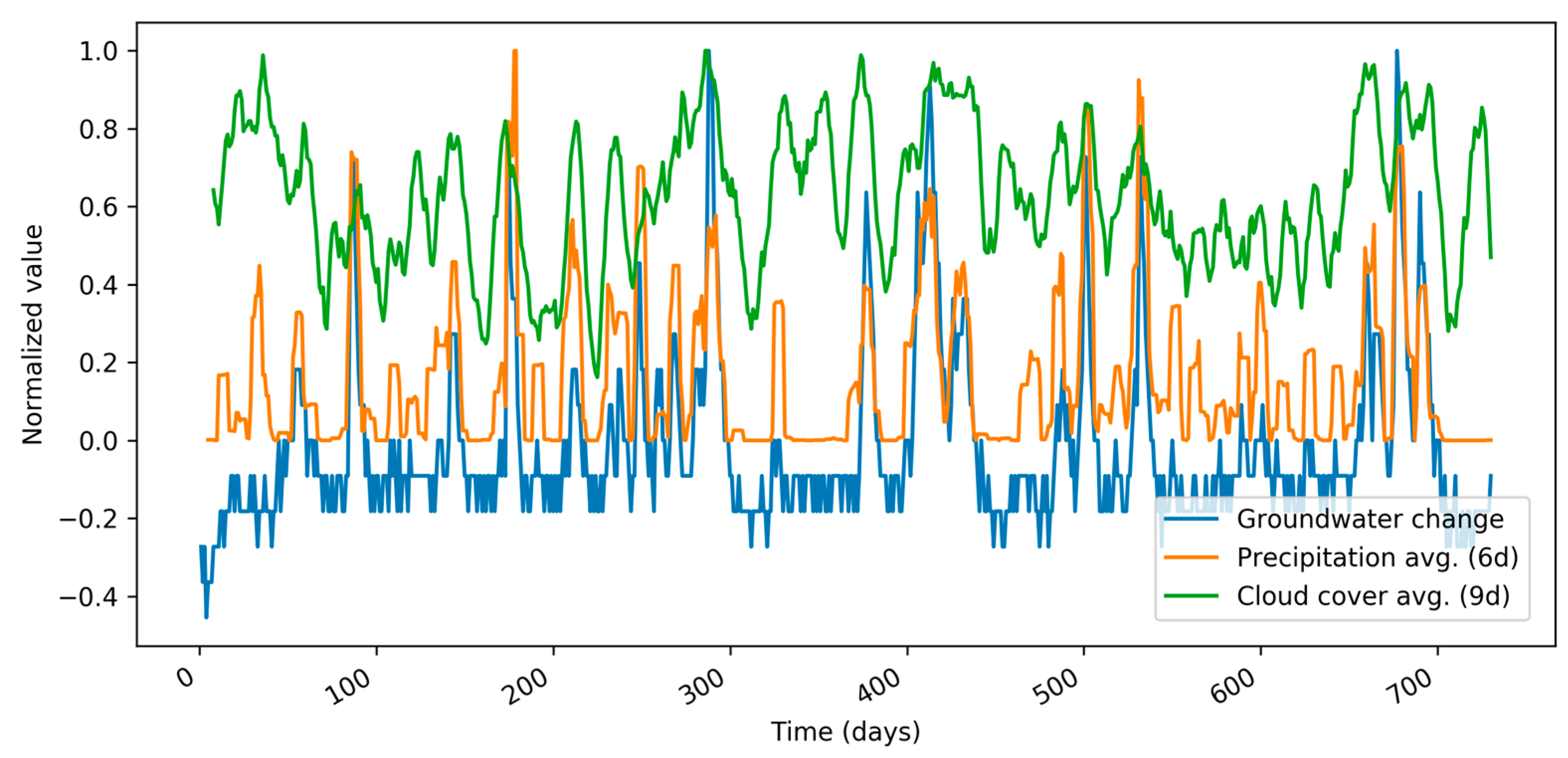
A pair of heterogeneous attributes that are strongly correlated to the target value (groundwater change) are depicted in Figure 2. The attributes are 6-day precipitation average and 9-day cloud cover average.

3.2. Modeling Results

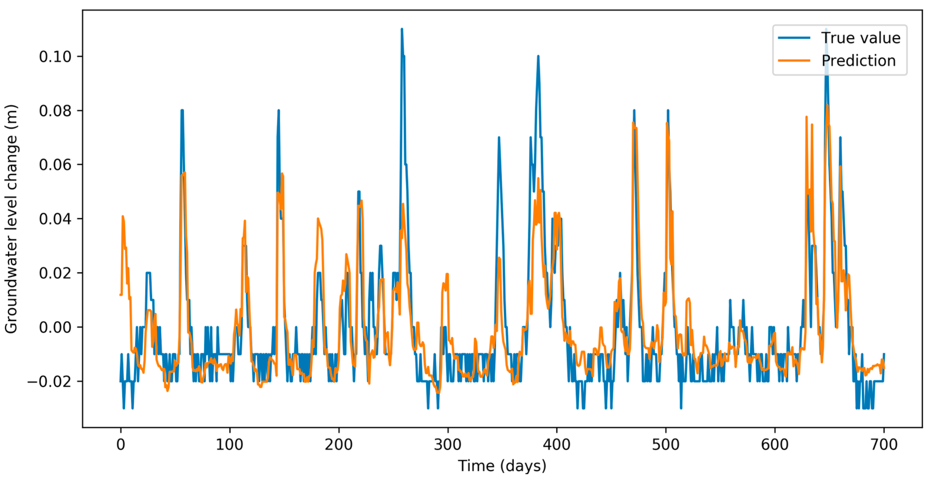
Final feature vectors have been composed of candidates from top-30 correlated attributes. 13 best and mutually least correlated features (according to Figure 1) have been selected. Modeling results are depicted in Figure 3 and Figure 4. Figure 3 depicts comparison between groundwater level change (blue) and its prediction (orange). Visually, we can identify very good fit between the two, which shows that the model explains most of the fluctuations. We can observe that some extreme peaks in groundwater changes are not explained by our features. Further work is needed to identify those.

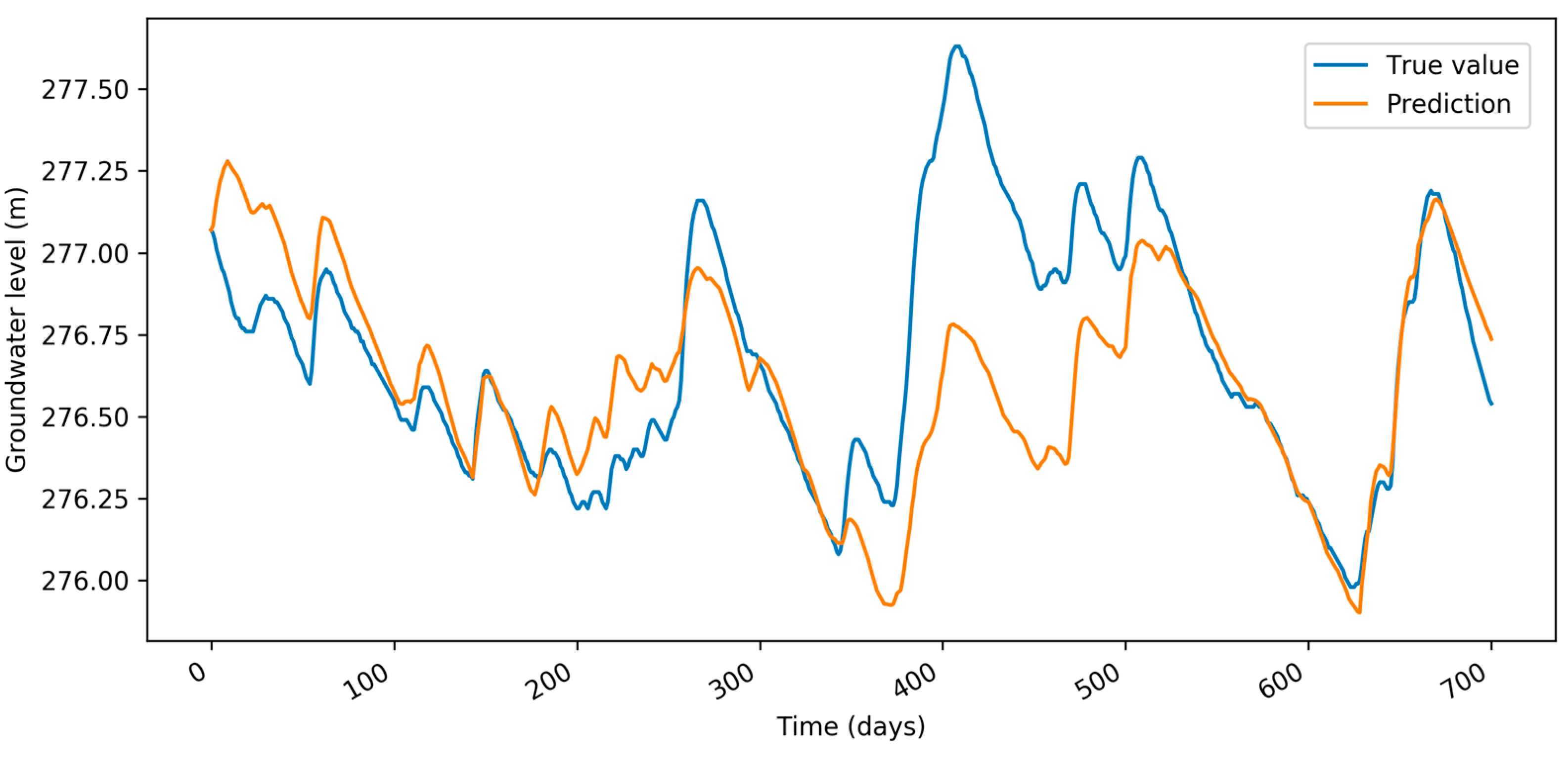
Figure 4 depicts comparison between absolute groundwater level based on our model (orange) and true values (blue). Absolute values are calculated based on summing up groundwater level change predictions over time. We can see that the shape of the orange line reflects dynamics in the blue line, but absolute values might include big differences.

Table 1. Modeling results of groundwater level change prediction, based on weather data. 4 different algorithms were used. Each method has been run on a dataset of 5 different nodes from Ljubljana polje aquifer.

Algorithm	R2	RMSE
Linear regression	0.624	$2.23\times$10−4
Decision trees	0.415	$3.46\times$10−4
Random forest	0.609	$2.31\times$10−4
Gradient boosting	0.644	$2.11\times$10−4

presents evaluation metrics on the same data-set using 4 different modeling algorithms: linear regression, regression trees, random forests and gradient boosting. Gradient boosting is the superior method.

4. Discussion

In this work, we have demonstrated that data-driven modeling techniques within water-management domain can yield useful results with models that are computationally and implementation-wise much less complicated than the current state-of-the-art process-driven models. We have conducted experiments on Ljubljana polje aquifer groundwater data.

Based on location of the groundwater level sensors we have achieved satisfactory results, however—we have encountered some anomalies, where our models were unable to model the underlying dynamics of the aquifer. Most of the anomalies are the drought between 2011 and 2012, when groundwater level dropped close to an apparent minimal level. As the models have no information about current groundwater level, they were unable to catch this dynamics. Additionally, some sensors placed near the surface water sources seem to fluctuate close to some predetermined level and are not so much dependent on weather itself. All these anomalies could be handled with additional features, better understanding of the aquifer dynamics and more precisely defined use-case scenarios.

Future work includes many interesting research directions. Firstly, a systematic study on a wide variety of water-management use cases should be performed. Different data-driven approaches should be tested with a wide variety of algorithms (SVM regression, kNN, multi-layer perception …). So far, researchers have used arbitrary machine learning methods (often they have not even compared them to other available methods). The aim of the study would be to identify the best methods within the domain.

As deep learning is becoming more popular in multiple fields, the methods reported in recent water-management literature, should be further investigated and improved. Different neural network architectures should be tested. Experience from other fields (i.e., particle physics), which deal with similar streams, show that we can often improve state-of-the-art results with deep learning; however, improvement might not be significant and computationally cheaper methods (like random forests or gradient boosting) can achieve competitive results.

Another approach towards computationally less demanding (and thus so called green) methods would be the implementation of stream learning techniques. IoT paradigm is expected to flourish within the water-management practice in the years to follow. Such approaches, which would involve a wide range of prediction models, can be beneficial.

In many domains, such as energy management, data-driven approaches have been pushed aside due to different privacy-related issues. Similar tendency is noticed in water management field. Therefore, it is crucial to stimulate relevant stake-holders to use the methodologies in order to improve decision making processes within their respective organizations. Implementation of such methodologies is an important step towards integration of intelligent decision support systems.

Additionally, a thorough evaluation and comparison of process and data-driven models should be conducted, in order to register limitations, advantages and usability of the latter in real-life scenarios.

5. Conclusions

In this study we conduct an analysis for forecasting groundwater levels. Four data-driven methodologies are tested; namely, linear regression, decision trees, random forests, and gradient boosting. Prediction of groundwater level change proved to be a better approach in comparison to the prediction of absolute groundwater levels. All models tested are multivariate and the predictors inserted are: cloud cover, snow blanket, new snow blanket, precipitation, sunlight duration, and average, maximum and minimum temperatures. A variable delay between groundwater change and the predictors was introduced to simulate the actual dynamics of aquifer recharge. Cloud cover and precipitation were chosen to better predict the target attribute. Gradient boosting resulted as the best fitting method with R² = 0.644 and RMSE = 2.11$\times$10⁻⁴. According to the results, the method catches adequately the trend but is not catching some groundwater level high peaks.