Inverse Analysis for Estimating Temperature and Residual Stress Distributions in a Pipe from Outer Surface Temperature Measurement and Its Regularization †

Department of Mechanical Engineering, Faculty of Science and Engineering, Setsunan University, 17-8, Ikedanakamachi, Neyagawa, Osaka 572-8508, Japan
*
Author to whom correspondence should be addressed.
†
Presented at the 18th International Conference of Experimental Mechanics, Brussels, Belgium, 1–5 July 2018.
Proceedings 2018, 2(8), 407; https://doi.org/10.3390/ICEM18-05284
Published: 30 May 2018
(This article belongs to the Proceedings of The 18th International Conference on Experimental Mechanics)
Abstract
:This paper presents an inverse analysis method for estimating the temperature and thermal residual stress distributions in the pipe from the temperature history measured on the outer surface. A regularization method was introduced. It is found from numerical simulations that the proposed inverse analysis method with regularization is useful for obtaining a reasonable estimate of the inner surface temperature and thermal stress.
1. Introduction
It was revealed that fluctuation of fluid temperature in a pipe may induce high cycle thermal fatigue in the pipe, which sometimes results in fracture of the pipe [1,2,3,4]. The information about the temperature and thermal residual stress distributions is important to prevent the high cycle thermal fatigue. It is, however, difficult to measure the temperature in the pipe directly. The monitoring of the temperature on accessible outer surface is promising to solve the problem. This paper presents an inverse analysis method for estimating the temperature and thermal stress distributions in the pipe from the temperature history measured on the outer surface. A regularization method is proposed for obtaining a reasonable solution.
2. Mathematical Structure of Temperature Distribution in a Thin Pipe
Consider a pipe subjected to thermal fluctuation on its inner surface. As an extreme the thickness of the pipe h is assumed to be small compared with the radius of the pipe. The governing equation of temperature distribution is expressed by the following equation of thermal conduction.
Here x is the distance from the inner surface of the pipe, t is time and the k is the thermal diffusivity. Suppose that the inner surface temperature is given by a sinusoidal function of angular velocity as:
Taking account of the fact that the temperature is supposed to decay with x, we are interested in the following solution of Equation (1):
Then the temperature on the outer surface of the pipe is given as,
From Equations (2) and (4) it is seen that the amplitude of the outer surface temperature compared with that of the inner surface temperature is reduced by ratio R, and that the phase of the outer surface temperature is delayed by Δp compared to the inner surface temperature, and R and Δp are given as [5,6]:
3. Inverse Method for Estimating Temperature and Thermal Stress Distributions
When the temperature on the outer surface is expressed by periodical function of time t with cycle time T, is expressed by the Fourier expansion as:
Based on the mathematical relationship between the temperature on the outer surface and that on the inner surface discussed in the foregoing section, the inner surface temperature history is estimated by amplifying by a ratio 1/R and also by advancing the phase by Δp:
Here the reduction ratio Rm and the phase lag Δpm for the m-th term in the series are expressed as,
4. Regularization Method
The reduction factor Rm given by Equation (9) is very small for very high frequency component, or large value of m. Then high frequency fluctuation measured on the outer surface is exaggerated in the estimation of the inner surface temperature history. In the presence of measurement noise, incorrect high frequency components deteriorate the estimation. We introduce a regularization method to exclude the incorrect components. This limit is determined by considering the effect of noise to the coefficient of the Fourier coefficients. When the error in outer surface temperature measurement is of the order of δ, the expected amplitude of the Fourier coefficient is in the order of . Then regularization was conducted by ignoring the Fourier coefficient of the outer surface temperature, whose absolute value is smaller than this value.
5. Estimation of Thermal Stress Distribution
The total strain is composed of thermal strain and mechanical strain :
Here E is Young’s modulus and denotes thermal stress. The total strain is independent of x due to uniform deformation of the long pipe. Then the equilibrium of thermal stress gives rise to the following expression of the thermal stress.
6. Numerical Simulations
Numerical simulations were made to examine the applicability of the proposed method. A pipe made of type 316 stainless steel is considered. The thermal diffusivity is m2/s. Young’s modulus is 193 GPa. The thickness of the pipe h is 0.015 m, the cycle time T is 100 s. It is assumed that the inner surface temperature is given by superposing three waves, whose amplitude and cycle period are given in Table 1. As the error in the outer surface temperature measurement, 2 °C, 5 °C and 8 °C were employed. Artificial error was introduced using uniform random number.
Figure 1a–c show the inner surface temperature history by applying the estimation method without regularization for the measurement error of 2 °C, 5 °C and 8 °C, respectively. It is seen that the estimated inner surface temperature (blue line) is fluctuated around the real one (red line). As the noise level is increased high frequency components give rise to big fluctuation in the estimated inner surface temperature history. The fluctuation is pronounced for large measurement error.
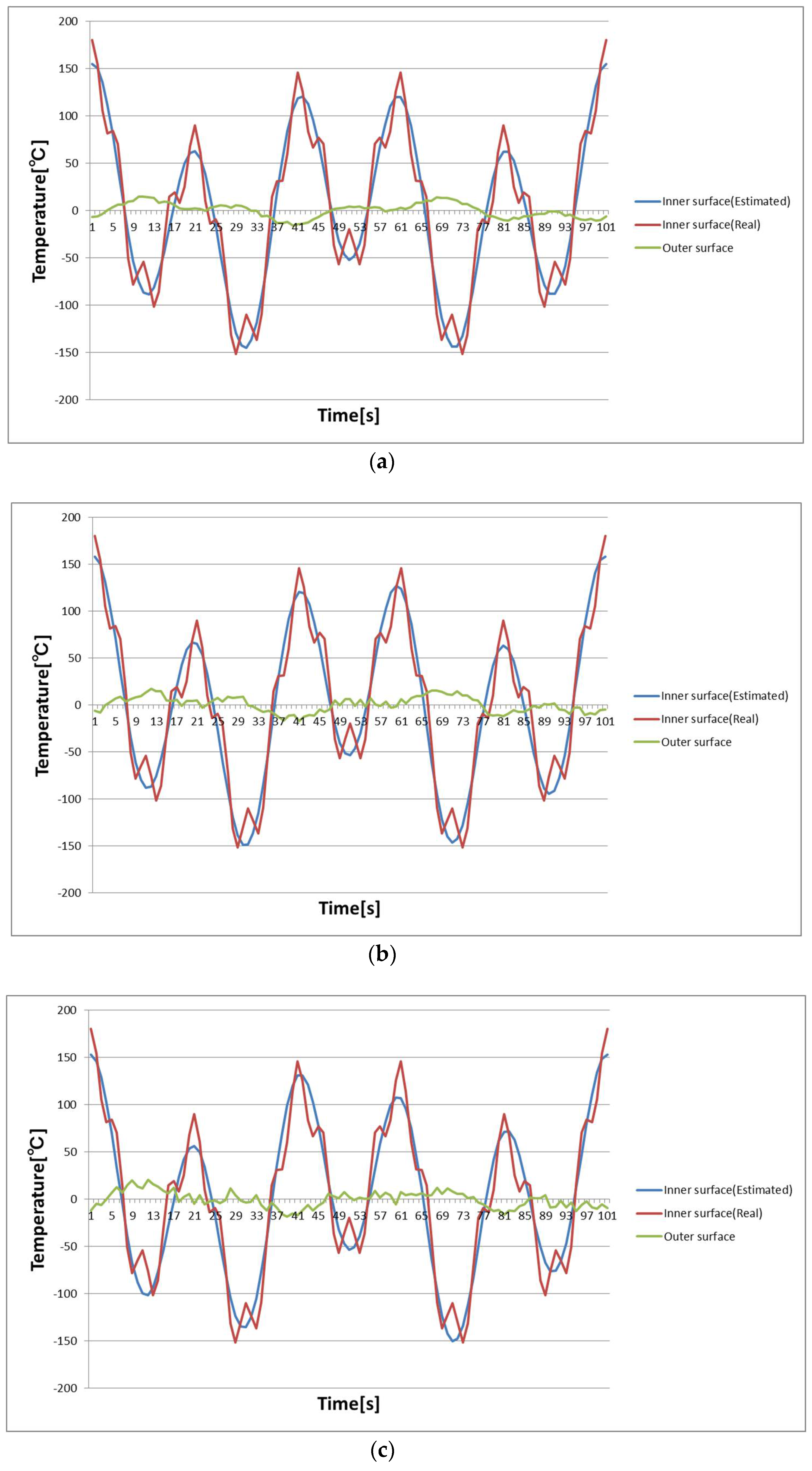
Figure 2a–c show the inner surface temperature history by applying the estimation method with regularization for the measurement error of 2 °C, 5 °C and 8 °C, respectively. It is found that a reasonable estimation is made by applying the regularization method even in the existence of considerable observation error, although the information about the very high frequency component is lost.
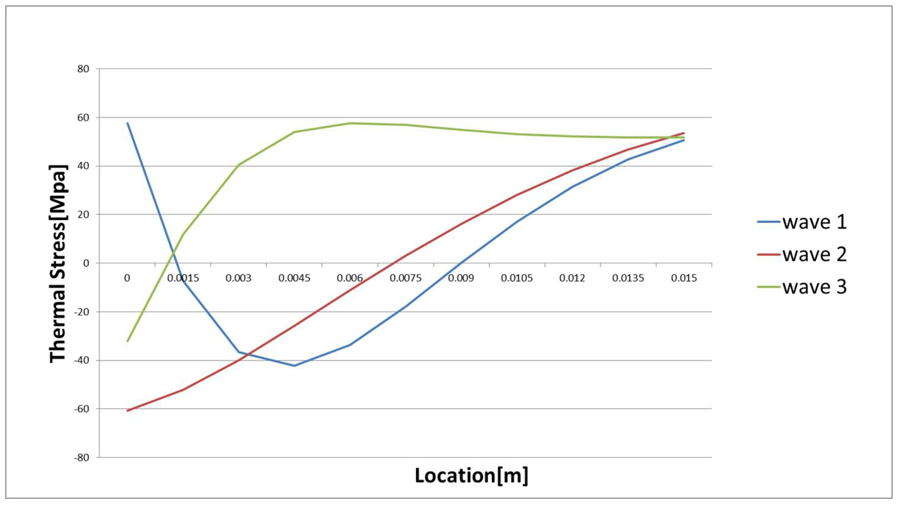
Using the temperature history the estimation of the thermal stress in the pipe was made. As an example the thermal stress at t = 5 s for the three waves examined in the foregoing are shown in Figure 3. Thermal fatigue life can be evaluated using the estimated thermal stress and counting the number of cycles.
7. Conclusions
An inverse analysis method was presented for estimating the temperature and thermal stress distributions in the pipe from the temperature history measured on the outer surface. Regularization method was introduced. It was found that the proposed inverse analysis method with regularization was useful for obtaining a reasonable estimate of the inner surface temperature and thermal stress.
References
- Meeker, J.; Segall, A.E.; Gondar, E. An Inverse Method for the Determination of Thermal Stress-Intensity Factors under Arbitrary Thermal-Shocks. J. Press. Vessel Technol. Trans. ASME 2018, 130, 041206. [Google Scholar] [CrossRef]
- Segall, A.E.; Engels, D.; Hirsh, A. Transient Surface Strains and the Deconvolution of Thermoelastic States and Boundary Conditions. J. Press. Vessel Technol. Trans. ASME 2019, 131, 011201. [Google Scholar] [CrossRef]
- Kasahara, N.; Takasho, H.; Yacumpai, A. Structural Response Function Approach for Evaluation of Thermal Striping Phenomena. Nucl. Eng. Des. 2002, 212, 281–292. [Google Scholar] [CrossRef]
- Kamide, H.; Igarashi, M.; Kawashima, S.; Kimura, N.; Hayashi, K. Study on Mixing Behavior in a Tee Piping and Numerical Analysis for Evaluation of Thermal Striping. Nucl. Eng. Des. 2009, 239, 58–67. [Google Scholar] [CrossRef]
- Ioka, S.; Kubo, S.; Ochi, M.; Hojo, K. Development of Inverse Analysis Method of Heat Conduction and Thermal Stress for Elbow (Part I). J. Press. Vessel Technol. Trans. ASME 2016, 138, 051202. [Google Scholar] [CrossRef]
- Hojo, K.; Ochi, M.; Ioka, S.; Kubo, S. Development of Inverse Analysis Method of Heat Conduction and Thermal Stress for Elbow—Part II. J. Press. Vessel Technol. Trans. ASME 2016, 138, 051207. [Google Scholar] [CrossRef]
Figure 1.
Estimated temperature variation on inner surface without regulation. (a) Observation noise of 2 °C; (b) Observation noise of 5 °C; (c) Observation noise of 8 °C.
Figure 1.
Estimated temperature variation on inner surface without regulation. (a) Observation noise of 2 °C; (b) Observation noise of 5 °C; (c) Observation noise of 8 °C.
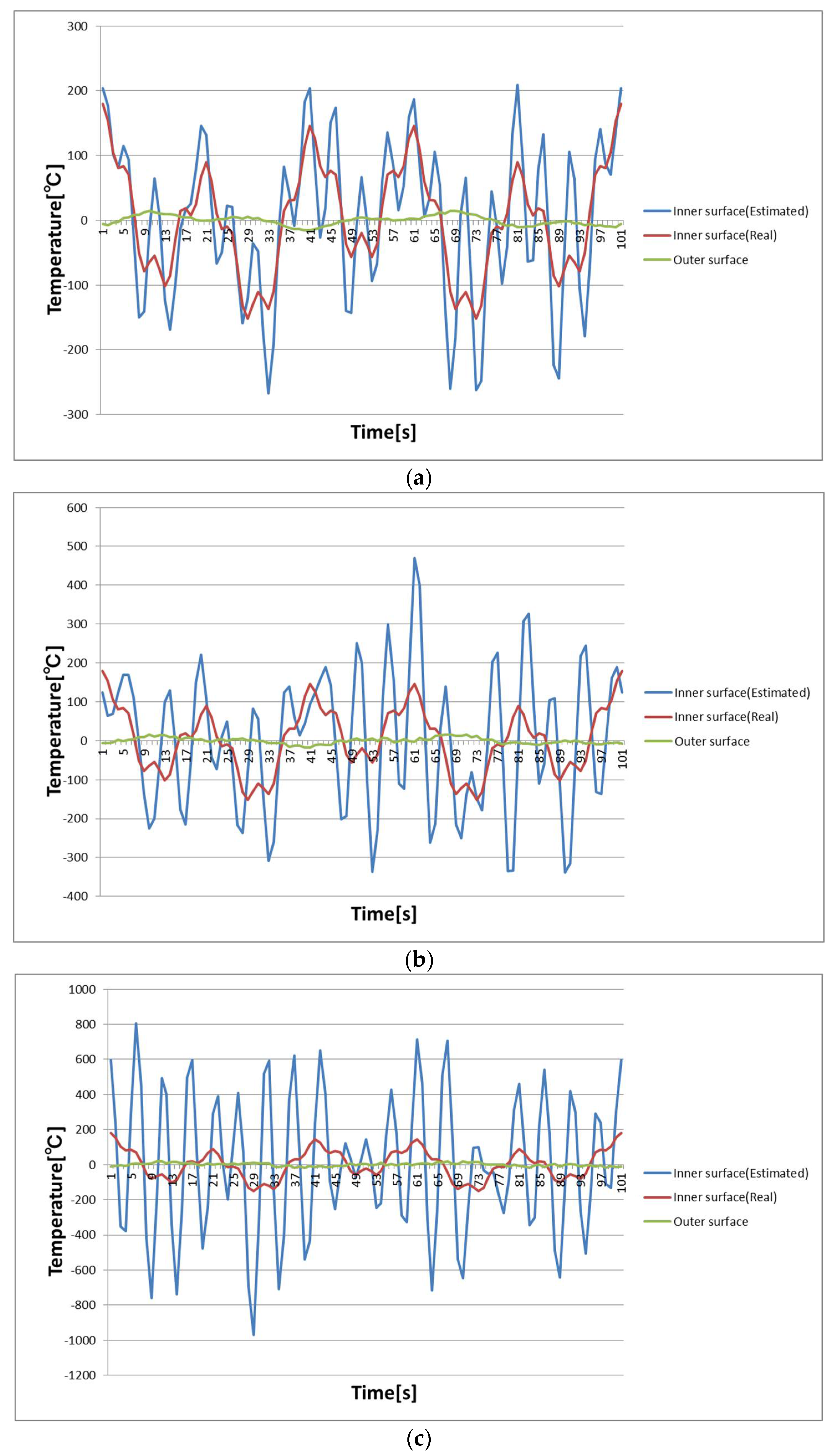
Figure 2.
Estimated temperature variation on inner surface with regulation. (a) Observation noise of 2 °C; (b) Observation noise of 2 °C; (c) Observation noise of 8 °C.
Figure 2.
Estimated temperature variation on inner surface with regulation. (a) Observation noise of 2 °C; (b) Observation noise of 2 °C; (c) Observation noise of 8 °C.

Figure 3.
Thermal stress distribution at t = 5 s.

Table 1.
Amplitude and cycle period of three waves introduced.
| Wave | 1 | 2 | 3 |
|---|---|---|---|
| Amplitude [°C] | 100 | 50 | 30 |
| Cycle Period [s] | 20 | 50 | 5 |
Publisher’s Note: MDPI stays neutral with regard to jurisdictional claims in published maps and institutional affiliations. |
© 2018 by the authors. Licensee MDPI, Basel, Switzerland. This article is an open access article distributed under the terms and conditions of the Creative Commons Attribution (CC BY) license (https://creativecommons.org/licenses/by/4.0/).
Share and Cite
MDPI and ACS Style
Kubo, S.; Taguwa, S. Inverse Analysis for Estimating Temperature and Residual Stress Distributions in a Pipe from Outer Surface Temperature Measurement and Its Regularization. Proceedings 2018, 2, 407. https://doi.org/10.3390/ICEM18-05284
AMA Style
Kubo S, Taguwa S. Inverse Analysis for Estimating Temperature and Residual Stress Distributions in a Pipe from Outer Surface Temperature Measurement and Its Regularization. Proceedings. 2018; 2(8):407. https://doi.org/10.3390/ICEM18-05284
Chicago/Turabian StyleKubo, Shiro, and Shoki Taguwa. 2018. "Inverse Analysis for Estimating Temperature and Residual Stress Distributions in a Pipe from Outer Surface Temperature Measurement and Its Regularization" Proceedings 2, no. 8: 407. https://doi.org/10.3390/ICEM18-05284