Vision-Based Autonomous Landing of a Quadrotor on the Perturbed Deck of an Unmanned Surface Vehicle


Autonomous Marine Systems Research Group, School of Engineering, University of Plymouth, Plymouth PL4 8AA, UK
*
Author to whom correspondence should be addressed.
Drones 2018, 2(2), 15; https://doi.org/10.3390/drones2020015
Submission received: 5 March 2018
/
Revised: 11 April 2018
/
Accepted: 11 April 2018
/
Published: 14 April 2018
Abstract
:Autonomous landing on the deck of an unmanned surface vehicle (USV) is still a major challenge for unmanned aerial vehicles (UAVs). In this paper, a fiducial marker is located on the platform so as to facilitate the task since it is possible to retrieve its six-degrees of freedom relative-pose in an easy way. To compensate interruption in the marker’s observations, an extended Kalman filter (EKF) estimates the current USV’s position with reference to the last known position. Validation experiments have been performed in a simulated environment under various marine conditions. The results confirmed that the EKF provides estimates accurate enough to direct the UAV in proximity of the autonomous vessel such that the marker becomes visible again. Using only the odometry and the inertial measurements for the estimation, this method is found to be applicable even under adverse weather conditions in the absence of the global positioning system.
1. Introduction
In the last few years, significant interest has grown towards unmanned aerial vehicles (UAVs), as described in [1]. The applications involving UAVs range from scientific exploration and data collection [2,3,4], to commercial services, military reconnaissance and law enforcement [5,6], search and rescue [7,8], patrolling [9] and even entertainment [10].
Among different UAVs topologies, helicopter flight capabilities such as hovering or vertical take-off and landing (VTOL) represent a valuable advantage over fixed-wing aircraft. The ability of autonomously landing is very important for unmanned aerial vehicles, and landing on the deck of an un-/manned ship is still an open research area. Landing a UAV on an unmanned surface vehicle (USV) is a complex multi-agent problem [11], and solutions to this can be used for numerous applications such as disaster monitoring [12], coastal surveillance [13,14] and wildlife monitoring [15,16]. In addition, a flying vehicle can also represents an additional sensor data source when planning a safe collision-free path for USVs [17].
Flying a UAV in the marine environment, one encounters rough and unpredictable operating conditions due to the influence of wind or waves in the manoeuvre compared to land. Apart from the above, there are various other challenges associated with the operation of UAVs; for example, the inaccuracy of low-cost GPS units mounted on most UAV and the influence of the electrical noise generated by the motors and on-board computers on magnetometers. In addition to this, the estimation of the USV’s movements is a difficult task due to natural disturbances (e.g., winds, sea currents, etc.). This poses difficulty for a UAV to land on a moving marine vehicle with low quality pose information. To overcome these issues, the camera mounted on the UAV and commonly used during surveillance missions [18] can also be used to increase the accuracy of the relative-pose estimates between the aerial vehicle and the landing platform [19]. The adoption of fiducial markers on the vessel’s deck is proposed as a solution to further improve the estimate results. To increase the robustness of the approach, a state estimation filter is adopted for predicting the six degrees-of-freedom (DOF) pose of the landing deck, which is not perceived by the UAV’s cameras. This work can be considered as the natural consequence of [20], in which the developed algorithm has been tested against a mobile ground robot, without any pitch and roll movements of the landing platform.
In terms of the paper’s organisation, Section 2 presents the method existing in the literature about autonomous landing for UAVs, while Section 3 introduces the quad-copter model, the image processing library used for the deck identification, the UAV controller and the pose estimation filter. In Section 4, three experiments, each with a different kind of perturbation acting on the landing platform, are presented and discussed. Finally, conclusions and future works are shown in Section 5.
2. State of the Art
Autonomous landing has until now been one of the most dangerous challenges for UAV. Inertial navigation systems (INS) and global navigation satellite systems (GNSS) are the traditional sensors of the navigation system. On the other hand, INS accumulates error while integrating position and velocity of the vehicle, and the GNSS sometimes fails when satellites are occluded by buildings. At this stage, vision-based landing became attractive because it is passive and does not require any special equipment other than a camera (generally already mounted on the vehicle) and a processing unit. The problem of accurately landing using vision-based control has been well studied. For a detailed survey about autonomously landing, please refer to [21,22,23]. Here, only a small amount of works is presented.
In [24,25], an IR-LED helipad is adopted for robust tracking and landing, while a more traditional T-shaped and H-shaped helipad are used respectively in [26,27,28,29]. The landing site is searched for an area whose pixels have a contrast value below a given threshold in [30]. In [31], a light imaging, detection and ranging (LIDAR) sensor is combined with a camera, and the approach has been tested with a full-scale helicopter. Bio-inspired by honeybees that use optic flow to guide landing, [32] follow the approach for fixed-wing UAV. The same has been done in [33,34] showing that by maintaining constant optic flow during the manoeuvre, the vehicle can be easily controlled. Hovering and landing control of a UAV on a large textured moving platform enabled by measuring optical flow is achieved in [35]. In [36], a vision algorithm based on multiple view geometry detects a known target and computes the relative position and orientation. The controller is able to control only the x and y positions to hover on the platform. In a similar work [37], the authors were also able to regulate the UAV’s orientation to a set point hover. In [38], an omnidirectional camera has been used to extend the field of view of the observations.
Four light sources have been located on a ground robot, and homography is used to perform autonomous take-off, tracking and landing on a UGV [39]. In order to land on a ground robot, [40] introduces a switching control approach based on optical flow to react when the landing pad is out of the UAV’s camera field of view. In [41], the authors propose the use of an IR camera to track a ship from long distances using its shape, when the ship-deck and rotorcraft are close. Similarly, [42] address the problem of landing on a ship moving only on a 2D plane without its motion known in advance.
The work presented in this paper must be collocated among vision-based methods. Differently from most of them, given the platform used, it relies on a pair of low resolution fixed RGB cameras, without requiring the vehicle to be provided with other sensors. Furthermore, instead of estimating the current pose of the UAV, in order to land on a moving platform, we employ an extended Kalman filter to predict the current position of the vessel on the deck of which the landing pad is located. The estimate is forwarded as input to our control algorithm that updates the last observed USV’s pose and sends a new command to the UAV. In this way, even if the landing pad is no longer within the camera’s field of view, the UAV can start a recovery manoeuvre that, differently from other works, takes the drone in proximity to its final destination. In this way, it can compensate interruptions in the tracking due to changes in attitude of the USV’s deck on which the pad is located.
3. Methods
In this section, all the components used to accomplish the autonomous landing on an USV are introduced. Initially, the aerial vehicle, together with its mathematical formulation, is described. Successively, the ar_pose computer vision library is presented. In the end, the controller and the pose estimation filter are discussed. A graphical representation of these components is depicted in Figure 1, and a video showing the overall working principle is available online (video showing the working principle of the algorithm: https://youtu.be/J1ib9PIsr-8).
3.1. Quad-Copter Model
The quad-copter in this study is an affordable ($250 USD in 2017) AR Drone 2.0 built by the French company Parrot. and it comprises multiple sensors such as two cameras, a processing unit, gyroscope, accelerometers, magnetometer, altimeter and pressure sensor. It is equipped with an external hull for indoor navigation, and it is mainly piloted using smart-phones and tablets through the application released by the producer over a WiFi network. Despite the availability of an official software development kit (SDK), the Robot Operating System (ROS) [43] framework is used to communicate with it, using in particular the ardrone-autonomy package developed by the Autonomy Laboratory of Simon Fraser University and the the tum-ardrone package [44,45,46] developed within the TUM Computer Vision Group in Munich. These packages run within ROS Indigo on a GNU/Linux Ubuntu 14.04 LTS machine. The specifications of the UAV are as follows:
- Dimensions: 53 cm × 52 cm (hull included);
- Weight: 420 g;
- IMU, including gyroscope, accelerometer, magnetometer, altimeter and pressure sensor;
- Front-camera with a high-definition (HD) resolution (1280 × 720), a field of view (FOV) of and video streamed at 30 frames per second (fps);
- Bottom-camera with a Quarted Video graphics Array (QVGA) resolution (320 × 240), a FOV of and video streamed at 60 fps;
- Central processing unit running an embedded version of the Linux operating system;
The downward-looking camera is mainly used to estimate the horizontal velocity, and the accuracy of the estimation highly depends on the ground texture and the quad-copter’s altitude. Only one of the two video streams can be streamed at the same time. Sensors’ data are generated at 200 Hz. The on-board controller (closed-source) is used to act on the roll and pitch , the yaw and the altitude of the platform z. Control commands u = (, ,, z) ∈ [−1,1] are sent to the quad-copter at a frequency of 100 Hz.
While defining the UAV dynamics model, the vehicle must be considered as a rigid body with 6-DOF able to generate the necessary forces and moments for moving [47]. The equations of motion are expressed in the body-fixed reference frame [48]:
where and represent, respectively, the linear and angular velocities of the UAV in . F is the translational force combining gravity, thrust and other components, while is the inertial matrix subject to F and torque vector .
The orientation of the UAV in air is given by a rotation matrix R from to the inertial reference frame :
where is the Euler angles vector and and are abbreviations for and .
Given the transformation from the body frame to the inertial frame , the gravitational force and the translational dynamics in are obtained in the following way:
where g is the gravitational acceleration, is the resulting force in and and are the UAV’s position and velocity in .
3.2. Augmented Reality
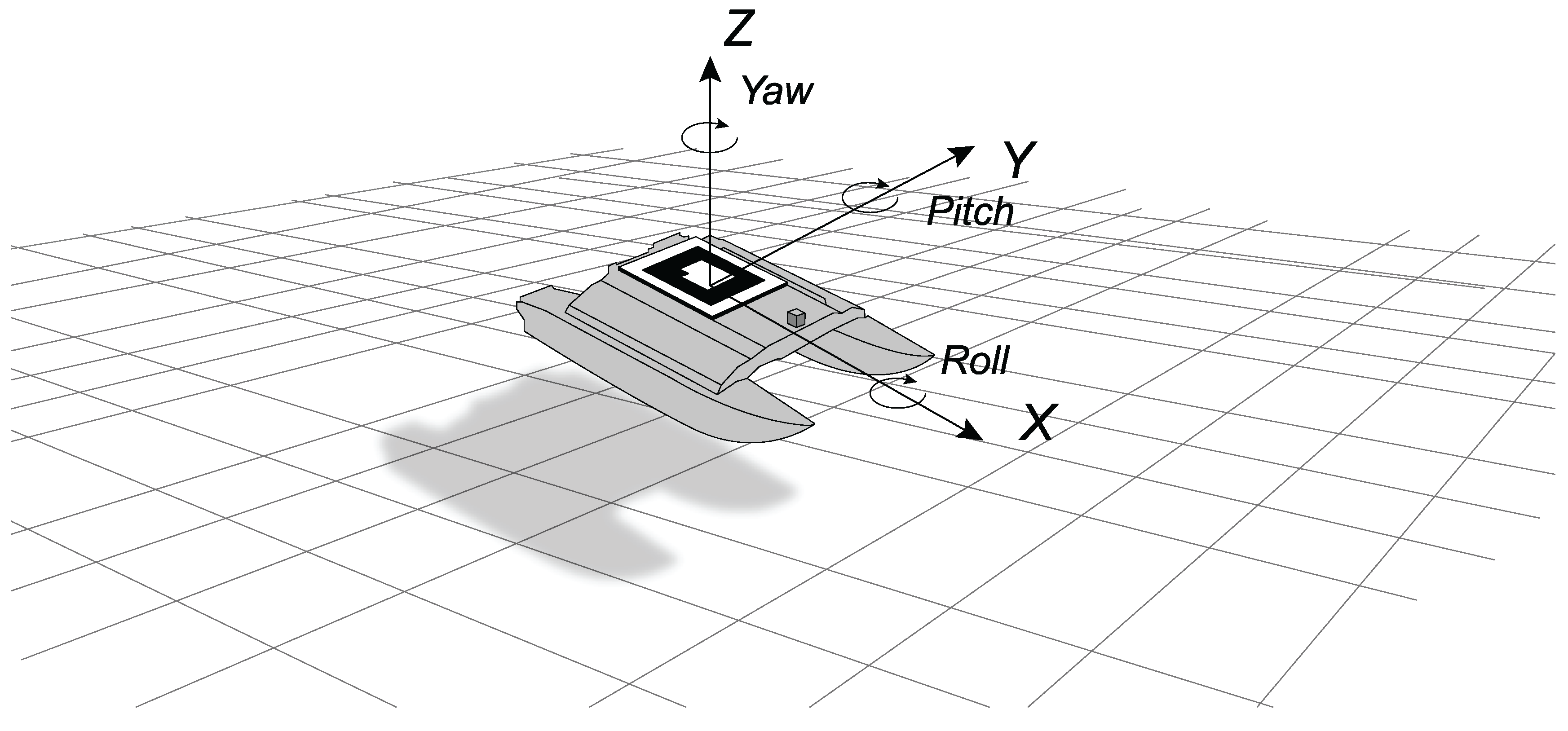
The UAV’s body frame follows the right-handed z-up convention such that the positive x-axis is oriented along the UAV’s forward direction of travel. Both camera frames are fixed with respect to the UAV’s body frame, but translated and rotated in such a way that the positive z-axis points out of the camera lens, the x-axis points to the right from the image centre and the y-axis points down. The USV’s frame also follows the same convention and is positioned at the centre of the landing platform. Finally, a local frame fixed has been defined with respect to the world and initialized by the system at an arbitrary location. In Figure 2, the coordinate systems previously described are depicted.
The pose of frame j with respect to frame i is now defined as the 6-DOF vector:
composed of the translation vector from frame i to frame j and the Euler angles , , .
Then, the homogeneous coordinate transformation from frame j to frame i can be written as:
where is the orthonormal rotation matrix that rotates frame j into frame i and is defined as:
Figure 3 offers a graphical representation of the problem studied: retrieving the homogeneous matrix H offers the possibility to calculate the UAV’s pose with reference to the USV expressed as translation and rotation along and around three axes, respectively.
In this work, augmented reality (AR) visual markers are adopted to identify the landing platform. As described in [49], “in a AR virtual objects super-imposed upon or composited with the real world. Therefore, AR supplements reality”.
The ar_pose ROS package [50], a wrapper for the ARToolkit library widely used in human computer interaction (HCI) [51,52], is used to achieve this task. The ar_pose markers are high-contrast 2D tags designed to be robust to low image resolution, occlusions, rotations and lighting variation. For this reason, it is considered suitable for a possible application in a marine scenario, where the landing platform can be subject to adverse conditions that can affect its direct observation.
In order to use this library, the camera calibration file, the marker’s dimension and the proper topic’s name must be defined inside a configuration file. The package subscribes to one of the two cameras. Pixels in the current frame are clustered based on the similar gradient, and candidate markers are identified. The direct linear transform (DLT) algorithm [53] maps the tag’s coordinate frame to the camera’s frame, and the candidate marker is searched for within a database containing pre-trained markers. The points in the marker’s frame and camera’s frame are respectively denoted as MP and CP. Therefore, the transformation from one frame to the other is defined as follows:
where and represent the transforms from the marker to the camera frame and vice versa, respectively.
Using the camera’s calibration file and the actual size of the marker of interest, the 6-DOF relative-pose of the marker’s frame with respect to the UAV camera is estimated at a frequency of 1 Hz. For the current and the last marker’s observation, the time stamp and the transformation are recorded. This information is then used to detect if the marker has been lost and to actuate a compensatory behaviour.
3.3. Controller
In order to control the drone in a less complex way, the PID controller offered by the tum_ardrone package has been replaced with a (critically) damped spring one.
In the original work of [46], for each of the four degrees of freedom (roll , pitch , the yaw and the altitude ), a separate PID controller is employed. Each of them is used to steer the quad-copter toward a desired goal position in a global coordinate system. The generated controls are then transformed into a robotic-centric coordinate frame and sent to the UAV at 100 Hz.
In this paper, in order to simplify the process of tuning the controller’s parameters, a damped spring controller has been adopted. In the implementation, only two parameters, and , were used to modify the spring strength of the directly controlled dimensions ( and z) and the leaning ones (x and y). An additional one, , is responsible for approximating a damped spring and accounting for external disturbances such as air resistance and wind.
The controller inputs are variations in the angles of roll, pitch, yaw and altitude, respectively denoted as , , and , defined as follows:
where and are the damping coefficients calculated in the following way:
Therefore, instead of controlling nine independent parameters (three for the yaw, three for the vertical speed and three for roll and pitch paired together), the control problem is reduced to the three described above (namely , and ).
The remaining controller parameters are platform-dependent variables, and they are kept always constant during all the trials. Ignoring , which does not require an additional description more than its name, , and limit the rotation and linear speed on the yaw and z-axis, respectively. In the end, limits the maximum leaning command sent.
The controller’s parameters are the same across all the experiments performed, and they are shown in Table 1. The parameter, responsible for controlling the roll and pitch behaviour, is kept small in order to guarantee smooth movements along the leaning dimensions. In the same way, has been reduced to a value of to decrease the descending velocity. On the other hand, the parameter, used to control the yaw speed, has been set to its maximum value because the drone must align with the base in the minimum amount of time possible. The others have been left at their default values.
3.4. Pose Estimation
To increase the robustness and efficiency of the approach, an extended Kalman filter (EKF) has been adopted here to estimate the pose of the landing platform [54]. In fact, it may happen that the UAV loses track of the fiducial marker while approaching and descending on it. In order to redirect the flying vehicle in the right direction, the EKF estimates the USV’s current pose, which is then processed and forwarded to the controller. For estimation purposes, the odometry and inertial data are fused together to increase the accuracy [55,56]. The state vector is defined as , with and representing respectively the global positions and velocity and and the attitude of the vessel. Considering the sensor readings, the estimation process satisfies the following equations:
where k represents a discrete time instant, is a kinematic constant velocity model, is the observation model, is the measurements vector, is an identity matrix, is the process covariance matrix and is the measurement covariance matrix.
The working principle of the EKF in this case is detailed below:
- the filter estimates the USV’s pose at 50 Hz, and its encoding is saved in a hash table using the time stamp as the key;
- when the UAV loses the track, the hash table is accessed, and the last record inserted (the most recent estimate produced by the filter) together with the one having as the key the time stamp of the last recorded observation are retrieved;
- the deck’s current position with reference to the old one is calculated using the geometric relationship;
- the controller commands are updated including the new relative position.
The procedure described above is iterated until the UAV is redirected above the visual marker and can perceive it through its bottom camera.
3.5. Methodology
The following section explains how the Algorithm 1 works. The code is publicly available on our repository (Github repository: https://github.com/pulver22/ardrone_tf_controller).
| Algorithm 1 Landing Algorithm. |
|
The quad-copter flies using its fixed non-tilting frontal camera, approaching the landing site on the USV’s deck identified only by a fiducial marker. This, the scope of which is to outline the landing area, has to be perceived during the entirety of the landing manoeuvre. This is a requirement for precise landing despite the state estimator being able to compensate an interruption in observation. When a visual marker is detected, the image processing library computes the 6-DOF relative-pose between the marker itself and the UAV. The result is used to make the quad-copter approach the marker with the right orientation. To obtain this result, a damped spring controller reduces the error on the x-, y- and z-axis and on the quad-copter’s . On attaining close proximity to the marker, the marker leaves the field of view of the frontal camera. This is due to hardware limitation of fixed non-tilting cameras. To overcome this problem, the video stream from the frontal camera is interrupted and acquired from the one located under the UAV and downward-looking. The quad-copter continues the landing manoeuvre keeping the marker at the centre of the second camera’s FOV. Otherwise, a compensatory behaviour is adopted: the EKF estimates the actual position of the USV, and the drone is redirected close to it while increasing its altitude. Increasing the altitude allows enlarging the field of view of the bottom camera, which is quite limited. In this way, it is guaranteed that the marker will soon be perceived and centred by the aerial vehicle. When an experimentally-defined distance from the marker is reached, the drone lands safely. This distance depends on the side length of the marker used. In fact, with a smaller marker, it would be possible to decrease this value, but it would become impossible to perceive the marker at a longer distance. We found that a marker side length of approximately 0.30 m represents a good trade-off for making the marker visible at a long and a close distance at the same time. As a consequence, we decide to use 0.75 m as the distance for starting the touchdown phase of the descending manoeuvre, during which the power of the motors is progressively reduced until complete shut-down. The use of visual markers allows the estimation of the full 6-DOF pose information of the aerial and surface vehicles. In this way, landing operations in a rough sea condition with a significant pitching and rolling deck can still be addressed.
4. Results and Discussion
All the experiments have been conducted inside a simulated environment built on Gazebo 2.2.X and offering a 3D model of the AR Drone 2.0. In the scope of this work, the existing simulator has been partially rewritten and extended to support multiple different robots at the same time. The Kingfisher USV, produced by Clearpath Robotics, has been used as the floating base. It is a small catamaran with dimensions of 135 × 98 cm, which can be deployed in an autonomous or teleoperated way. It is equipped with a flat plane representing a versatile deck for UAVs of small dimensions. On this surface, a square visual marker is placed. Previous research demonstrated that a linear relationship exists between the side length of the marker and its observability. Therefore, we opted for a side length of 0.3 m, which represents a good compromise, making the marker visible in the range [0.5, 6.5] meters.
The algorithm has been tested under multiple conditions, namely three. In the first scenario, the USV is subjected only to a rolling movement, while floating in the same position for the entire length of the experiment; in the second scenario, the USV is subjected only to a pitching movement; while in the last scenario, the USV is subject to both rolling and pitching disturbances at the same time. Figure 4 illustrates the rotation angles around their corresponding axis. In all the simulations, the disturbances are modelled as a signal having a maximum amplitude of five degrees and a frequency of 0.2 Hz. Rolling and pitching of a vessel generate upward and downward acceleration forces directed tangentially to the direction of rotation, which cause linear motion known as swaying and surging along the transverse or longitudinal axis, respectively [57].
4.1. Rolling Platform
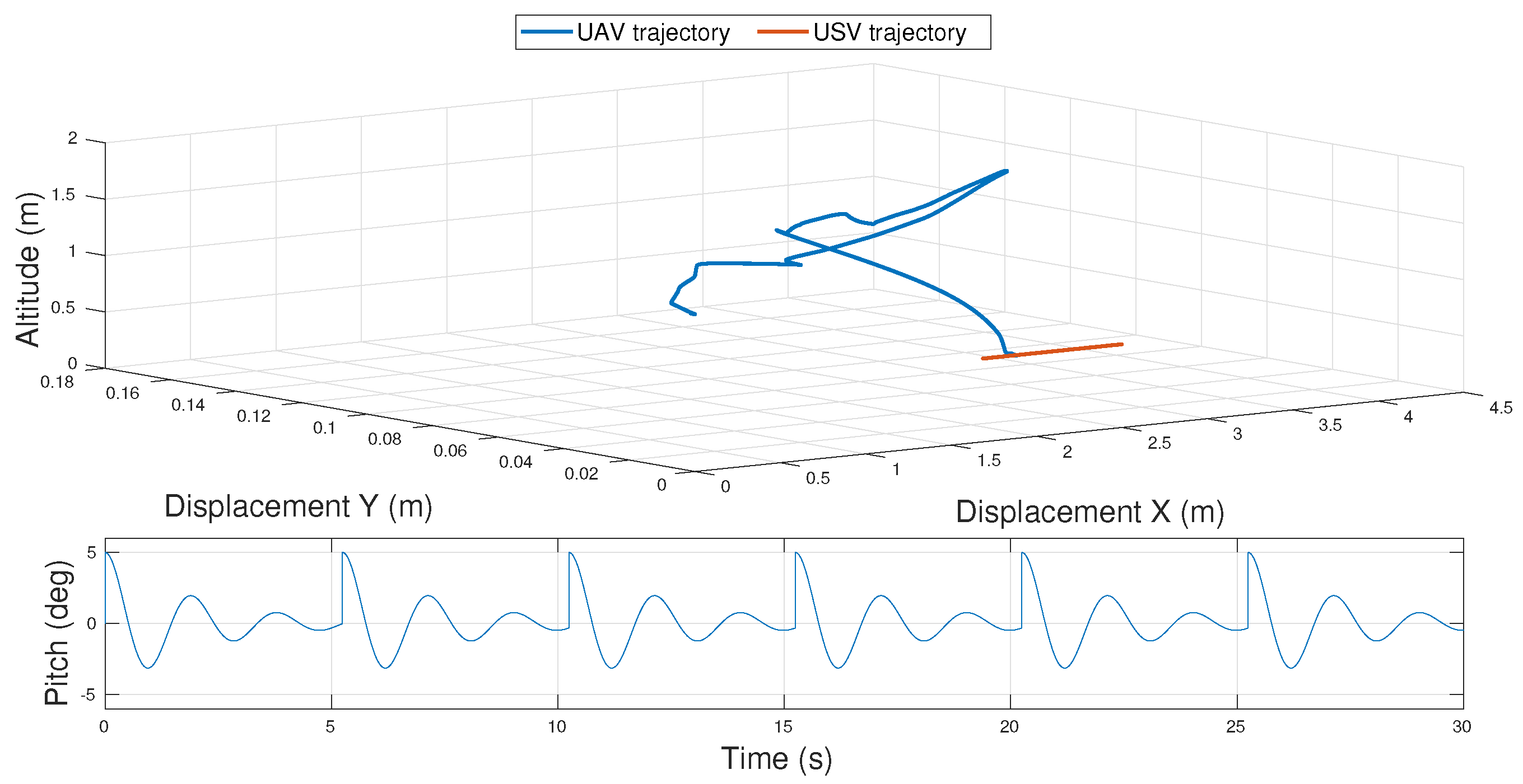
In this subsection, the results of a landing manoeuvre on a rolling floating base are reported. In particular, Figure 5 illustrates the UAV’ and the USV’s trajectory, respectively in blue and red, in the UAV’s reference frame; while Figure 6 and Figure 7 show the controller commands and the salient moments of the manoeuvre, respectively.
The marker has been successfully recognised at a distance of 3.74 m in front of the UAV and at 0.09 m to its left. The displacement on the z-axis, used as a reference for the altitude, was of 0.84 m instead. The UAV, with the parameters reported in the previous Table 1, was able to complete the landing in 25 s.
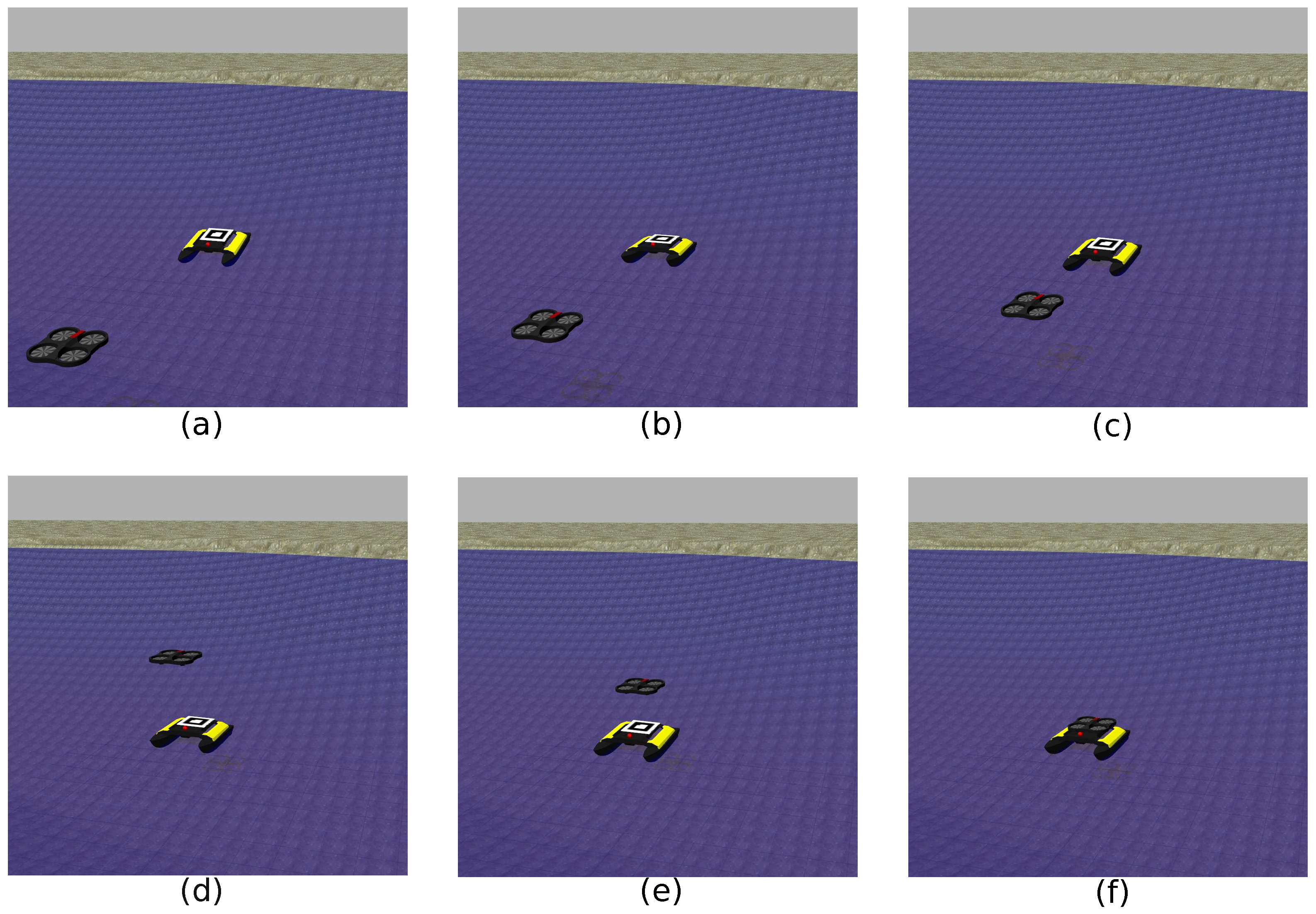
The quad-copter approaches the landing base trying to keep it at the centre (in a range of ±10 degrees) of its camera’s FOV. In the case that the marker leaves this interval of tolerance, the UAV would rotate around its z-axis in order to centre it again. The approach continues until the UAV’s low altitude prevents the marker from being seen by the frontal camera, as shown in Figure 7a ( s). At this point, the video stream is switched from the frontal camera to the one located at the bottom of the quad-copter and looking down, and new commands are generated and sent. The UAV is instructed to move towards the last known position of the landing platform, but increasing its altitude in order to enlarge the area covered by its bottom camera. At s, as represented in Figure 7b, the UAV is located exactly above the marker, and it can now complete the landing phase: it descends while trying to keep the marker at the centre of its FOV, as shown in Figure 7c. Small velocity commands are sent on the leaning direction (x and y, respectively) in order to approach the final position with high accuracy. Finally, at s, the UAV reaches the minimum altitude required to shut-down its motors and land on the platform (Figure 7f).
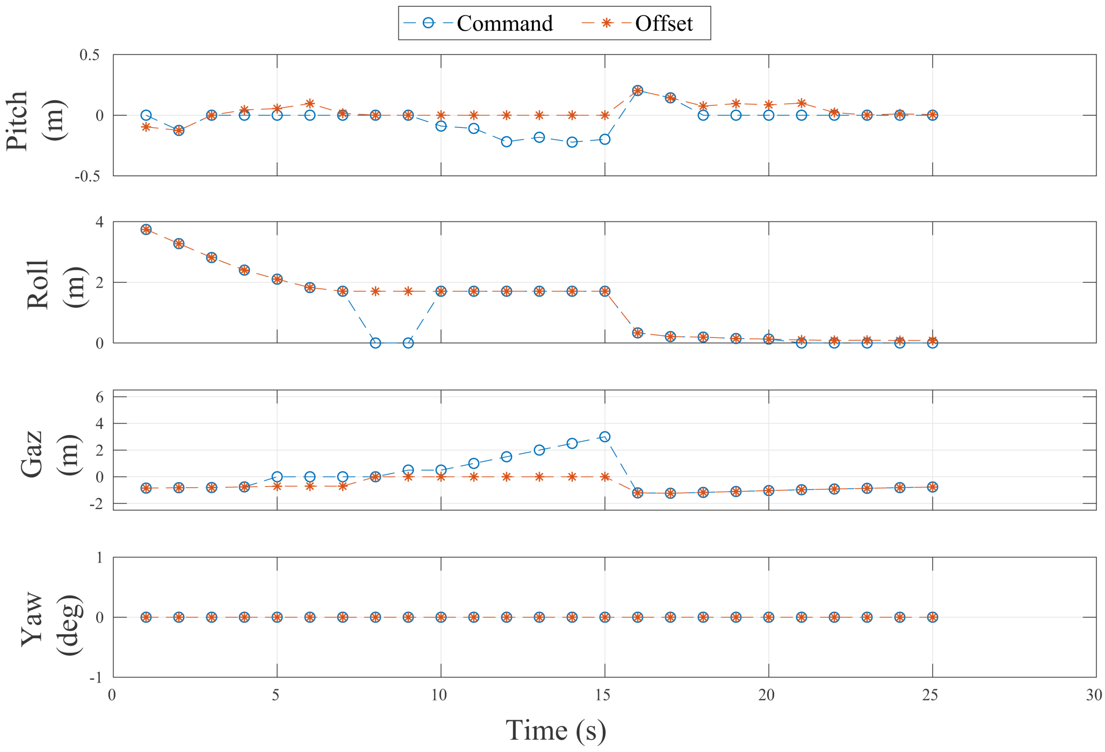
The commands generated from the relative-pose between the UAV and the landing platform’s frame are illustrated in Figure 5. Here, the controller’s commands are plotted against the perception from the camera. As is possible to see in the figure, for most of the travel, the two curves of the commands and of the observations overlap perfectly. When they do not, the marker is lost, and the UAV actuates the compensatory behaviour: the estimation filter’s output, namely the USV’s predicted pose, is combined with the latest visual observation in order to generate new commands for the UAV. In this way, it is possible to explain the change in roll, pitch and altitude in the graph. Since the UAV has the same yaw of the floating base, namely they have the same orientation along the z-axis, no rotation commands are issued for this degree of freedom.
A few words are reserved for the pitch’s data between s and s and the gaz’s data between s and s. In this case, the offsets are below a user-defined threshold, and a null command is sent instead. The use of a threshold has been introduced for speeding up the landing phase: while testing the controller, it was noticed that the UAV spent much time trying to align perfectly on the three axes with the centre of the landing plane, sometimes without any success. This has been identified as a limitation of controllers with fixed value parameters, and a new, more versatile solution is already planned as future work.
4.2. Pitching Platform
In this subsection, an experiment with a pitching floating platform is reported. As before, the time for completing the landing manoeuvre is not considered as a key factor, but the attention is on the ability of the UAV to approach and land on the USV with high precision.
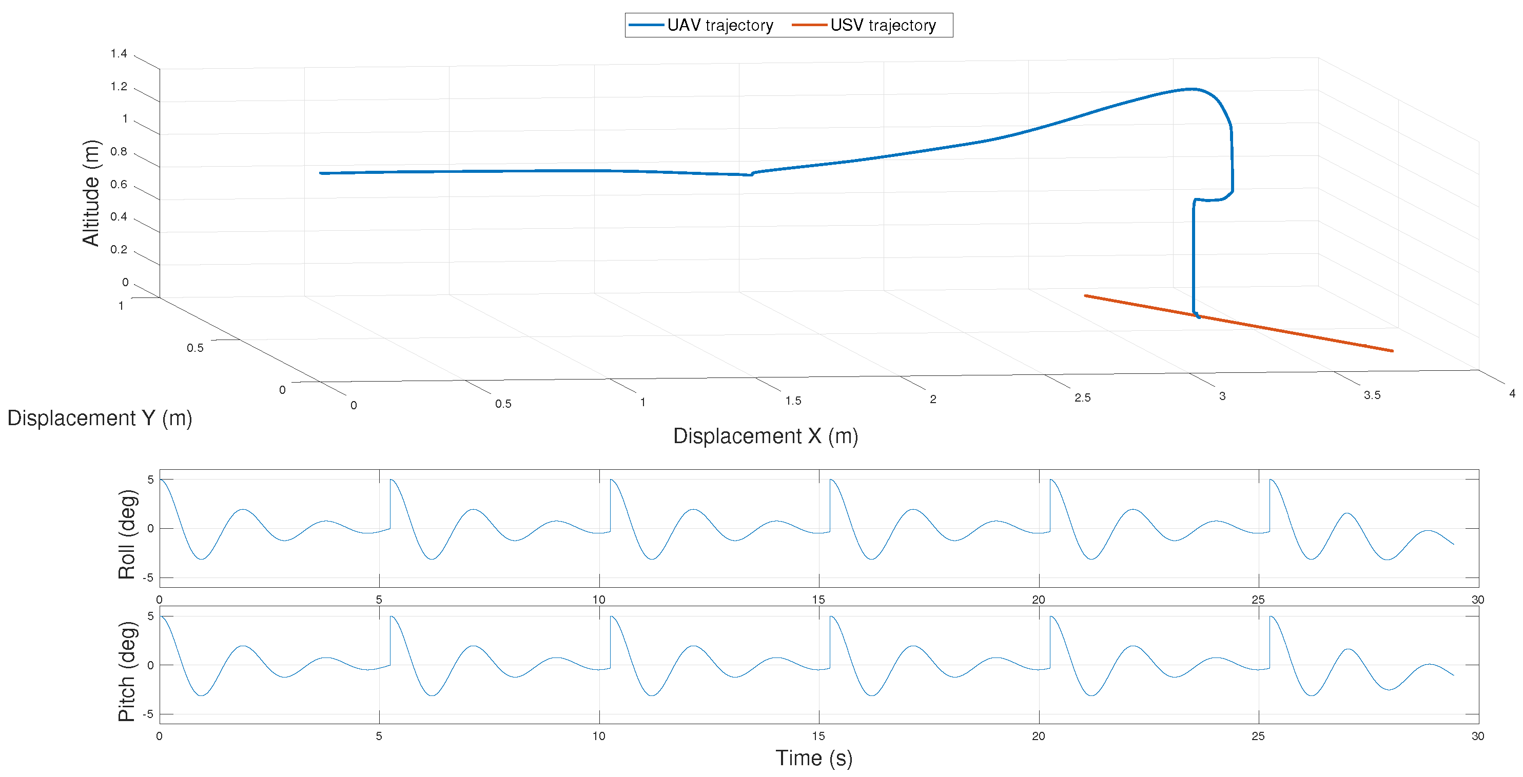
As in the previous experiments, the two vehicles’ 3D trajectories are reported in Figure 8 in the UAV’s reference frame, the controller commands in Figure 9 and example frames in Figure 10. The quad-copter, with the same controller parameters as before, was able to follow and land on the visual marker in almost 34 s after identifying it 4.46 m ahead and 0.12 m on its left.
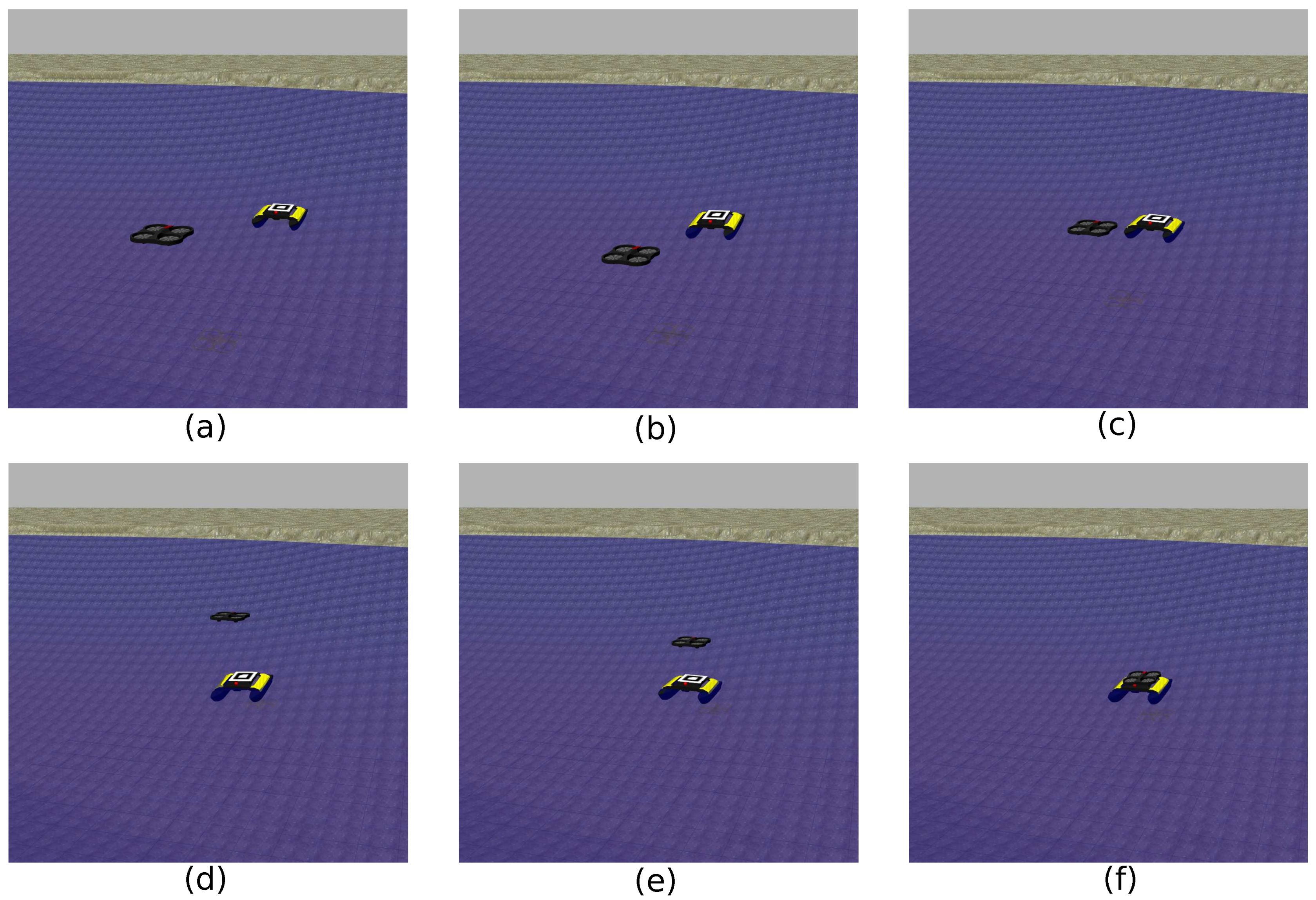
As in the case of a rolling base, Figure 10a shows that the UAV starts moving in order to keep the visual marker at the centre of its frontal camera’s field of view. This is what happens at time s and shown in Figure 10b. At s, the UAV reaches its minimum altitude, and it is now impossible for it to see the visual marker, as illustrated in Figure 10c. At this point, the video stream starts to be acquired from the bottom camera, and the USV’s estimated position is sent to the controller; at the same time, instructing the UAV to increase its altitude to augment the total area covered with its downward-looking camera. Doing this, at s, the UAV is located exactly above the USV. The landing base is at the centre of the camera’s FOV; therefore, a null velocity command is sent to stop the USV. Figure 10e,f shows that the UAV can then descend slowly to centre the marker properly and, in the end, land on it.
Further analysis can be done with the results reported in Figure 9. In the same way as the experiment with a rolling deck, the curve of the controller’s commands and the one related to the offsets overlap for most of the time. All the considerations made before still hold: while the marker is lost, the EKF is able to estimate the landing platform’s current pose with reference to the instant of time when the marker has been lost. This relative-pose is added to the last observation in order to produce a new command.
This is what is possible to see in the plot between s and s. Here, the two curves differ: while all the offsets remain constant because no new marker observations have been done by the UAV, the commands (gaz and roll) slightly change. The plot is now discussed in more details. While the yaw and the pitch commands remain identical to zero because the UAV is already aligned with the landing base (within the predefined bounds), the UAV’s roll command is changed including at every instant the new relative-pose (changing in the longitudinal direction) of the USV.
4.3. Rolling and Pitching Platform
The last simulation has been done with a floating platform that is subject to both rolling and pitching stresses. The goal of this experiment is to test the developed landing algorithm against simulated harsh marine conditions.
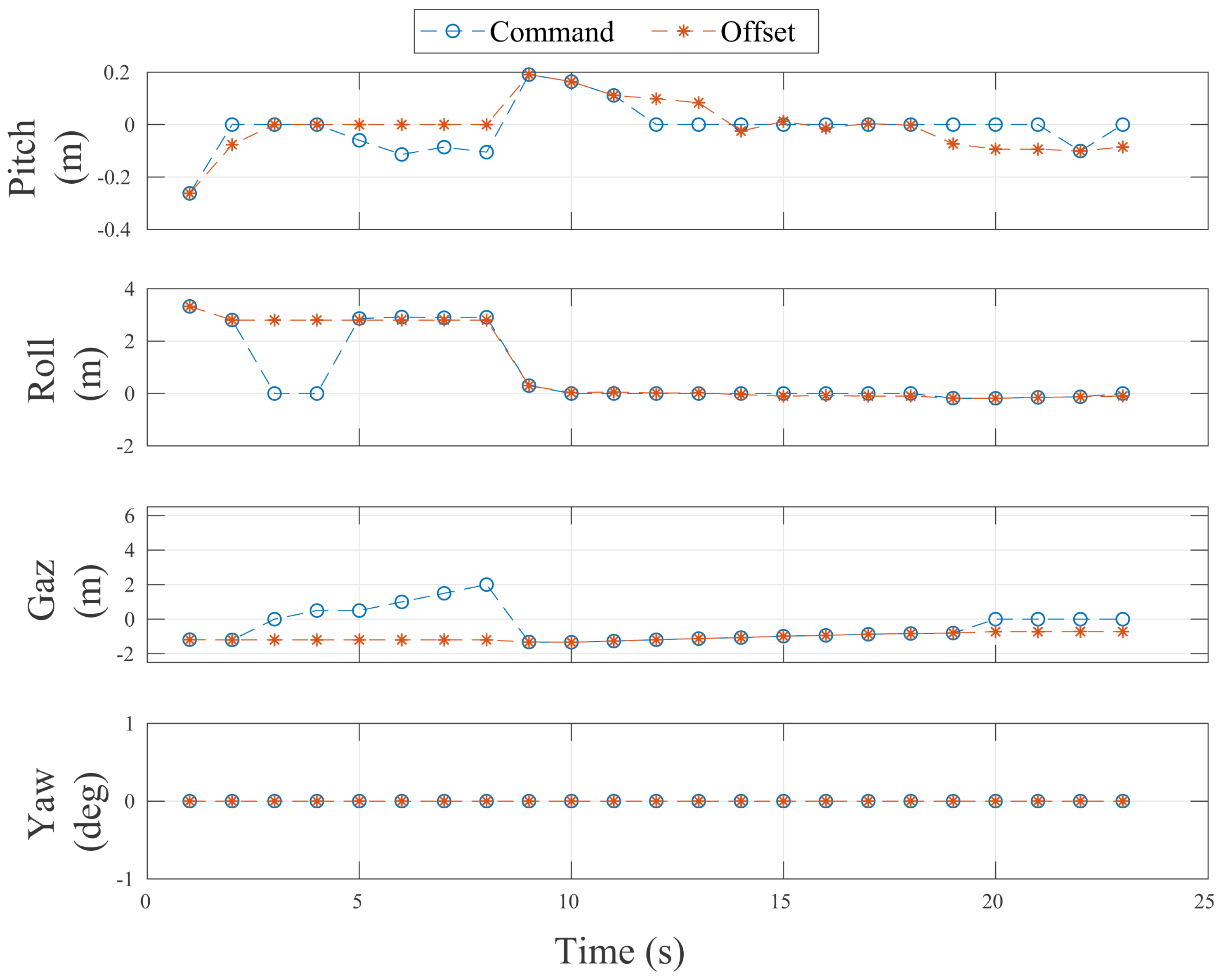
The results are reported in Figure 11, showing both vehicles trajectories along a 23-s operation. The UAV successfully accomplishes the landing manoeuvre starting from an initial marker’s identification 3.71 m in front of it and 0.30 m to its left. Figure 12 shows the comparison between the offsets obtained through the vision algorithm and the commands sent to the controller. It is possible to see that, as in the previous experiments, the curve of the offsets and the one related to the commands mainly overlap. All the analyses made before are still valid, but it is interesting to notice how the framework proposed is able to react properly also when the landing platform is subject to complex disturbances. The salient moments of the flight are illustrated in Figure 13.
5. Conclusions and Future Directions
In this paper, a solution to make an unmanned aerial vehicle autonomously land on the deck of a USV is presented. It relies only on the UAV’s on-board sensors and on the adoption of a visual marker on the landing platform. In this way, the UAV can estimate the 6-DOF landing area position through an image processing algorithm. The adoption of a pose estimation filter (in this case, an extended Kalman filter) allows overcoming issues with fixed non-tilting cameras and the image processing algorithm. Not involving GPS signals in the pose estimation and in the generation of flight commands allows the UAV to land also in situations where this signal is not available (indoor scenarios or adverse weather conditions).
The validation of the approach has been done in a simulation with a quad-rotor and an unmanned surface vehicle as the platform on which to land. Three different experiments were performed, each of them with a different type of disturbance acting on the landing base. In all scenarios, successful results were obtained.
The future research is two-fold. From a practical point of view, the proposed approach needs to be tested in a real environment with an unmanned surface vehicle in order to test its robustness against real wind and sea currents. The second aspect is more related to the identified limitation of the algorithm itself. Therefore, it is suggested to develop an adaptive controller, possibly based on an intelligent solution such as artificial neural networks or fuzzy logic, where the gain of the controller change depends on the distance to the landing base.
Author Contributions
Riccardo Polvara wrote the paper, developed the software and conducted all the experiments. Sanjay Sharma and Jian Wan provided valuable feedback and revisions. Andrew Manning and Robert Sutton contributed to writing and proofreading the manuscript.
Conflicts of Interest
The authors declare no conflict of interest.
References
- Kumar, V.; Michael, N. Opportunities and challenges with autonomous micro aerial vehicles. Int. J. Robot. Res. 2012, 31, 1279–1291. [Google Scholar] [CrossRef]
- Shim, D.; Chung, H.; Kim, H.J.; Sastry, S. Autonomous exploration in unknown urban environments for unmanned aerial vehicles. In Proceedings of the AIAA Guidance, Navigation, and Control Conference and Exhibit, San Francisco, CA, USA, 15–18 August 2005; pp. 1–8. [Google Scholar]
- Bourgault, F.; Göktogan, A.; Furukawa, T.; Durrant-Whyte, H.F. Coordinated search for a lost target in a Bayesian world. Adv. Robot. 2004, 18, 979–1000. [Google Scholar] [CrossRef]
- Neumann, P.P.; Bennetts, V.H.; Lilienthal, A.J.; Bartholmai, M.; Schiller, J.H. Gas source localization with a micro-drone using bio-inspired and particle filter-based algorithms. Adv. Robot. 2013, 27, 725–738. [Google Scholar] [CrossRef]
- Murphy, D.W.; Cycon, J. Applications for mini VTOL UAV for law enforcement. In Enabling Technologies for Law Enforcement and Security; International Society for Optics and Photonics: Bellingham, WA, USA, 1999; pp. 35–43. [Google Scholar]
- Colorado, J.; Perez, M.; Mondragon, I.; Mendez, D.; Parra, C.; Devia, C.; Martinez-Moritz, J.; Neira, L. An integrated aerial system for landmine detection: SDR-based Ground Penetrating Radar onboard an autonomous drone. Adv. Robot. 2017, 31, 791–808. [Google Scholar] [CrossRef]
- Tomic, T.; Schmid, K.; Lutz, P.; Domel, A.; Kassecker, M.; Mair, E.; Grixa, I.L.; Ruess, F.; Suppa, M.; Burschka, D. Toward a fully autonomous UAV: Research platform for indoor and outdoor urban search and rescue. IEEE Robot. Autom. Mag. 2012, 19, 46–56. [Google Scholar] [CrossRef]
- Kruijff, G.; Kruijff-Korbayová, I.; Keshavdas, S.; Larochelle, B.; Janíček, M.; Colas, F.; Liu, M.; Pomerleau, F.; Siegwart, R.; Neerincx, M.; et al. Designing, developing, and deploying systems to support human–robot teams in disaster response. Adv. Robot. 2014, 28, 1547–1570. [Google Scholar] [CrossRef]
- Minaeian, S.; Liu, J.; Son, Y.J. Vision-based target detection and localization via a team of cooperative UAV and UGVs. IEEE Trans. Syst. Man Cybern. Syst. 2016, 46, 1005–1016. [Google Scholar] [CrossRef]
- Kim, S.J.; Jeong, Y.; Park, S.; Ryu, K.; Oh, G. A Survey of Drone use for Entertainment and AVR (Augmented and Virtual Reality). In Augmented Reality and Virtual Reality; Springer: Berlin, Germany, 2018; pp. 339–352. [Google Scholar]
- Polvara, R.; Sharma, S.; Sutton, R.; Wan, J.; Manning, A. Toward a Multi-agent System for Marine Observation. In Advances in Cooperative Robotics; World Scientific: Singapore, 2017; pp. 225–232. [Google Scholar]
- Murphy, R.R.; Steimle, E.; Griffin, C.; Cullins, C.; Hall, M.; Pratt, K. Cooperative use of unmanned sea surface and micro aerial vehicles at Hurricane Wilma. J. Field Robot. 2008, 25, 164–180. [Google Scholar] [CrossRef]
- Pereira, E.; Bencatel, R.; Correia, J.; Félix, L.; Gonçalves, G.; Morgado, J.; Sousa, J. Unmanned air vehicles for coastal and environmental research. J. Coast. Res. 2009, 1557–1561. [Google Scholar]
- Pinto, E.; Santana, P.; Barata, J. On collaborative aerial and surface robots for environmental monitoring of water bodies. In Proceedings of the Doctoral Conference on Computing, Electrical and Industrial Systems, Costa de Caparica, Portugal, 15–17 April 2013; pp. 183–191. [Google Scholar]
- Linchant, J.; Lisein, J.; Semeki, J.; Lejeune, P.; Vermeulen, C. Are unmanned aircraft systems (UASs) the future of wildlife monitoring? A review of accomplishments and challenges. Mammal Rev. 2015, 45, 239–252. [Google Scholar] [CrossRef]
- Watts, A.C.; Ambrosia, V.G.; Hinkley, E.A. Unmanned aircraft systems in remote sensing and scientific research: Classification and considerations of use. Remote Sens. 2012, 4, 1671–1692. [Google Scholar] [CrossRef]
- Polvara, R.; Sharma, S.; Wan, J.; Manning, A.; Sutton, R. Obstacle Avoidance Approaches for Autonomous Navigation of Unmanned Surface Vehicles. J. Navig. 2017, 71, 241–256. [Google Scholar] [CrossRef]
- Stacy, N.; Craig, D.; Staromlynska, J.; Smith, R. The Global Hawk UAV Australian deployment: imaging radar sensor modifications and employment for maritime surveillance. In Proceedings of the 2002 IEEE International on Geoscience and Remote Sensing Symposium, Toronto, ON, Canada, 24–28 June 2002; Volume 2, pp. 699–701. [Google Scholar]
- Ettinger, S.M.; Nechyba, M.C.; Ifju, P.G.; Waszak, M. Vision-guided flight stability and control for micro air vehicles. Adv. Robot. 2003, 17, 617–640. [Google Scholar] [CrossRef]
- Polvara, R.; Sharma, S.; Wan, J.; Manning, A.; Sutton, R. Towards Autonomous Landing on a Moving Vessel through Fiducial Markers. In Proceedings of the IEEE European Conference on Mobile Robotics (ECMR), Paris, France, 6–8 September 2017; pp. 1–6. [Google Scholar]
- Kong, W.; Zhou, D.; Zhang, D.; Zhang, J. Vision-based autonomous landing system for unmanned aerial vehicle: A survey. In Proceedings of the 2014 International Conference on Multisensor Fusion and Information Integration for Intelligent Systems (MFI), Beijing, China, 28–29 September 2014; pp. 1–8. [Google Scholar]
- Kendoul, F. Survey of advances in guidance, navigation, and control of unmanned rotorcraft systems. J. Field Robot. 2012, 29, 315–378. [Google Scholar] [CrossRef]
- Sanz, D.; Valente, J.; del Cerro, J.; Colorado, J.; Barrientos, A. Safe operation of mini UAVs: A review of regulation and best practices. Adv. Robot. 2015, 29, 1221–1233. [Google Scholar] [CrossRef]
- Masselli, A.; Yang, S.; Wenzel, K.E.; Zell, A. A cross-platform comparison of visual marker based approaches for autonomous flight of quadrocopters. In Proceedings of the 2013 International Conference on Unmanned Aircraft Systems (ICUAS), Atlanta, GA, USA, 28–31 May 2013; pp. 685–693. [Google Scholar]
- Wenzel, K.E.; Rosset, P.; Zell, A. Low-cost visual tracking of a landing place and hovering flight control with a microcontroller. In Proceedings of the Selected Papers from the 2nd International Symposium on UAVs, Reno, NV, USA, 8–10 June 2009; pp. 297–311. [Google Scholar]
- Cesetti, A.; Frontoni, E.; Mancini, A.; Zingaretti, P.; Longhi, S. A vision-based guidance system for UAV navigation and safe landing using natural landmarks. In Proceedings of the Selected Papers from the 2nd International Symposium on UAVs, Reno, NV, USA, 8–10 June 2009; pp. 233–257. [Google Scholar]
- Yang, S.; Scherer, S.A.; Zell, A. An onboard monocular vision system for autonomous takeoff, hovering and landing of a micro aerial vehicle. J. Intell. Robot. Syst. 2013, 69, 499–511. [Google Scholar] [CrossRef]
- Saripalli, S.; Montgomery, J.F.; Sukhatme, G.S. Visually guided landing of an unmanned aerial vehicle. IEEE Trans. Robot. Autom. 2003, 19, 371–380. [Google Scholar] [CrossRef]
- Hrabar, S.; Sukhatme, G.S. Omnidirectional vision for an autonomous helicopter. In Proceedings of the 2003 IEEE International Conference on Robotics and Automation, Taipei, Taiwan, 14–19 September 2003; Volume 1, pp. 558–563. [Google Scholar]
- Garcia-Pardo, P.J.; Sukhatme, G.S.; Montgomery, J.F. Towards vision-based safe landing for an autonomous helicopter. Robot. Auton. Syst. 2002, 38, 19–29. [Google Scholar] [CrossRef]
- Scherer, S.; Chamberlain, L.; Singh, S. Autonomous landing at unprepared sites by a full-scale helicopter. Robot. Auton. Syst. 2012, 60, 1545–1562. [Google Scholar] [CrossRef]
- Barber, B.; McLain, T.; Edwards, B. Vision-based landing of fixed-wing miniature air vehicles. J. Aerosp. Comput. Inf. Commun. 2009, 6, 207–226. [Google Scholar] [CrossRef]
- Chahl, J.S.; Srinivasan, M.V.; Zhang, S.W. Landing strategies in honeybees and applications to uninhabited airborne vehicles. Int. J. Robot. Res. 2004, 23, 101–110. [Google Scholar] [CrossRef]
- Ruffier, F.; Franceschini, N. Optic flow regulation in unsteady environments: A tethered mav achieves terrain following and targeted landing over a moving platform. J. Intell. Robot. Syst. 2015, 79, 275–293. [Google Scholar] [CrossRef]
- Herissé, B.; Hamel, T.; Mahony, R.; Russotto, F.X. Landing a VTOL unmanned aerial vehicle on a moving platform using optical flow. IEEE Trans. Robot. 2012, 28, 77–89. [Google Scholar] [CrossRef]
- Shakernia, O.; Vidal, R.; Sharp, C.S.; Ma, Y.; Sastry, S. Multiple view motion estimation and control for landing an unmanned aerial vehicle. In Proceedings of the 2002 IEEE International Conference on Robotics and Automation, Washington, DC, USA, 11–15 May 2002; Volume 3, pp. 2793–2798. [Google Scholar]
- Saripalli, S.; Montgomery, J.F.; Sukhatme, G.S. Vision-based autonomous landing of an unmanned aerial vehicle. In Proceedings of the 2002 IEEE International Conference on Robotics and Automation, Washington, DC, USA, 11–15 May 2002; Volume 3, pp. 2799–2804. [Google Scholar]
- Kim, J.; Jung, Y.; Lee, D.; Shim, D.H. Outdoor autonomous landing on a moving platform for quadrotors using an omnidirectional camera. In Proceedings of the 2014 International Conference on Unmanned Aircraft Systems (ICUAS), Orlando, FL, USA, 27–30 May 2014; pp. 1243–1252. [Google Scholar]
- Wenzel, K.E.; Masselli, A.; Zell, A. Automatic take off, tracking and landing of a miniature UAV on a moving carrier vehicle. J. Intell. Robot. Syst. 2011, 61, 221–238. [Google Scholar] [CrossRef]
- Gomez-Balderas, J.E.; Flores, G.; Carrillo, L.G.; Lozano, R. Tracking a ground moving target with a quadrotor using switching control. J. Intell. Robot. Syst. 2013, 70, 65–78. [Google Scholar] [CrossRef] [Green Version]
- Yakimenko, O.A.; Kaminer, I.I.; Lentz, W.J.; Ghyzel, P. Unmanned aircraft navigation for shipboard landing using infrared vision. IEEE Trans. Aerosp. Electron. Syst. 2002, 38, 1181–1200. [Google Scholar] [CrossRef]
- Belkhouche, F. Autonomous Navigation of an Unmanned Air Vehicle Towards a Moving Ship. Adv. Robot. 2008, 22, 361–379. [Google Scholar] [CrossRef]
- Quigley, M.; Conley, K.; Gerkey, B.; Faust, J.; Foote, T.; Leibs, J.; Wheeler, R.; Ng, A.Y. ROS: An open-source Robot Operating System. In Proceedings of the ICRA workshop on open source software, Kobe, Japan, 12 May 2009; Volume 3, p. 5. [Google Scholar]
- Engel, J.; Sturm, J.; Cremers, D. Accurate figure flying with a quadrocopter using onboard visual and inertial sensing. Imu 2012, 320, 240. [Google Scholar]
- Engel, J.; Sturm, J.; Cremers, D. Camera-based navigation of a low-cost quadrocopter. In Proceedings of the 2012 IEEE/RSJ International Conference on Intelligent Robots and Systems, Vilamoura, Portugal, 7–12 October 2012; pp. 2815–2821. [Google Scholar]
- Engel, J.; Sturm, J.; Cremers, D. Scale-Aware Navigation of a Low-Cost Quadrocopter with a Monocular Camera. Robot. Auton. Syst. 2014, 62, 1646–1656. [Google Scholar] [CrossRef]
- Nonami, K.; Kendoul, F.; Suzuki, S.; Wang, W.; Nakazawa, D. Autonomous Flying Robots: Unmanned Aerial Vehicles and Micro Aerial Vehicles, 1st ed.; Springer Publishing Company: New York, NY, USA, 2010. [Google Scholar]
- Goldstein, H. Classical Mechanics; World Student Series; Addison-Wesley: Boston, MA, USA; Reading, MA, USA; Menlo Park, CA, USA; Amsterdam, The Netherlands, 1980. [Google Scholar]
- Azuma, R.T. A survey of augmented reality. Presence Teleoperators Virtual Environ. 1997, 6, 355–385. [Google Scholar] [CrossRef]
- Dryanovsk, I.; Morris, B.; Duonteil, G. ar_pose. Available online: http://wiki.ros.org/ar_pose (accessed on 1 January 2017).
- Kato, H.; Billinghurst, M. Marker tracking and hmd calibration for a video-based augmented reality conferencing system. In Proceedings of the 2nd IEEE and ACM International Workshop on Augmented Reality, San Francisco, CA, USA, 20–21 October 1999; pp. 85–94. [Google Scholar]
- Abawi, D.F.; Bienwald, J.; Dorner, R. Accuracy in optical tracking with fiducial markers: An accuracy function for ARToolKit. In Proceedings of the 3rd IEEE/ACM International Symposium on Mixed and Augmented Reality, Arlington, VA, USA, 5 November 2004; pp. 260–261. [Google Scholar]
- Hartley, R.I.; Zisserman, A. Multiple View Geometry in Computer Vision, 2nd ed.; Cambridge University Press: Cambridge, UK, 2004; ISBN 0521540518. [Google Scholar]
- Moore, T.; Stouch, D. A generalized extended kalman filter implementation for the robot operating system. In Intelligent Autonomous Systems 13; Springer: Berlin, Germany, 2016; pp. 335–348. [Google Scholar]
- Jetto, L.; Longhi, S.; Venturini, G. Development and experimental validation of an adaptive extended Kalman filter for the localization of mobile robots. IEEE Trans. Robot. Autom. 1999, 15, 219–229. [Google Scholar] [CrossRef]
- Chenavier, F.; Crowley, J.L. Position estimation for a mobile robot using vision and odometry. In Proceedings of the 1992 IEEE International Conference on Robotics and Automation, Nice, France, 12–14 May 1992; pp. 2588–2593. [Google Scholar]
- Handbook, C. Cargo Loss Prevention Information from German Marine Insurers; GDV: Berlin, Germany, 2003. [Google Scholar]
Figure 1.
Different components are integrated to achieve autonomous landing on the deck of an unmanned surface vehicle.
Figure 1.
Different components are integrated to achieve autonomous landing on the deck of an unmanned surface vehicle.
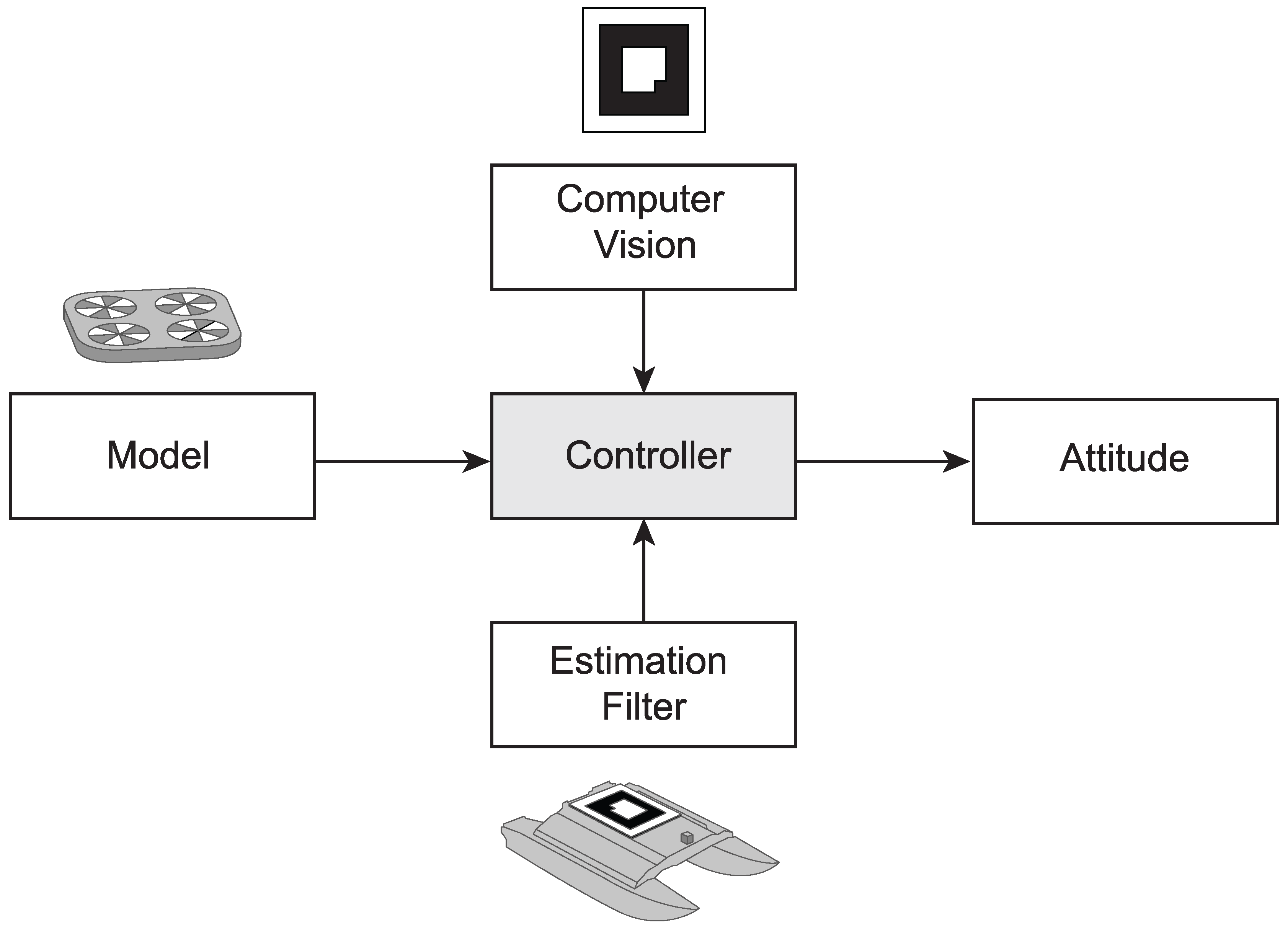
Figure 2.
Coordinate frames for the landing systems. represents the UAV’s pose with reference to the local frame and, in the same way, for the USV. and are the transformation between the down-looking camera and frontal cameras, respectively, and the vehicle’s body frame. and are the pose from the visual marker to the UAV and to the USV, respectively. Finally, is the pose from the USV to the UAV.
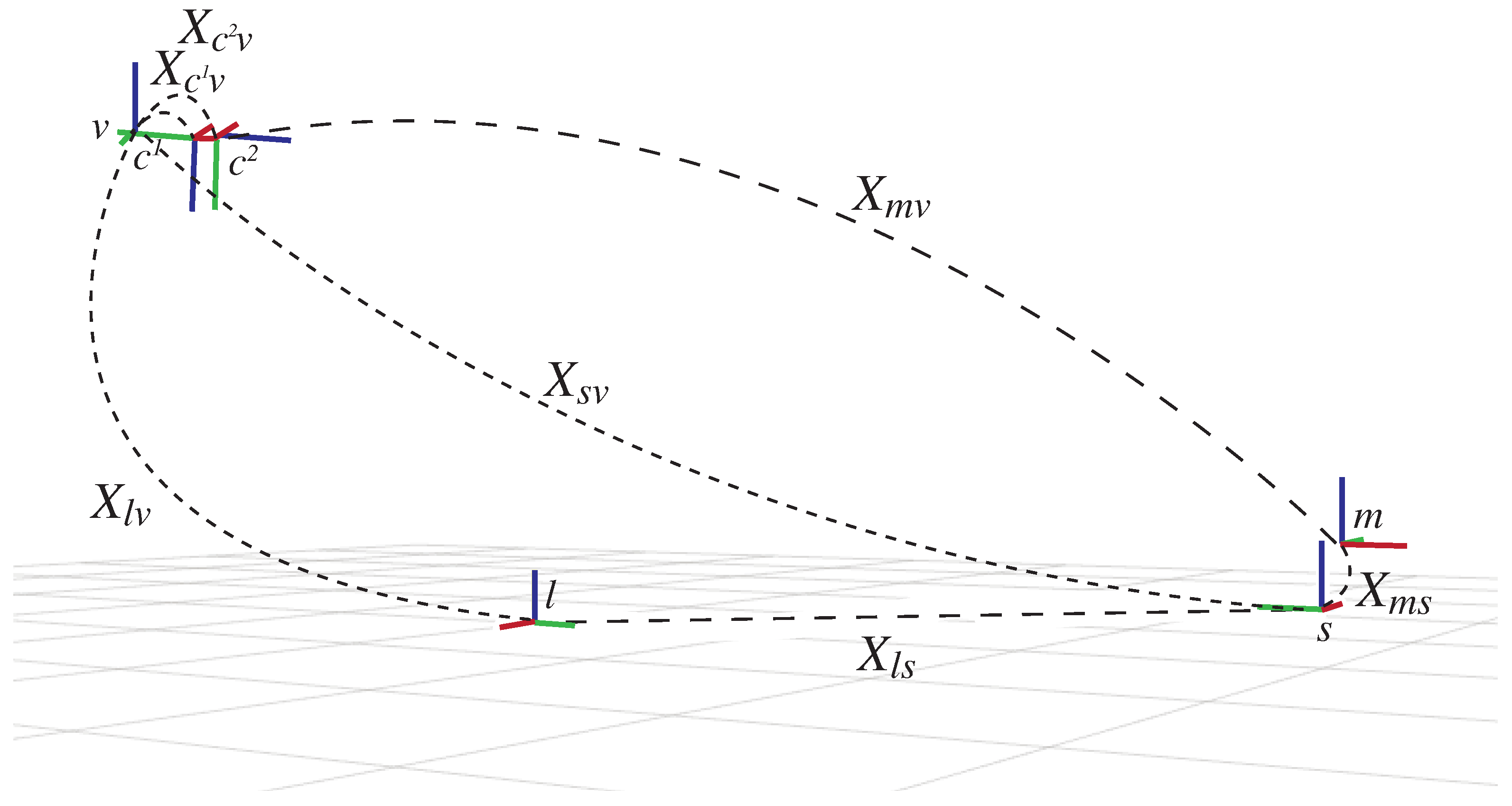
Figure 3.
The image processing algorithm estimates the distances between the UAV and the visual marker.
Figure 3.
The image processing algorithm estimates the distances between the UAV and the visual marker.
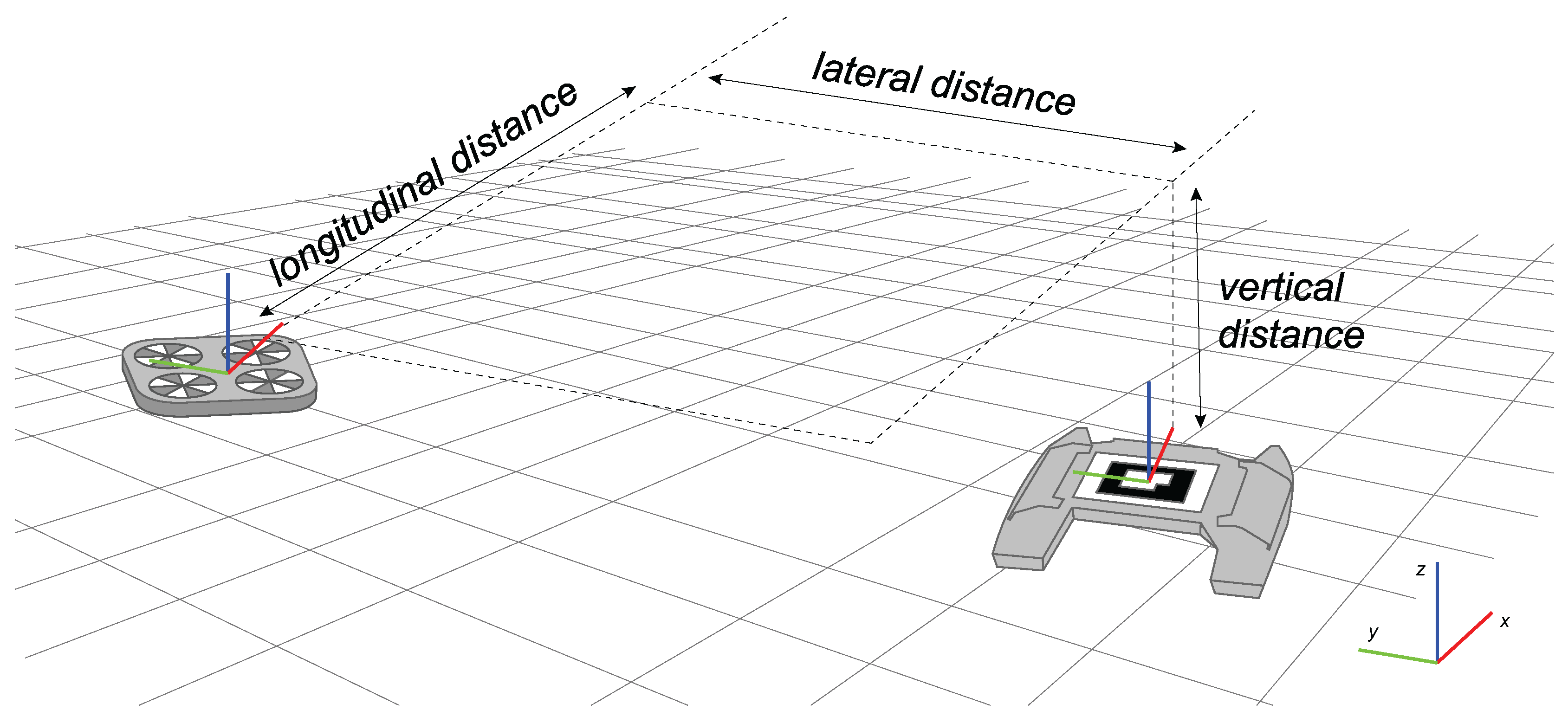
Figure 4.
The movements around the vertical, longitudinal and lateral axis of the USV are called yaw, roll and pitch, respectively.
Figure 4.
The movements around the vertical, longitudinal and lateral axis of the USV are called yaw, roll and pitch, respectively.

Figure 5.
Controller commands and visual offsets in the experiment with a rolling landing platform.

Figure 6.
(Top) The UAV and USV 3D trajectories, in blue and red, respectively, in the UAV’s reference frame. (Bottom) The roll disturbances to which the USV is subjected.
Figure 6.
(Top) The UAV and USV 3D trajectories, in blue and red, respectively, in the UAV’s reference frame. (Bottom) The roll disturbances to which the USV is subjected.
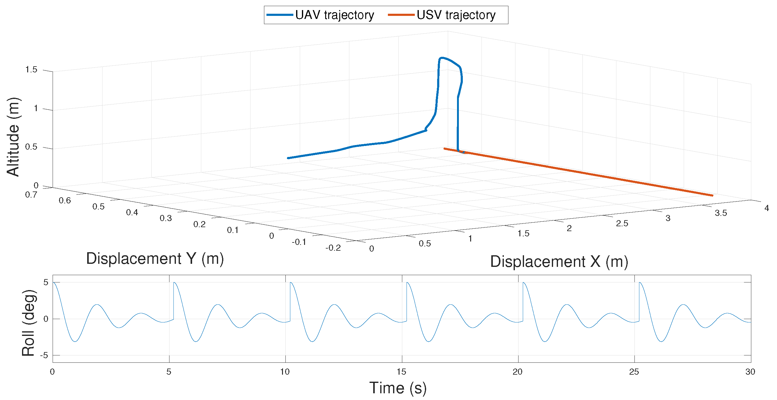
Figure 7.
Landing manoeuvre of a vertical take-off and landing (VTOL) UAV on a USV subject only to rolling disturbances. The drone approach the deck first using its frontal camera (a–b) until the marker is not visible anymore (c). At this point, the altitude of the UAV is increased (d) while the bottom downward-looking camera is used for the tracking of the marker (e) and accomplish the landing manoeuvre (f).
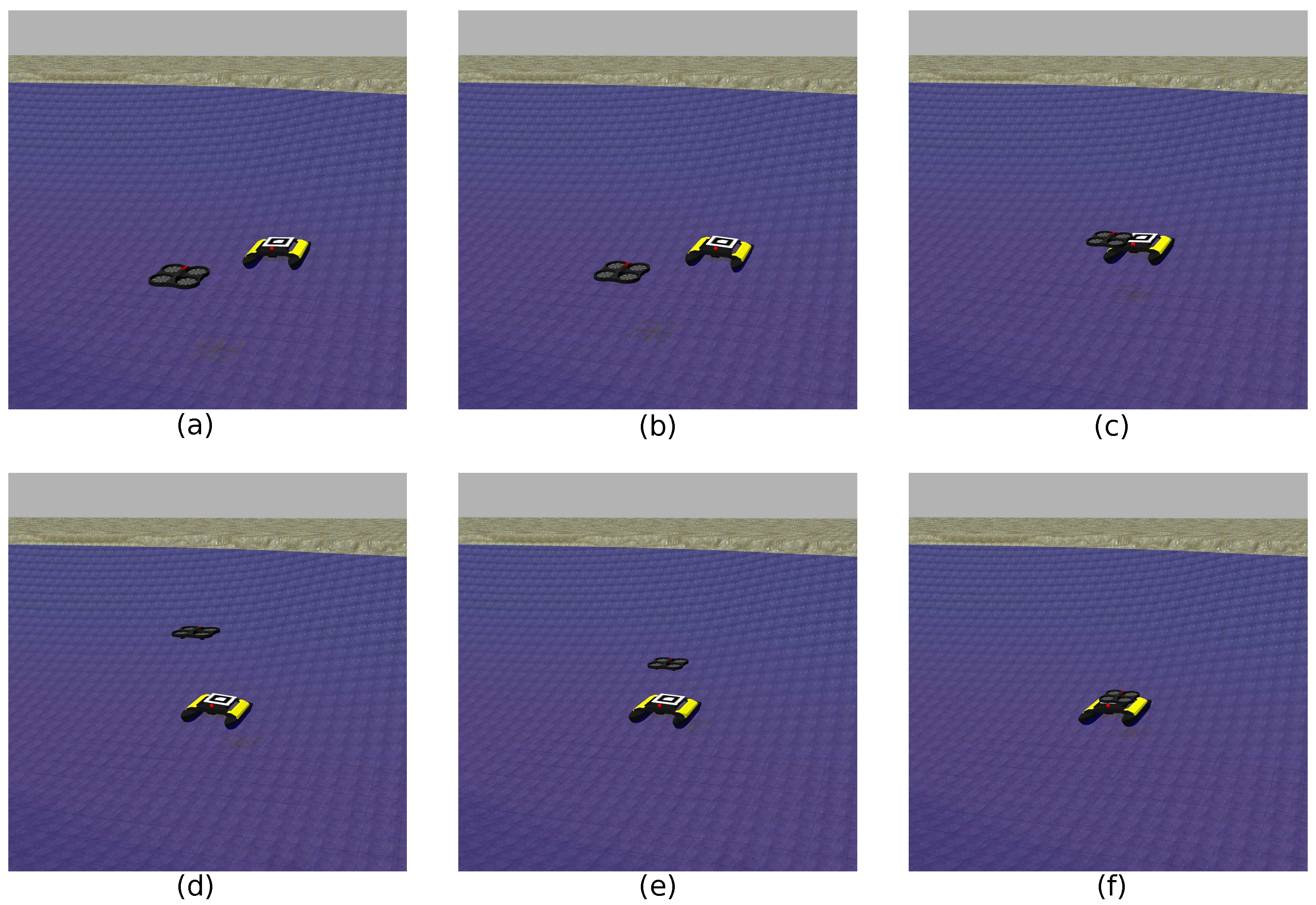
Figure 8.
(Top) The UAV and USV 3D trajectories, in blue and red, respectively, in the UAV’s reference frame. (Bottom) The pitch disturbances to which the USV is subjected.
Figure 8.
(Top) The UAV and USV 3D trajectories, in blue and red, respectively, in the UAV’s reference frame. (Bottom) The pitch disturbances to which the USV is subjected.

Figure 9.
Controller commands and visual offsets in the experiment with a pitching landing platform.
Figure 9.
Controller commands and visual offsets in the experiment with a pitching landing platform.
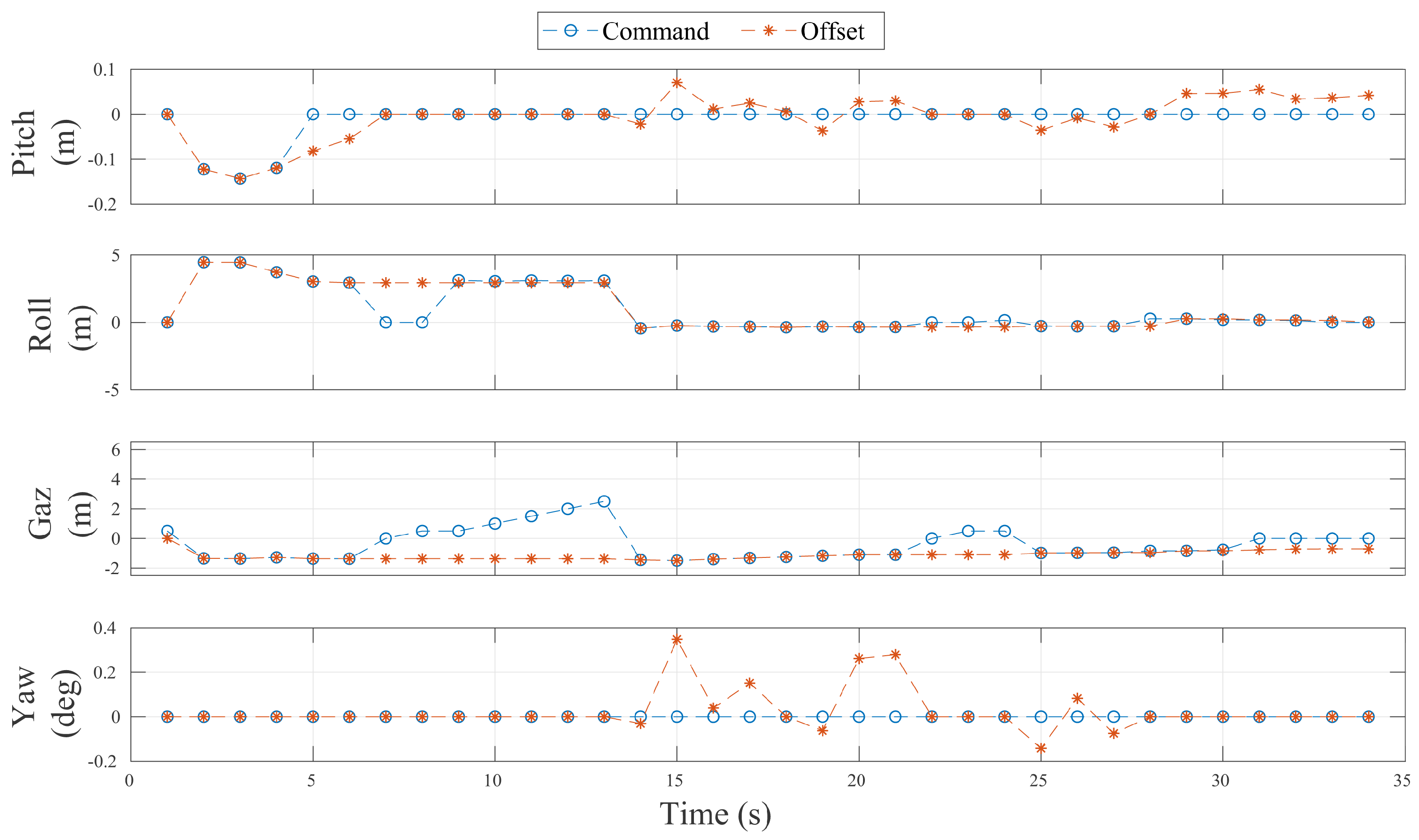
Figure 10.
Landing manoeuvre of a VTOL UAV on a USV subject only to pitching disturbances. The drone approach the deck first using its frontal camera (a–b) until the marker is not visible anymore (c). At this point, the altitude of the UAV is increased (d) while the bottom downward-looking camera is used for the tracking of the marker (e) and accomplish the landing manoeuvre (f).

Figure 11.
(Top) The UAV and USV 3D trajectories, in blue and red, respectively, in the UAV’s reference frame. (Bottom) Both the roll and pitch disturbances to which the USV is subjected.
Figure 11.
(Top) The UAV and USV 3D trajectories, in blue and red, respectively, in the UAV’s reference frame. (Bottom) Both the roll and pitch disturbances to which the USV is subjected.

Figure 12.
Controller commands and visual offsets in the experiment with a pitching and rolling landing platform, in order to simulate complex marine scenarios.
Figure 12.
Controller commands and visual offsets in the experiment with a pitching and rolling landing platform, in order to simulate complex marine scenarios.

Figure 13.
Landing manoeuvre of a VTOL UAV on a USV subject to both rolling and pitching disturbances, in order to simulate complex marine scenarios. The drone approach the deck first using its frontal camera (a–b) until the marker is not visible anymore (c). At this point, the altitude of the UAV is increased (d) while the bottom downward-looking camera is used for the tracking of the marker (e) and accomplish the landing manoeuvre (f).

Table 1.
The controller parameters used in the simulation performed.
| Parameter | Value | Parameter | Value |
|---|---|---|---|
| K_direct | 5.0 | K_rp | 0.3 |
| droneMass (kg) | 0.525 | max_yaw (rad/s) | 1.0 |
| xy_damping_factor st19 | 0.65 | max_gaz_rise (m/s) | 1.0 |
| max_gaz_drop (m/s) | −0.1 | max_rp | 1.0 |
© 2018 by the authors. Licensee MDPI, Basel, Switzerland. This article is an open access article distributed under the terms and conditions of the Creative Commons Attribution (CC BY) license (http://creativecommons.org/licenses/by/4.0/).
Share and Cite
MDPI and ACS Style
Polvara, R.; Sharma, S.; Wan, J.; Manning, A.; Sutton, R. Vision-Based Autonomous Landing of a Quadrotor on the Perturbed Deck of an Unmanned Surface Vehicle. Drones 2018, 2, 15. https://doi.org/10.3390/drones2020015
AMA Style
Polvara R, Sharma S, Wan J, Manning A, Sutton R. Vision-Based Autonomous Landing of a Quadrotor on the Perturbed Deck of an Unmanned Surface Vehicle. Drones. 2018; 2(2):15. https://doi.org/10.3390/drones2020015
Chicago/Turabian StylePolvara, Riccardo, Sanjay Sharma, Jian Wan, Andrew Manning, and Robert Sutton. 2018. "Vision-Based Autonomous Landing of a Quadrotor on the Perturbed Deck of an Unmanned Surface Vehicle" Drones 2, no. 2: 15. https://doi.org/10.3390/drones2020015