Use of UAV-Borne Spectrometer for Land Cover Classification

1
Geomatics Engineering, Department of Earth & Space Science & Engineering, Lassonde School of Engineering, York University, Toronto, ON M3J 1P3, Canada
2
Space Engineering, Department of Earth & Space Science & Engineering, Lassonde School of Engineering, York University, Toronto, ON M3J 1P3, Canada
*
Author to whom correspondence should be addressed.
Drones 2018, 2(2), 16; https://doi.org/10.3390/drones2020016
Submission received: 20 March 2018
/
Revised: 13 April 2018
/
Accepted: 17 April 2018
/
Published: 20 April 2018
(This article belongs to the Special Issue Latest Developments, Methodologies and Applications Based on UAV Platforms)
Abstract
:Unmanned aerial vehicles (UAV) are being used for low altitude remote sensing for thematic land classification using visible light and multi-spectral sensors. The objective of this work was to investigate the use of UAV equipped with a compact spectrometer for land cover classification. The UAV platform used was a DJI Flamewheel F550 hexacopter equipped with GPS and Inertial Measurement Unit (IMU) navigation sensors, and a Raspberry Pi processor and camera module. The spectrometer used was the FLAME-NIR, a near-infrared spectrometer for hyperspectral measurements. RGB images and spectrometer data were captured simultaneously. As spectrometer data do not provide continuous terrain coverage, the locations of their ground elliptical footprints were determined from the bundle adjustment solution of the captured images. For each of the spectrometer ground ellipses, the land cover signature at the footprint location was determined to enable the characterization, identification, and classification of land cover elements. To attain a continuous land cover classification map, spatial interpolation was carried out from the irregularly distributed labeled spectrometer points. The accuracy of the classification was assessed using spatial intersection with the object-based image classification performed using the RGB images. Results show that in homogeneous land cover, like water, the accuracy of classification is 78% and in mixed classes, like grass, trees and manmade features, the average accuracy is 50%, thus, indicating the contribution of hyperspectral measurements of low altitude UAV-borne spectrometers to improve land cover classification.
1. Introduction and Objectives
In recent times, small UAV platforms have been extensively used for low altitude remote sensing and thematic land cover classification, which is one of the main purposes of remote sensing. Usually, light weight multispectral, hyperspectral and thermal imaging sensors are used. Recently, a growing number of studies have been focusing on UAV-borne spectrometers, which are now becoming lighter and more compact [1,2,3,4]. A spectrometer measures the spectral signatures of all ground features within the sensor's field of view by analyzing the spectral characteristics of light radiation and breaking down the incoming energy into different wavelengths. Because of the light weight and reliable performance of the spectrometers, they are mounted on a UAV and used to capture data in several bands. While the optical, multispectral and hyperspectral cameras capture several bands of the electromagnetic spectrum and provide continuous gridded pixel area coverage, the spectrometer’s coverage consists of single pixel footprints determined by its field of view; however, its high spectral resolution makes it a good alternative to multispectral sensors. In this work, we present a land cover classification method using a UAV-borne spectrometer and a Raspberry pi camera mounted on the UAV. The UAV RGB images provide the exterior orientation of the camera sensor and orthoimagery, which are used to determine the position of the spectrometer and its ground footprint.
Currently, a growing number of studies have focused on object-based image classification techniques for land-cover mapping using high resolution UAV imagery [5,6,7,8]. Object-based classification produced higher accuracy than pixel-based classification [9]. Hence in this study, object-based image classification has been used to validate the classification produced using spectrometer data.
2. Related Studies
An automated classification has been performed using a UAV combining hyper-spectral radiometers and multi-spectral cameras to develop thematic maps based on the interaction of VIS-NIR spectrometers with MSI cameras [8]. The data were analyzed using a modified unsupervised approach based on a fast k-means algorithm. The resulting classification was used to derive thematic object maps using a hybrid approach which combined the advantages of pixel and object-based algorithms.
The performance of new light-weight multispectral sensors for micro-UAV and their application have been studied in agronomical research and precision farming applications [10,11]. Lightweight multispectral and thermal imaging sensors have also been used for remote sensing vegetation from UAV platforms [12]. Thermal imager and hyperspectral sensor in visible-NIR bands have been used on fixed wing and quadcopter platforms [13,14]. UAS hyperspectral imagery has been used for leaf area index estimation [15,16] while UAS thermal images have been used to monitor stream temperatures [17] and roof heat losses [18].
A UAV-borne spectrometer was synchronized with a ground one to investigate the fast airborne acquisition of hyperspectral measurements over large areas as a useful complement for conventional field spectroscopy [1]. A UAV spectrometer system carried on an octocopter UAV has been developed as part of a multi-sensor approach for multi-temporal assessment of crop parameters [19]. A lightweight unmanned aerial vehicle (UAV)-based spectrometer system was employed to measure water reflectance measured and assess environmental impacts [3]. The spectrometer has also been used to compute the NDVI for agronomic applications [20] while a new method was developed to measure reflectance factor anisotropy using a pushbroom spectrometer mounted on a multicopter UAV [21]. A lightweight hyperspectral mapping system (HYMSY) has been developed for rotor-based UAV to study the prospects for agricultural mapping and monitoring applications [2]. The HYMSY was an integration of a custom-made pushbroom spectrometer with a photogrammetric camera which is synchronized to a miniature GPS-Inertial Navigation System. The performance of a new Fabry–Perot interferometer-based (FPI) spectral camera has been investigated to collect spectrometric image blocks with stereoscopic overlaps using light-weight UAV platforms [4]. The processing and use of this new type of image data were explored to incorporate in precision agriculture.
However, we see that there are not much extensive studies on using UAV-borne spectrometers along with optical camera for land use classification. While there are some studies on multispectral and hyperspectral imaging spectrometers, there are no wide-ranging investigations on the use of single point spectrometers in remote sensing. Also, most of the studies have focused on the application of spectroscopy only in the visible range and not NIR spectroscopy [1,2,3]. To address these issues, in this study, we present an approach to obtain land cover classification using a FLAME-NIR spectrometer which has a preconfigured range from 950 to 1650 nm and a Raspberry pi camera mounted on the UAV.
3. System Description
3.1. The Platform
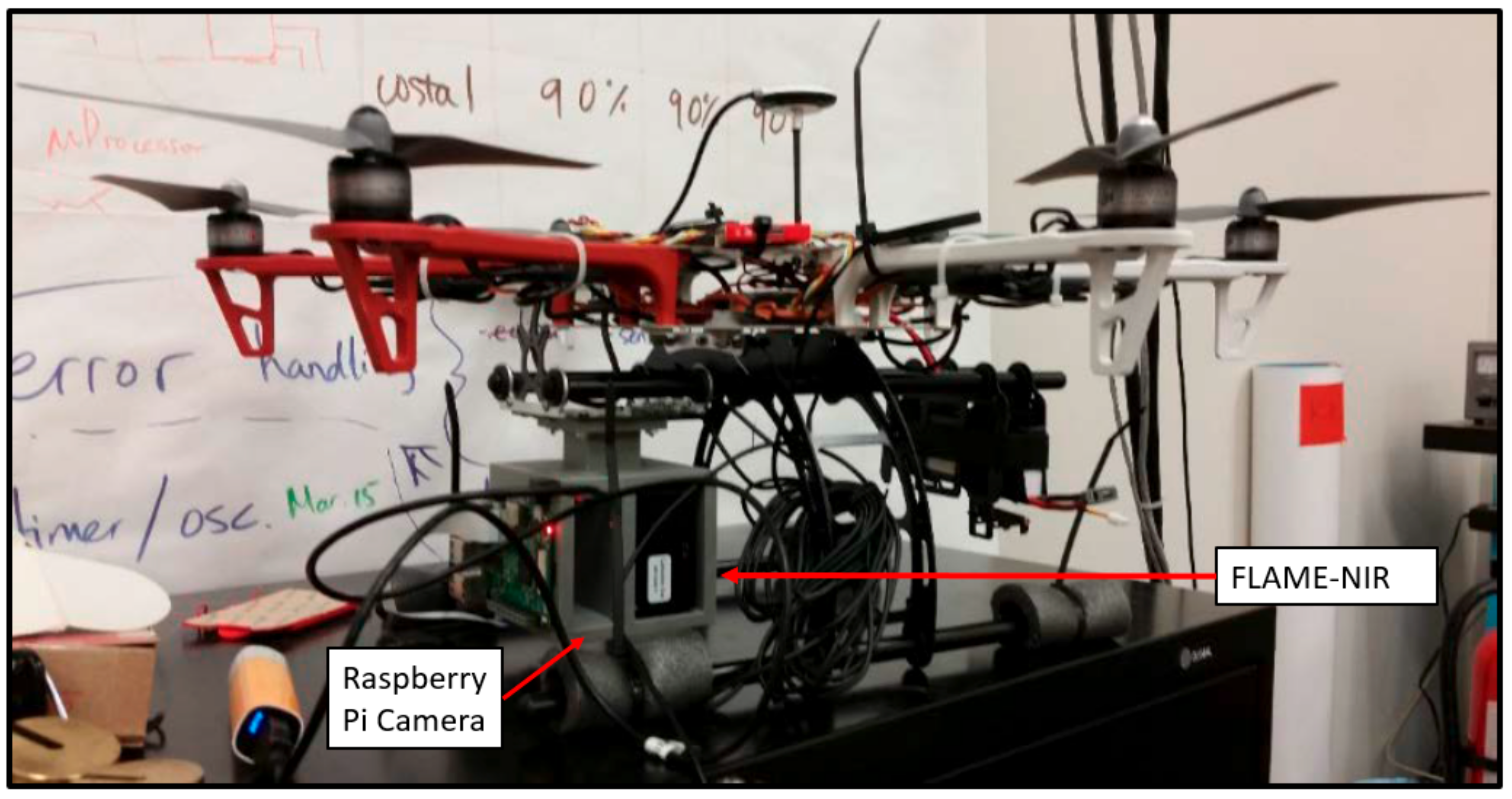
The UAV platform was the DJI Flamewheel F550 which was a battery powered vertical take-off and landing (VTOL) UAV with six coaxial motors with a total mass of 2.3 kg, including the payloads and landing gear. The sensor payloads were a FLAME-NIR spectrometer manufactured by Ocean Optics and a Raspberry Pi camera pointing in the nadir direction. The spectrometer and camera module were integrated into a single mount and linked together to a Raspberry Pi 3 computer, which served to run each system and store the data for post-processing, as shown in Figure 1. The spectrometer and the camera were mounted on the forward side of the UAV and below the arms on the landing gear. The battery for the UAV flight was mounted on the gear and on the opposite side of the payload making the system balanced. Prior to the flight, the UAV was properly balanced by sliding the battery mount along the rails of the landing gear.
The FLAME-NIR spectrometer was fitted with an Ocean Optics 74-DA collimating lens at the entrance slit for capturing the incident light. It weighs 265 g and acquires hyperspectral measurements by operating in the 927 nm to 1658 nm near infrared (NIR) spectral region, with spectral resolution less than 10 nm. The collimating lens has a focal length of 5 mm and a diameter of 10 mm, corresponding to a field of view of 5° × 2.5° due to the slit size of 1 mm × 25 μm. The Raspberry Pi camera module version 2.1 included a sensor with a rectangular 62.2° × 48.8° field of view and a focal length of 3.04 mm which was used to capture optical imagery.
3.2. Spectrometer Radiometric Calibration
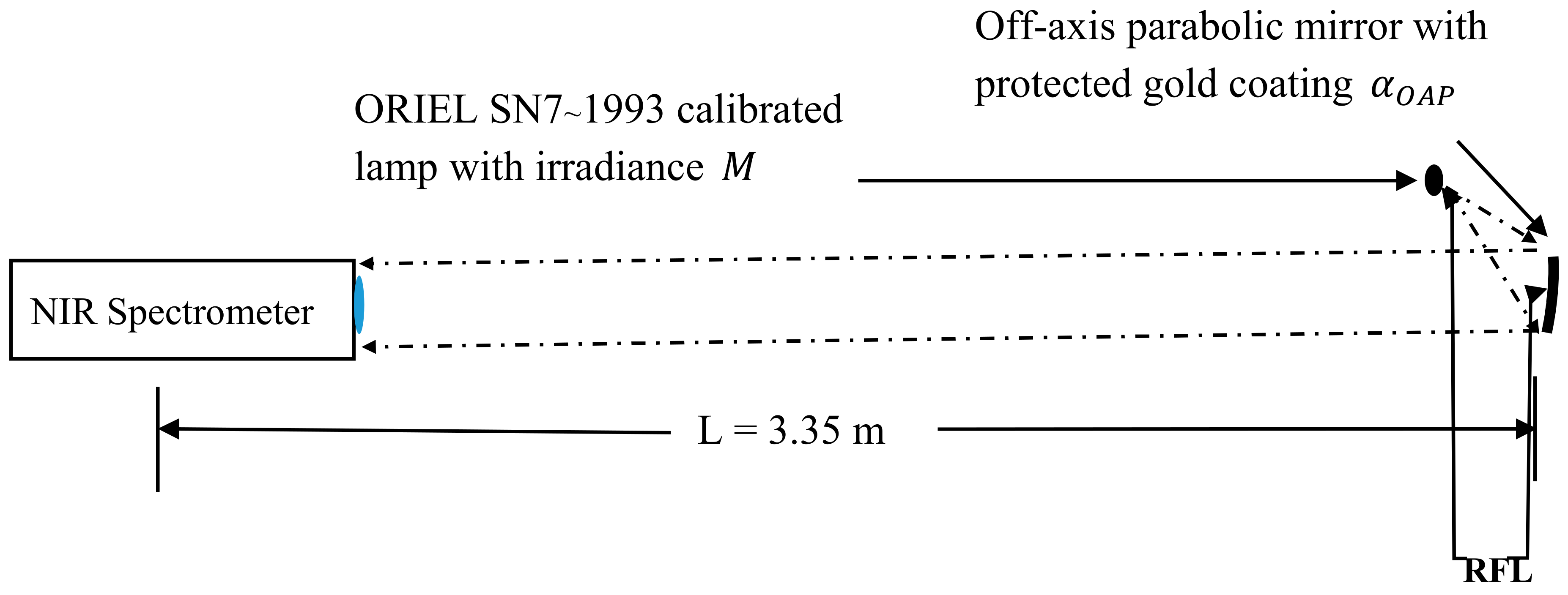
The radiometric calibration of FLAME-NIR spectrometers involves relating the energy received by the instrument to the number of detector counts measured by the detector electronics of the instrument. It is performed using the SpectraSuite spectrometer operating software [22] with the help of a calibrated light source (DH 2000-CAL), and an off-axis parabolic mirror (OAP) as shown in Figure 2.
The light is collimated from the lamp using OAP in the direction of the spectrometer. The spectrometer mounted on a rotation stage is placed in the line of the collimated light. The rotation stage is used to rotate the spectrometer so that its optics are perpendicular to the collimated light. Initially, the instrument settings, such as exposure time, are set to high values in order to saturate the instrument to easily detect the instrument reaching the correct orientation as it is rotated. The data from the spectrometer is monitored as it is rotated using the rotation stage to ensure that all the pixels of the detector reach maximum saturation. At the point that all the pixels reach maximum saturation, the instrument is properly aligned relative to the collimated light and the calibration can be performed. While the calibration process is being performed, a non-reflective black foil is used to surround the lamp and mirror in order to reduce the effect of the stray on the calibration. The use of a calibrated lamp and off-axis parabolic mirror for collimation is a common technique for the calibration of infrared detectors, as described in [23].
Once the spectrometer was in the correct orientation, data was collected using the spectrometer at a series of instrument settings at which two criteria were met:
- -
- the instrument was not saturated at all pixels.
- -
- the number of counts on the detector was distinguishable from background noise signal at all pixels.
The calibration equations used are based on the assumption that the irradiance M of the ORIEL SN7~1993 calibrated lamp can be treated as a point source. The irradiance of the lamp is provided by Newport at a distance 1 = 50 cm, which is then adjusted using the inverse square law to the reflected focal length RFL of the OAP mirror, as this is the distance between the lamp and the center of the mirror in the experimental setup. Further scaling of the irradiance is then performed to take into account the reflectance α_OAP of the OAP mirror, which is a function of wavelength, and the angle θ between the OAP mirror and the spectrometer field of view (FOV). The irradiance is then converted to energy by multiplying it by the exposure time setting of the instrument.
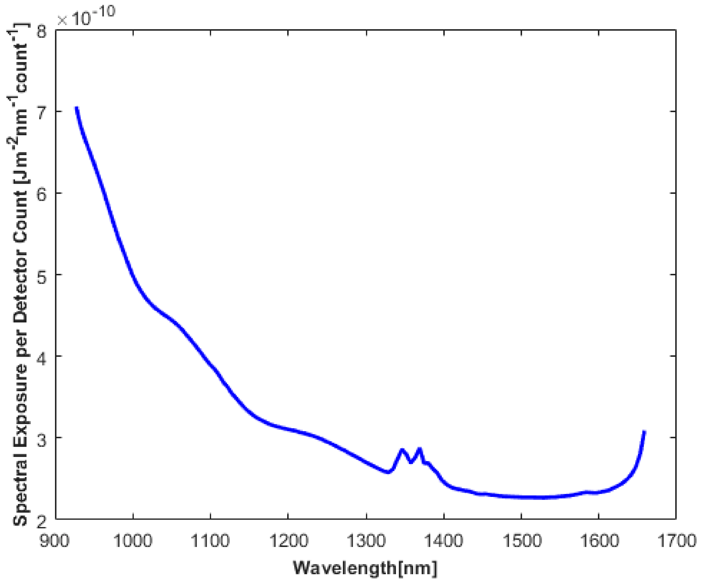
Radiometric calibration was performed by dropping the power from the lamp to 250 W, 500 W, and 750 W so that adequate quantities of data at different exposure time settings could be obtained. The irradiance of the lamp was assumed to scale linearly with reduced power, i.e., the irradiance curve of the lamp was scaled by the ratio of output power over 1000 W. For each data set, 1000 spectral measurements were made with the FLAME-NIR, resulting in a total of eight data sets. Six data sets were acquired at varying exposure times but with a lamp output power of 250 W, while the remaining data sets were acquired with a lamp output power of 500 W and 750 W, respectively. This proportion of data sets were selected because at 500 W and 750 W, there was a high level of saturation at any exposure time setting greater than 1 ms. A spectral exposure per detector count conversion function was computed for the FLAME-NIR and is shown in Figure 3.
The conversion function shown in Figure 3 is the mean of all the conversion functions computed for each measurement of each data set. The curve deviation from the theoretical blackbody curve, peaks within 1300 nm and 1400 nm, is attributed to errors caused by the diffraction grating, spectrometer lens, off-axis parabolic mirror, and detector quantum efficiency.
4. Study Area and Data Collection
The field campaign was conducted near Chaffey’s lock, Ontario, Canada, on 5 November 2016. The test area was about 200 m × 100 m. UAV RGB images and spectrometer data were collected through five flights under clear sky conditions with FLAME-NIR spectral measurements and optical RGB images acquired at regular intervals one spectrometer measurement being made followed by a corresponding camera image being taken. Spectral measurements were acquired at an exposure time setting of 750 ms based on ground experiments conducted prior to the actual flight on different surfaces to avoid saturation and be able to detect reflection changes and provide a clear difference signal between measurements made over different land cover features such as land and water.
The flying height was about 40 m above ground. The flight altitude was selected mainly based on having better visual contact for operating the UAV and be below the allowable ceiling of 90 m. It also allowed for a larger number of images and denser spectrometer footprint coverage. This also resulted in a denser digital surface model from a dense image matching process. At the start of acquisition of each data set, the UAV needed to acquire GPS satellite signals before it would begin its flight. A white panel was used to test suitable spectrometer exposure time settings prior to the airborne campaign. This process involved setting the white panel on the ground and moving the spectrometer over it multiple times at differing exposure time settings in order to determine which settings provided strong signals without saturating the instrument detector.
5. Methodology
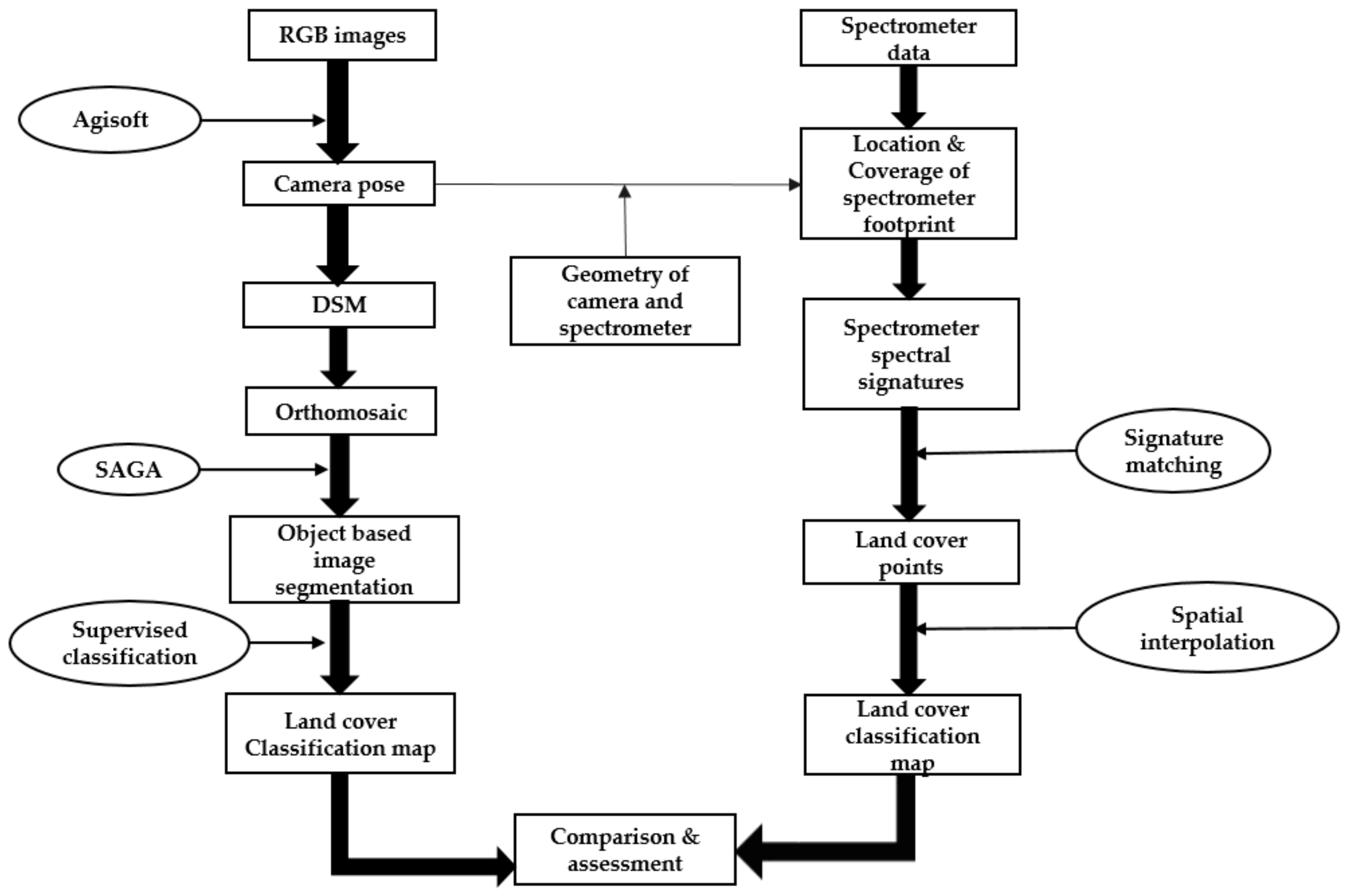
The collected data were processed and utilized for land cover classification following a workflow as shown in Figure 4. Each process is explained in detail in the following sections.
5.1. Camera Pose Estimation
Agisoft PhotoScan [24] was used to process the RGB images. The total number of images were 294 with resolution 2592 × 1944 pixels. Camera calibration was incorporated into the adjustment solution. The exterior orientation parameters of 268 images were estimated using bundle adjustment based on a local reference system defined by the ground control points. The control points RMSE were 3.5, 2.2 and 3.5 cm, respectively, in X, Y, and Z. One check point was used with error 3.5 cm in X, 2.2 cm in Y and 3.5 cm in Z, respectively. A very dense Digital Surface Model (DSM) was generated with 853 points/m2 and the final orthoimage mosaic was generated at 2 cm spatial resolution. The camera locations plotted on the orthoimage mosaic are shown in Figure 5.
5.2. Spectrometer Positioning and Footprint Determination
The spatial geometry of the camera and spectrometer in the mounting system was used to estimate the ground location of the spectrometer field of view (FOV) with respect to the camera ground FOV. The relative geometry of the Raspberry Pi camera module analogous to that of the FLAME-NIR spectrometer and their corresponding rectangular and elliptical fields of view are shown in Figure 6. The center of the field of view of the FLAME-NIR is offset from the center of the camera image by offsets ΔX, ΔY, and ΔZ, which are measured values from the design of the mounting system. Angles θX and θY are the Raspberry Pi camera field of view angles of 62.2° and 48.8° respectively, while α and β are the spectrometer field of view angles of 2.5° and 5° respectively due to the 74-DA lens. The areas on the ground covered by the lenses of the camera, (2LX by 2LY), and of the spectrometer, (major and minor axes 2LA and 2LC of the ellipse), were calculated using the flying height H of the camera above the ground and the angular fields of view of the two sensors.
The location and size of the spectrometer footprint were determined using the linear offsets between the camera module and spectrometer, exterior orientation parameters of the RGB images, and the optical geometry of the spectrometer. The orientation of the major axis of the spectrometer’s footprint ellipse was estimated using the kappa orientation angle of the image. Since the flying height above ground is low and the magnitude of the omega and phi angles was quite small, their effect was not taken into account. Similarly, the DSM was not used as the topographic relief of the area was very small and, therefore, flat terrain surface was assumed.
The lengths LA and LC of the ground elliptical footprint of the spectrometer corresponding to the semi-major and semi-minor axes in the along-flight and cross-flight directions, respectively are given by:
At 40 m flying height, the lengths of the major and minor axes were about 3.50 m and 1.75 m, respectively. The locations of the spectrometer footprints are shown in Figure 7.
5.3. Spectrometer Spectral Signatures
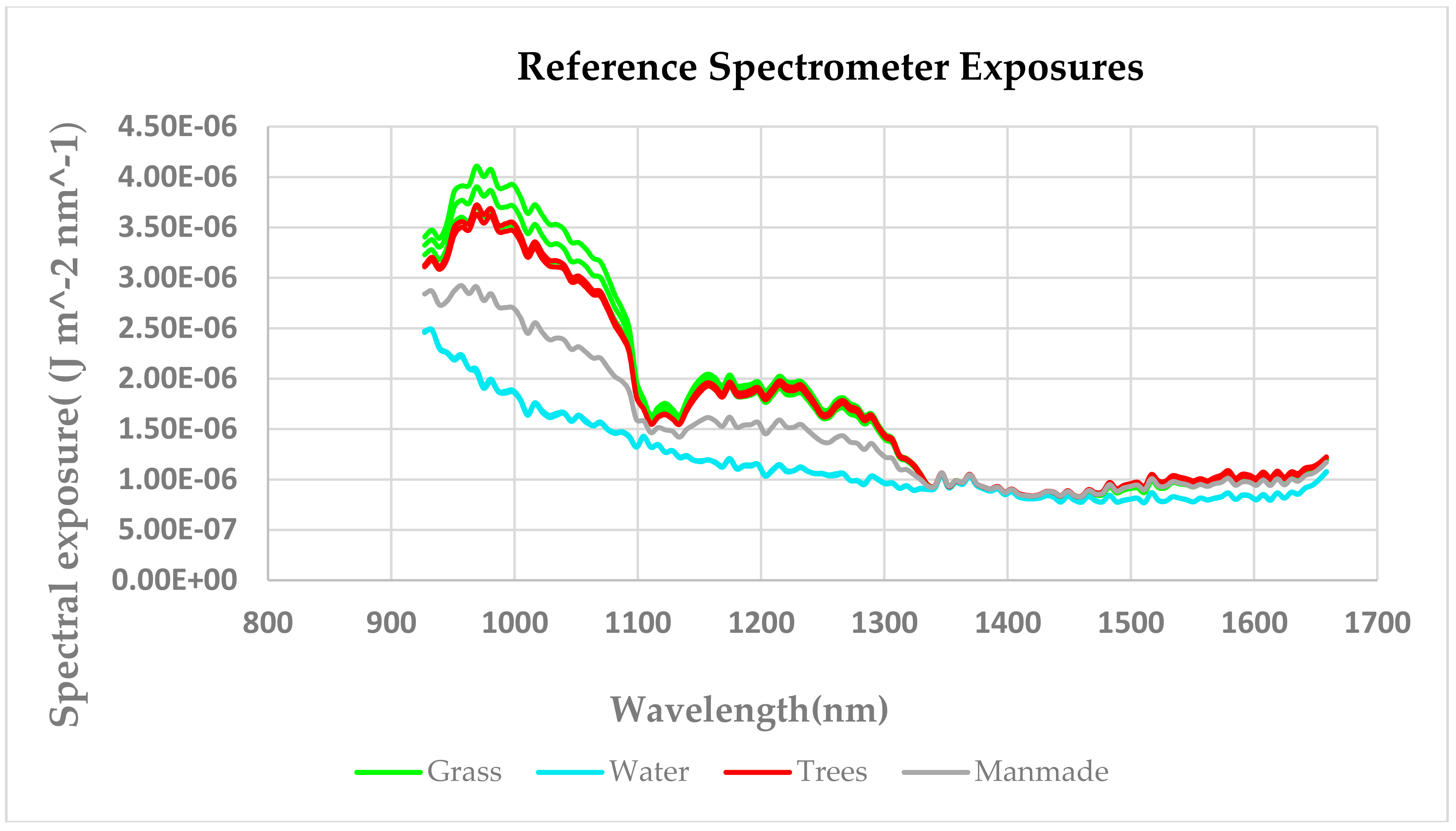
For each of the spectrometer ground ellipses, the spectral exposure is calculated by multiplying the detector counts with the conversion function computed from the spectrometer calibration. The calculated spectral exposure was plotted against wavelength indicating the land cover signature at the footprint location which is shown in Figure 8. The labeling of the plot was based on a-priori information and visual inspection of the corresponding RGB image. Based on these signature plots, various land cover elements such as grass, water, tree and manmade features could be distinguished. Trees and grass exhibit similar behavior throughout the NIR region with a drastic fall in detector counts around 1100 nm and 1340 nm due to water content. During analysis, the values were capped at 1340 nm wavelength since all land cover classes exhibited similar responses beyond it.
5.4. Signature Matching and Assessment
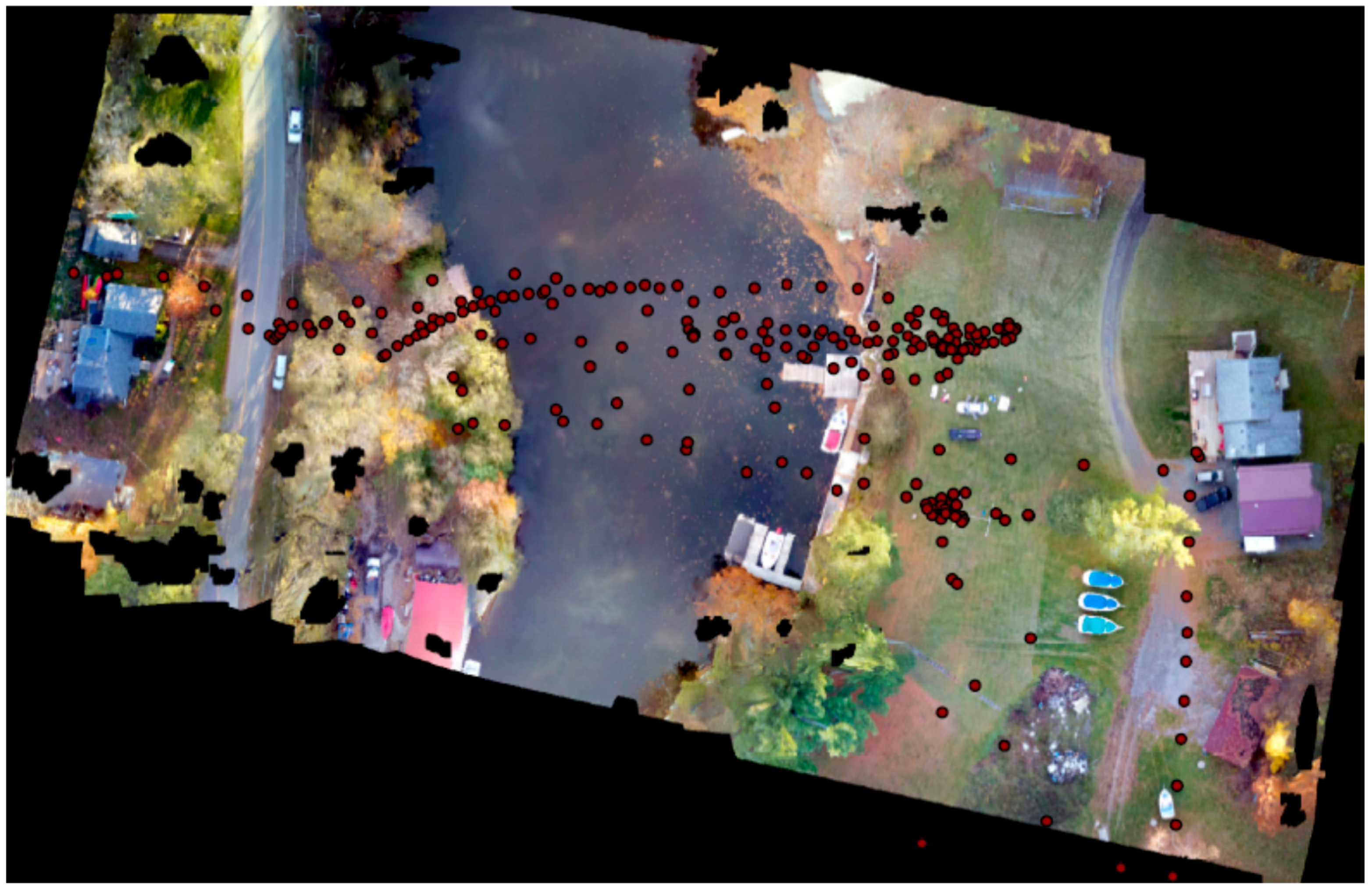
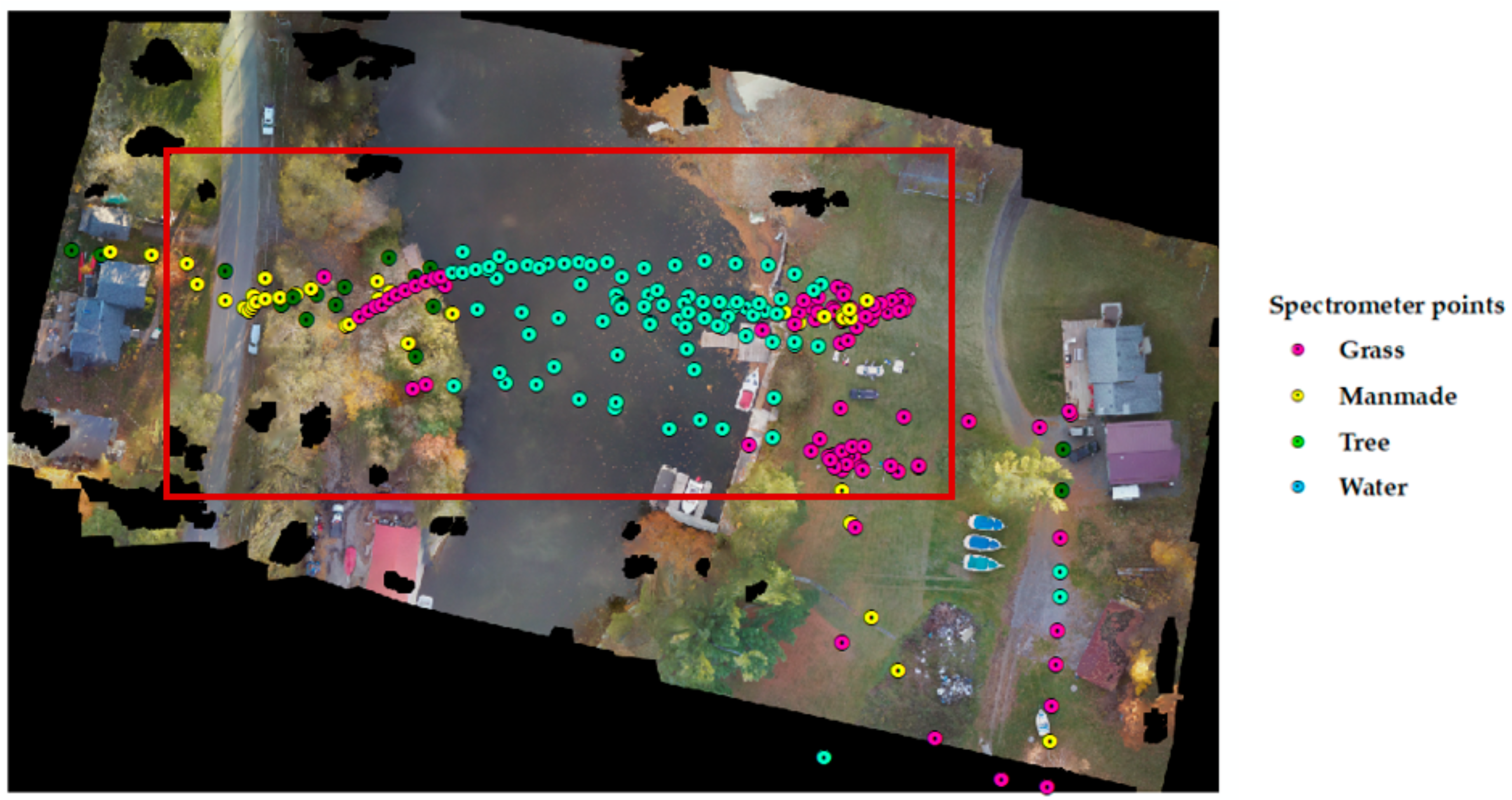
For the purpose of training, three to five sample spectrometer ellipses were identified for each land cover class which had homogeneous footprint coverage. Spectral exposure was calculated and the average values were used as training samples. Then, the spectral exposure of all ellipse footprints was matched to the training samples by means of Root Mean Square Error (RMSE) and their centers were labeled, thus, generating a set of irregular land cover points. The spectrometer points are overlaid on the RGB orthomosaic as shown in Figure 9. The accuracy of the matching was assessed based on confusion matrix which is shown in Table 1. Overall accuracy, false positives, and negatives were obtained from the confusion matrix. The overall accuracy was estimated to be 81.18%.
5.5. Land Cover Classification and Assessment
As spectrometer data do not provide continuous terrain coverage; spatial interpolation was carried out using the inverse distance weighted technique from the irregularly distributed labeled spectrometer points, thus, generating a continuous land cover classification map of 20 cm resolution, as shown in Figure 10. Before interpolation, a visual assessment was done to remove the outliers. During processing, the extent of interpolation was limited to the region where the spectrometer points were concentrated as shown by the red bounding box in Figure 9.
Object Based Land Cover Classification Using RGB Images
The RGB images acquired during the flight were used to generate an object-based land cover classification map to validate the classification map produced by the interpolation of labeled spectrometer points. The classification was executed in two stages, imagery segmentation and object classification. The imagery segmentation of the RGB orthomosaic was performed with SAGA [25]. This software implements image segmentation using a seeded region growing algorithm. It was then followed by object classification using a maximum likelihood classifier for which the training areas were chosen based on a-priori knowledge. The resulting classification map is shown in Figure 11.
6. Results and Discussion
The generated object-based image segmentation was used as reference land cover to assess the accuracy of the classification map produced by the interpolation of labeled spectrometer points. For this purpose, spatial overlay operation was carried out between the two classification map layers to compute the spatially intersected (common) land cover regions between them. The land cover classes on the spectrometer classification intersecting with different classes on object-based classification are shown in Figure 12 and the cross-tabulated area of the intersecting classes is shown in Table 2.
The percentage of the areas of grass, water, trees and manmade classes overlapped in both classification methods was 58%, 78%, 48% and 45%, respectively. We see that 12% of the area in grass, 20% in water, 27% in trees and 32% in manmade features are misclassified. The percentage of the overlapped area of water was reasonable as the result of the homogeneity in the class whereas the land in the study area was quite heterogeneous with diverse trees and manmade features which could not be captured well by the spectrometer footprints. The roads being a linear feature and since the spectrometer data collected over the roads were few, the interpolation of spectrometer points was not effective in classifying the roads.
7. Concluding Remarks
This work presents the use of a lightweight compact UAV spectrometer for land cover classification. Photogrammetric bundle adjustment solution from the RGB images was used to define the size and location of the spectrometer footprints. For each of the spectrometer ground ellipses, the land cover signature at the footprint location was determined based on which different land cover elements were distinguished. Spatial interpolation was executed on the land cover spectrometer points to obtain a thematic land cover classification map. The accuracy of the classification map was assessed using spatial intersection with the object-based classification performed using RGB images. Based on the preliminary results, it is observed that in homogeneous land cover, such as water, the classification accuracy is 78% while in mixed land cover, such as grass, trees and manmade features, the average accuracy is 50% showing that hyperspectral data from low altitude UAV-borne spectrometers can be used effectively to achieve thematic land cover classification. Further investigation can be carried out on using different graph matching techniques for signature matching for spectrometer footprints. Since object-based image classification has some unknown classes in itself, some ground truth points could be collected to better evaluate the accuracy of classification using spectrometer points. Also, it is suggested to collect more spectrometer data, especially on heterogeneous land cover areas so that the elliptical footprints are denser which can improve spatial interpolation.
Acknowledgments
This work is financially supported by the Natural Sciences and Engineering Research Council of Canada (NSERC) and York University.
Author Contributions
S.N. and C.A. conceived and designed the experiments; C.A., G.B., and R.L., collected data; S.N. and G.B performed the experiments; S.N. analyzed the data; S.N. drafted the paper. S.N and C.A contributed to its final version.
Conflicts of Interest
The authors declare no conflict of interest.
References
- Burkart, A.; Cogliati, S.; Schickling, A.; Rascher, U. A novel UAV-based ultra-light weight spectrometer for field spectroscopy. IEEE Sens. J. 2014, 14, 62–67. [Google Scholar] [CrossRef]
- Suomalainen, J.; Anders, N.; Iqbal, S.; Roerink, G.; Franke, J.; Wenting, P.; Hünniger, D.; Bartholomeus, H.; Becker, R.; Kooistra, L. A lightweight hyperspectral mapping system and photogrammetric processing chain for unmanned aerial vehicles. Remote Sens. 2014, 6, 11013–11030. [Google Scholar] [CrossRef]
- Zeng, C.; Richardson, M.; King, D.J. The impacts of environmental variables on water reflectance measured using a lightweight unmanned aerial vehicle (UAV)-based spectrometer system. ISPRS J. Photogramm. Remote Sens. 2017, 130, 217–230. [Google Scholar] [CrossRef]
- Honkavaara, E.; Saari, H.; Kaivosoja, J.; Pölönen, I.; Hakala, T.; Litkey, P.; Mäkynen, J.; Pesonen, L. Processing and assessment of spectrometric, stereoscopic imagery collected using a lightweight UAV spectral camera for precision agriculture. Remote Sens. 2013, 5, 5006–5039. [Google Scholar] [CrossRef] [Green Version]
- Akar, Ö. The Rotation Forest algorithm and object-based classification method for land use mapping through UAV images. Geocarto Int. 2016. [Google Scholar] [CrossRef]
- Lechner, A.M.; Fletcher, A.; Johansen, K.; Erskine, P. Characterising upland swamps using object-based classification methods and hyper-spatial resolution imagery derived from an Unmanned Aerial Vehicle. ISPRS Ann. Photogramm. Remote Sens. Spat. Inf. Sci. 2012, 1–4, 101–106. [Google Scholar] [CrossRef]
- Li, M.; Ma, L.; Blaschke, T.; Cheng, L.; Tiede, D. A systematic comparison of different object-based classification techniques using high spatial resolution imagery in agricultural environments. Int. J. Appl. Earth Obs. Geoinf. 2016, 49, 87–98. [Google Scholar] [CrossRef]
- Mancini, A.; Frontoni, E.; Zingaretti, P. A multi/hyper-spectral imaging system for land use/land cover using unmanned aerial systems. In Proceedings of the 2016 International Conference on Unmanned Aircraft Systems (ICUAS), Washington, DC, USA, 7–10 June 2016; pp. 1148–1155. [Google Scholar]
- Pande-Chhetri, R.; Abd-Elrahman, A.; Liu, T.; Morton, J.; Wilhelm, V.L. Object-based classification of wetland vegetation using very high-resolution unmanned air system imagery. Eur. J. Remote Sens. 2017, 50, 564–576. [Google Scholar] [CrossRef]
- Nebiker, S.; Lack, N.; Abächerli, M.; Läderach, S. Light-weight multispectral UAV sensors and their capabilities for predicting grain yield and detecting plant diseases. Int. Arch. Photogramm. Remote Sens. Spat. Inf. Sci. 2016, 41, 963–970. [Google Scholar] [CrossRef]
- Sona, G.; Passoni, D.; Pinto, L.; Pagliari, D.; Masseroni, D.; Ortuani, B.; Facchi, A. UAV multispectral survey to map soil and crop for precision farming applications. Int. Arch. Photogramm. Remote Sens. Spat. Inf. Sci. 2016, 41, 1023–1029. [Google Scholar] [CrossRef]
- Berni, J.A.J.; Zarco-Tejada, P.J.; Suárez, L.; González-Dugo, V.; Fereres, E. Remote Sensing of Vegetation from UAV Platforms Using Lightweight Multispectral and Thermal Imaging Sensors. Int Arch Photogramm Remote Sens Spat. Inf. Sci. 2009, Volume XXXVIII-1-4-7/W5. Available online: https://www.ipi.uni-hannover.de/fileadmin/institut/pdf/isprs-Hannover2009/Jimenez_Berni-155.pdf (accessed on 20 April 2018).
- Buettner, A.; Roeser, H.P. Hyperspectral Remote Sensing with the UAS “Stuttgarter Adler”—Challenges, Experiences and First Results. Int. Arch. Photogramm. Remote Sens. Spat. Inf. Sci. 2013, 1, 61–65. [Google Scholar] [CrossRef]
- Chrétien, L.P.; Théau, J.; Ménard, P. Wildlife multispecies remote sensing using visible and thermal infrared imagery acquired from an unmanned aerial vehicle (UAV). Int. Arch. Photogramm. Remote Sens. Spat. Inf. Sci. 2015, 40, 241–248. [Google Scholar] [CrossRef]
- Kalisperakis, I.; Stentoumis, C.; Grammatikopoulos, L.; Karantzalos, K. Leaf area index estimation in vineyards from UAV hyperspectral data, 2D image mosaics and 3D canopy surface models. Int. Arch. Photogramm. Remote Sens. Spat. Inf. Sci. 2015, 40, 299–303. [Google Scholar] [CrossRef]
- Proctor, C.; He, Y. Workflow for building a hyperspectral UAV: Challenges and opportunities. Int. Arch. Photogramm. Remote Sens. Spat. Inf. Sci. 2015, 40, 415–419. [Google Scholar] [CrossRef]
- Jensen, A.M.; Neilson, B.T.; McKee, M.; Chen, Y. Thermal remote sensing with an autonomous unmanned aerial remote sensing platform for surface stream temperatures. In Proceedings of the 2012 IEEE International Geoscience and Remote Sensing Symposium (IGARSS), Munich, Germany, 22–27 July 2012; pp. 5049–5052. [Google Scholar]
- Zhang, J.; Jung, J.; Sohn, G.; Cohen, M. Thermal infrared inspection of roof insulation using unmanned aerial vehicles. Int. Arch. Photogramm. Remote Sens. Spat. Inf. Sci. 2015, 40, 381–386. [Google Scholar] [CrossRef]
- Burkart, A. Multitemporal Assessment of Crop Parameters Using Multisensorial Flying Platforms. Ph.D. Thesis, Universitäts-und Landesbibliothek, Bonn, Germany, 2015. [Google Scholar]
- Bareth, G.; Bolten, A.; Gnyp, M.L.; Reusch, S.; Jasper, J. Comparison of Uncalibrated Rgbvi with Spectrometer-Based Ndvi Derived from Uav Sensing Systems on Field Scale. Int. Arch. Photogramm. Remote Sens. Spat. Inf. Sci. 2016, 41B8, 837–843. [Google Scholar] [CrossRef]
- Suomalainen, J.; Roosjen, P.; Bartholomeus, H.; Clevers, J. Reflectance Anisotropy Measurements Using a Pushbroom Spectrometer Mounted on Uav and a Laboratory Goniometer-Preliminary Results. Int. Arch. Photogramm. Remote Sens. Spat. Inf. Sci. 2015, 40, 257–259. [Google Scholar] [CrossRef]
- Ocean Optics. SpectraSuite. 2009. Available online: https://oceanoptics.com/wp-content/uploads/SpectraSuite.pdf (accessed on 19 April 2018).
- Holst, G.C. Testing and evaluation of infrared imaging systems. In Testing and Evaluation of Infrared Imaging Systems, 3rd ed.; JCD Pub.; SPIE Optical Engineering Press: Bellingham, WA, USA, 2008; Volume PM185, p. 392. ISBN 9780819472472. [Google Scholar]
- Agisoft PhotoScan. Agisoft. 2017. Available online: http://www.agisoft.com/ (accessed on 19 April 2018).
- Conrad, O.; Bechtel, B.; Bock, M.; Dietrich, H.; Fischer, E.; Gerlitz, L.; Wehberg, J.; Wichmann, V.; Böhner, J. System for Automated Geoscientific Analyses (SAGA) v. 2.1.4. Geosci. Model. Dev. 2015, 8, 1991–2007. [Google Scholar] [CrossRef]
Figure 1.
DJI Flamewheel F550 UAV platform with mounted FLAME-NIR spectrometer, Raspberry Pi processor, and camera module.
Figure 1.
DJI Flamewheel F550 UAV platform with mounted FLAME-NIR spectrometer, Raspberry Pi processor, and camera module.

Figure 2.
Laboratory setup of spectrometer radiometric calibration.

Figure 3.
Conversion functions for FLAME-NIR spectrometer.

Figure 4.
Workflow of the data processing.

Figure 5.
Camera locations on the orthoimage mosaic.

Figure 6.
FLAME-NIR spectrometer and Raspberry Pi camera payload geometry.
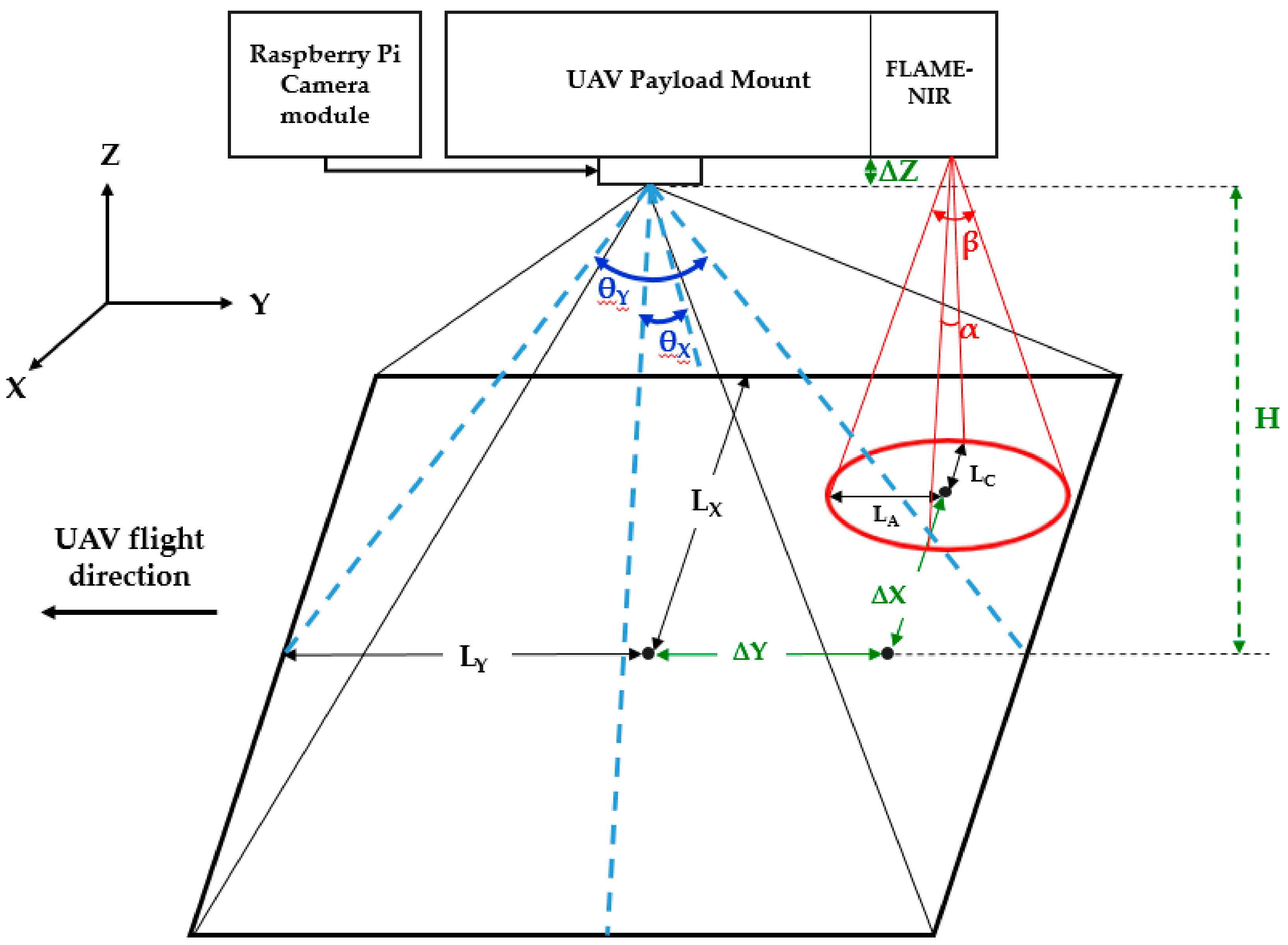
Figure 7.
Locations of the spectrometer footprints.
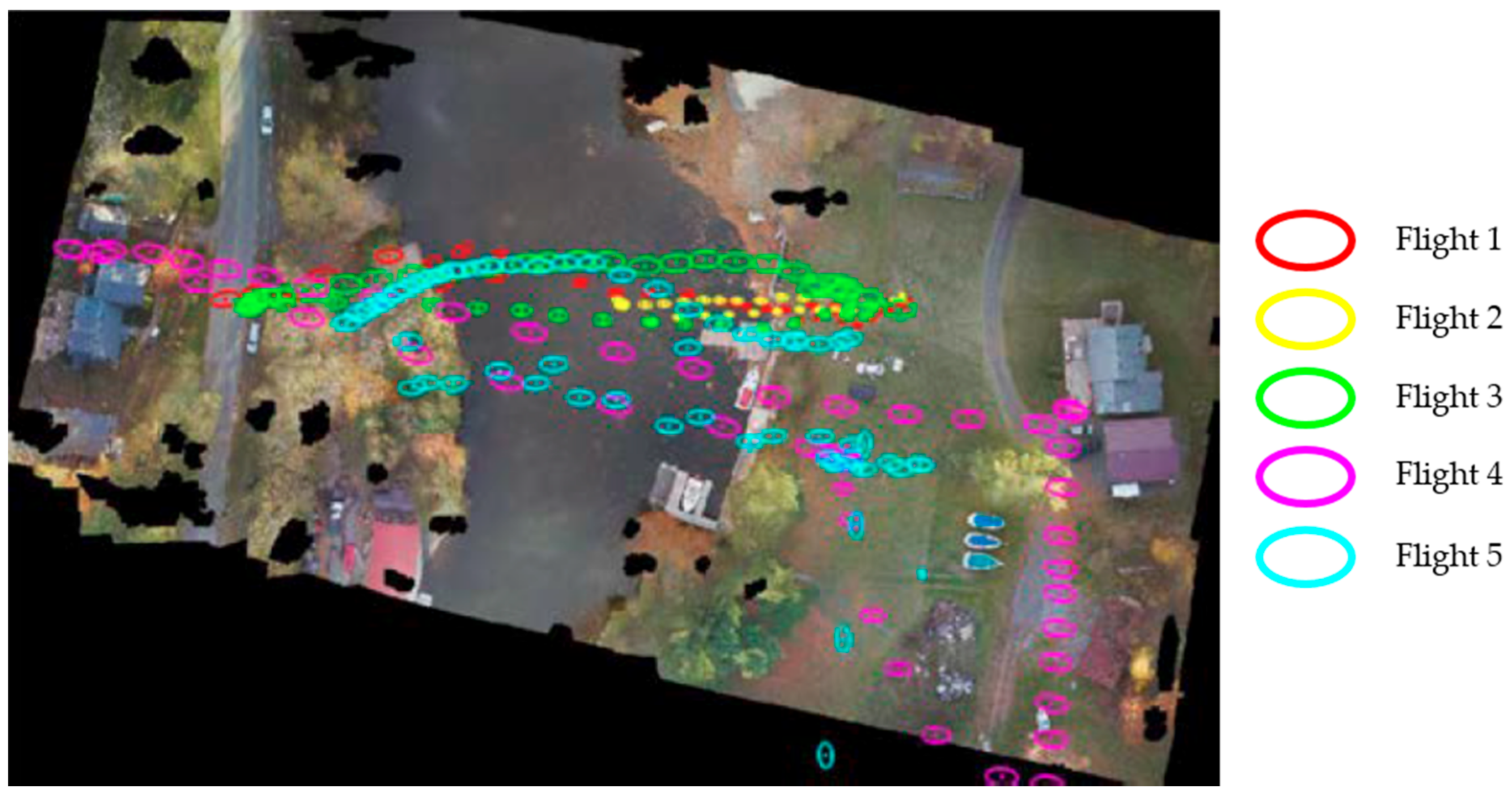
Figure 8.
Spectral Exposures of various land cover elements.

Figure 9.
Spectrometer points representing various land cover elements.

Figure 10.
Classification map produced by interpolation of labeled spectrometer points.

Figure 11.
Classification map produced by object-based image segmentation.
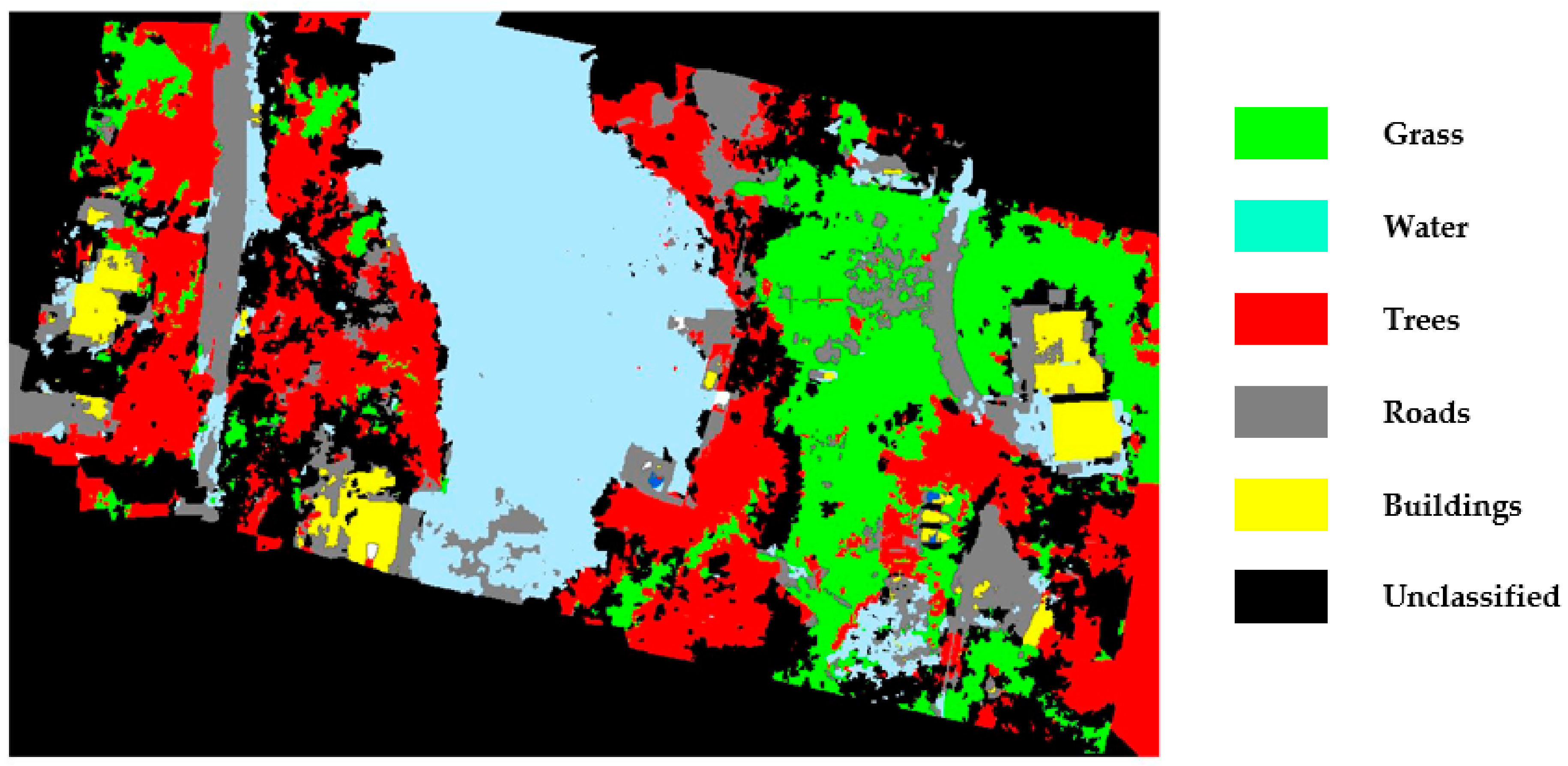
Figure 12.
Intersecting land cover classes.


Table 1.
Confusion matrix and accuracy assessment.
| Labelled Spectrometer Points | ||||||
|---|---|---|---|---|---|---|
| Truth by visual interpretation | Class | Grass | Water | Tree | Manmade | Total |
| Grass | 81 | 3 | 1 | 11 | 96 | |
| Water | 0 | 85 | 0 | 0 | 85 | |
| Tree | 8 | 2 | 18 | 5 | 33 | |
| Manmade | 13 | 4 | 1 | 23 | 41 | |
| Total | 102 | 94 | 20 | 39 | 255 | |
| Class | Grass | Water | Tree | Manmade | ||
| Errors of Omission/False negative | 15.62% | 0% | 45.45% | 43.9% | ||
| Errors of Commission/False positive | 20.59% | 9.57% | 10% | 41.02% | ||
| Overall Accuracy | 81.18% | |||||
Table 2.
Cross-tabulation of the area of intersecting classes.
| Object-Based Classification | |||||
|---|---|---|---|---|---|
| Spectrometer classification | Class | Grass (%) | Water (%) | Trees (%) | Manmade (%) |
| Grass (%) | 58 | 2 | 13 | 11 | |
| Water (%) | 0 | 78 | 10 | 6 | |
| Trees (%) | 6 | 5 | 48 | 15 | |
| Manmade (%) | 6 | 13 | 4 | 45 | |
© 2018 by the authors. Licensee MDPI, Basel, Switzerland. This article is an open access article distributed under the terms and conditions of the Creative Commons Attribution (CC BY) license (http://creativecommons.org/licenses/by/4.0/).
Share and Cite
MDPI and ACS Style
Natesan, S.; Armenakis, C.; Benari, G.; Lee, R. Use of UAV-Borne Spectrometer for Land Cover Classification. Drones 2018, 2, 16. https://doi.org/10.3390/drones2020016
AMA Style
Natesan S, Armenakis C, Benari G, Lee R. Use of UAV-Borne Spectrometer for Land Cover Classification. Drones. 2018; 2(2):16. https://doi.org/10.3390/drones2020016
Chicago/Turabian StyleNatesan, Sowmya, Costas Armenakis, Guy Benari, and Regina Lee. 2018. "Use of UAV-Borne Spectrometer for Land Cover Classification" Drones 2, no. 2: 16. https://doi.org/10.3390/drones2020016