Accuracy and Optimal Altitude for Physical Habitat Assessment (PHA) of Stream Environments Using Unmanned Aerial Vehicles (UAV)

Abstract

Physical Habitat Assessments (PHA) are useful to characterize and monitor stream and river habitat conditions, but can be costly and time-consuming. Alternative methods for data collection are getting attention, such as Unmanned Aerial Vehicles (UAV). The objective of this work was to evaluate the accuracy of UAV-based remote sensing techniques relative to ground-based PHA measurements, and to determine the influence of flight altitude on those accuracies. A UAV quadcopter equipped with an RGB camera was flown at the altitudes of 30.5 m, 61.0 m, 91.5 m and 122.0 m, and the metrics wetted width (Ww), bankfull width (Wbf) and distance to water (Dw) were compared to field PHA. The UAV-PHA method generated similar values to observed PHA values, but underestimated distance to water, and overestimated wetted width. Bankfull width provided the largest RMSE (25–28%). No systematic error patterns were observed considering the different flight altitudes, and results indicated that all flight altitudes investigated can be reliably used for PHA measurements. However, UAV flight at 61 m provided the most accurate results (CI = 0.05) considering all metrics. All UAV parameters over all altitudes showed significant correlation with observed PHA data, validating the use of UAV-based remote sensing for PHA.

1. Introduction

It is well documented that streams and rivers are negatively impacted by anthropogenic activities, including (but not limited to) agriculture, mining, forestry, energy, and transportation development. These development activities often include deforestation, pollution, channelization, expansion of impervious surfaces (e.g., roads, parking lots), and many others [1,2]. These impacts frequently result in water quality deterioration and loss of aquatic habitat [3]. Efforts in recent years to address these anthropogenic impacts to streams and rivers have generated innovative techniques to detect, characterize, and restore impaired aquatic habitats [1]. One of the most informative methods for evaluating stream and riparian condition is the Physical Habitat Assessment (PHA) [4]. PHA is based on field measurement of metrics pertaining to stream physical characteristics at intervals along the river corridor [4,5]. Physical attributes measured in PHA are related to channel dimensions, gradient and substrate, vegetation community status, habitat complexity, anthropogenic alterations, and interactions with riparian areas [6,7]. PHA provides quantitative evidence of habitat availability, types and causes of degradation, and the capacity of the channel to adjust to changes [1,4,5]. Additionally, it can be used as a tool to monitor conditions following restoration practices to evaluate success [2,3,8]. While PHA has been demonstrated to be an effective stream and riparian habitat characterization method, there remain challenges in efficiency to be addressed, particularly in projects of large spatial extent, areas of limited accessibility, and assessments requiring repeated surveys over time.

The remaining challenges in PHA are associated with data collection costs, in terms of money and time [1,4,5,9], difficulties in repeated data collection over time (i.e., replicability) [1,4,10], and accessibility of remote areas [11]. The time, and labor cost, are among the most important considerations in PHA studies, and are dependent on channel characteristics and selected variables [6]. A method for rapid physical habitat assessment in mixed-land-use watersheds was developed using field measurements and integrated GPS coordinate systems [4], and validated as a relatively fast and economical process of evaluation for restoration projects. Despite success of previous methods, both traditional and adapted PHA methods would benefit from classifications of land use information, from which the causes of degradation can be inferred [4], and additional remote-sensing-derived products and metrics [5,12], including time series of repeated measurements [13,14], mapping areas of limited access [15], evaluations in large area projects [1,16], and reductions in overall time and labor costs [5,16]. Adapting traditional PHA field techniques with remote sensing and GIS methods offers the potential to improve stream habitat characterization and monitoring through efficient collection of robust and comprehensive data.

Remote sensing techniques are becoming increasingly common in aquatic habitat assessments. Examples of such applications include: (a) use of hyperspectral and aerial imagery to map in stream habitats [17,18]; (b) optical imagery to model water depth [19]; and (c) characterization of structural stream features using LiDAR combined hyperspectral imagery [12], infra-red LiDAR [20], and vision-based photogrammetry [21]. However, these technologies are not without challenges, the most important of which is limitations in resolution necessary for accurate measurement of stream features [12,17,22]. While developments in manned, airborne high-resolution imagery and LiDAR acquisition are producing data resolutions required to support PHA metrics, the associated equipment, labor, flight, and processing costs are often prohibitively expensive, and thus limiting, particularly for smaller area projects [5,23,24]. To address these challenges, the use of Unmanned Aerial Vehicles (UAV) for remote sensing applications has become increasingly popular.

The advantages of UAV remote sensing are not limited to low costs in the acquisition of high spatial resolution imagery, but also include the ability to produce surface models (e.g., DSMs, TINs, DTMs) from the same images [14,16,23]. UAVs also offer high spectral and temporal data resolutions [5,13], a high degree of automation in the process of image acquisition and processing [14,25,26], and less influence of specific weather conditions, such as the presence of clouds that affect data collection from manned aircrafts and satellite imagery [22,27]. Moreover, many advantages of UAV imagery are related to recent developments in computer vision-based algorithms for processing. The primary source for the UAV imagery processing is called Structure from Motion (SfM). SfM is a group of algorithms that identify and track the position of features in images with overlap [28,29]. From the “movement” of these features along the images in a flight-line, SfM algorithms estimate the camera’s position and calibration parameters to reconstruct a 3D model of the scene [28,29,30,31]. UAV with SfM modeling is dependent on having requisite overlap between pictures and texture in the images that allow the recognition of features [23,32,33]. In addition, the collection of high-precision coordinates of ground control points (GCPs) are important to the accuracy of UAV SfM output [32]. Although UAV methods have great potential to overcome some of the challenges associated with other remote sensing technologies, there exist singularities and limitations of UAV methods that need to be fully understood and evaluated.

Current applications of UAV imagery in wetland and stream assessments involve feature detection/extraction to support hydrologic and hydraulic modeling, such as water depth and velocity [13]; topographic modeling of exposed and submerged stream characteristics [14,23]; and aquatic vegetation mapping [34]. Limitations of UAV imagery in PHA studies include the presence of vegetation obstructions and shadows that can obscure the view of important features [13,17]. However, these problems can be reduced with adjustments in the flight plans and use of different sensors [17,35,36]. These studies suggest benefits of UAV technology to wetland and stream assessments in general; however, the application of UAV technology to PHA, specifically, has not been completed.

Despite the recent surge of UAV imagery and SfM techniques in environmental monitoring, there remains a need for validation of the application of the method in support of PHA measurements [5]. Furthermore, there is a dearth of guidance on optimal flight parameters for effective stream measurement, such as altitude, overlap, flight direction and position, and number of ground control points. Reference [37] evaluated parameters such as flight altitude, overlap and weather conditions for application in forest structure, and observed influence of overlap and light conditions on the canopy height estimate. Reference [33] evaluated height, overlap, speed and GCP number and distribution, and noted that higher elevations provided larger errors in terms of geo-referencing. Reference [38] presented how systematic errors in the DEM due to distortions in consumer-grade cameras can be minimized by variations in flight plan, use of convergent images, different camera points of view, and variations in altitude. Yet, the results of [38] are based on simulations, and the inclusion of ground control was not completely evaluated. Reference [39] observed the importance of distributing GCPs along the vertical range of the area using three GCPs and noted reduced error when an off-nadir flight facing a cut slope was performed, in comparison with traditional nadir flights. The results from these previous works indicate that flight planning is important to the accuracy of SfM derived outputs, but parameters like overlap, altitude, view angle and others can be variable according to the application goal. Such parameters are important, because low altitudes and higher degrees of overlap require significantly longer flight times and produce larger datasets, which are more difficult to process and store [37,39]. Therefore, the optimal flight plan comprises the least amount of flight time (i.e., minimizes labor time, battery usage, weather interruptions, and poor sun angles), the smallest data volumes to be processed and analyzed, but adequate resolution to maintain the necessary level of detail. An evaluation of image acquisition parameters, and the effects of these parameters on the accuracy of remote PHA measurements, has yet to be performed.

The overarching objective of this study was to evaluate the accuracy of deriving PHA metrics from UAV imagery. A sub-objective included comparing four distinct altitudes to observed stream geomorphological measurements. The goal was to validate the use of UAV imagery and SfM methods to support PHA by reducing related field time and labor costs, while also providing an answer to one of the most important and practical questions in the application of this technology: What is the optimal relationship between flight altitude (and consequently, resolution) and measurement accuracy?

2. Materials and Methods

2.1. Study Area and Experimental Design

The investigation was conducted on the JW Ruby Research Farm (Ruby Farm) located in Reedsville, WV, USA. The Ruby Farm is owned and operated by West Virginia University located in nearby Morgantown, WV, USA (Figure 1), and consists of over 364 ha of mixed-land-use, including pasture, forests, and farming infrastructure. The current and primary use of the Ruby Farm is for beef cattle production and grazing research; however, it was historically used for horse rearing and training, and is under renovation to once again be a center for equine research and education. Ruby Run is one of several streams draining the farm and is approximately 750 m in length within the farm property, with elevations ranging from 1790 to 1692 m above sea level [40]. Ruby Run has been impacted by years of cattle grazing and removal of riparian vegetation and trees. As part of the Ruby Farm redevelopment, plans have been made for the restoration of the Ruby Run stream channel, as well as associated riparian wetlands. PHA for Ruby Run is the first step in restoration planning.

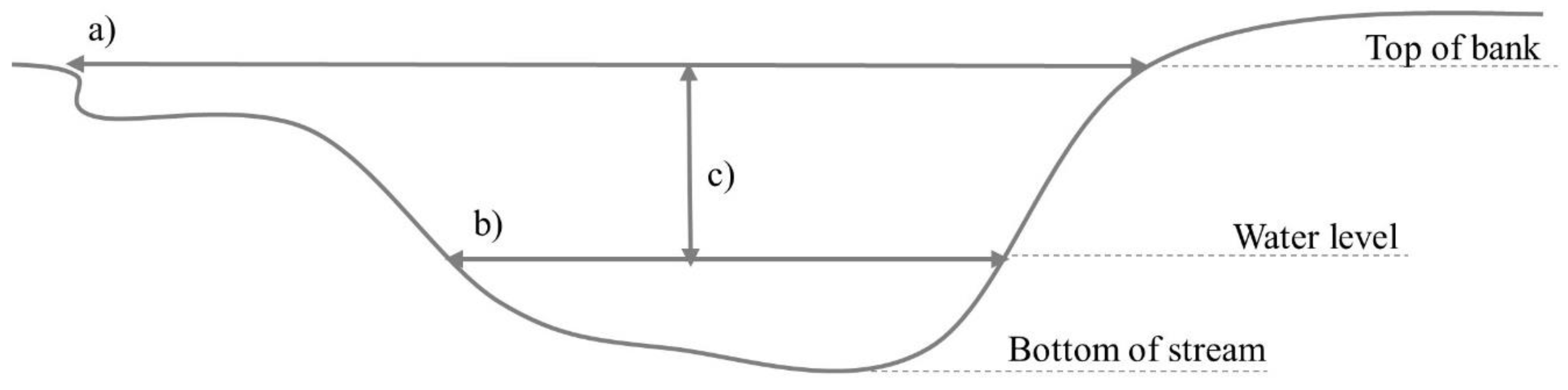
2.2. PHA Field Measurements

The PHA comprised 58 cross sections along the stream, each 10 m apart. At each cross section Wetted Width (Ww), Bankfull Width (Wbf), and Distance to Water (Dw) was physically measured by a field crew (observed data).

Bankfull width was measured as the distance at bankfull level from one bank on the other side of the channel, accomplished with an extension pole, 1.5 m level, and measuring tape. The bankfull level was identified visually by the field crew and was considered as the lowest vertical distance from the surface of the water, as described by reference [4]. Wetted width is the distance separating the points of contact between the streambank and water surface on opposite sides of the streambank and was measured using a measuring tape. Distance to water was measured using a meter stick, as the depth to bankfull from water surface. For further information pertaining to these metrics the reader is referred to [4,41] and citations within, and Figure 2. Measurements utilized the described equipment instead of GPS, given the method is simple, precise, and commonly used.

For each cross section, the initial position (every 10 m) was flagged and marked with orange paint. It is this location where channel measurements were collected.

2.3. UAV Data Collection and Processing

Aerial images were collected using a DJI Phantom 4 Professional UAV. The UAV had a RGB camera FC6310, which has 9 mm focal length, 20 MP of resolution, and 5472 × 3648 pixel array. The flights were performed using an 80% lateral and longitudinal overlap [33,42] and included a double collection flight plan, where the area is flown twice with perpendicular flight lines to increase the number of possible camera views [42,43]. The image collection was performed on the same day, at the same time as the field PHA measurements, therefore there were no differences in the creek and water level.

Image collection was completed at four altitudes: 30.5 m (100 ft), 61.0 m (200 ft), 91.5 m (300 ft), and 122.0 m (400 ft). Each altitude required at least two flights (one for each opposing flight direction). The UAV has a GPS/GNNS onboard system with accuracy of ±0.5 m horizontal and ±1.5 m vertical [44]. Despite these published nominal accuracy values, experience suggests that Phantom altitudes values are less reliable in practice, given they are calculated based on an Altitude Above Ground Level (AGL) basis as opposed to a vertical coordinate system, and they are not generated by the GNSS sensor, but rather calculated from a barometer [33].

13 painted plywood targets measuring 70 × 70 cm were distributed around the stream area before the image acquisition, to be used as ground control and check points. Accurate ground control is critical in geo-referencing images and creating SfM models, even with the presence of onboard GPS [14,32,45]. Ground control targets must be well-distributed in the interest area [33,39]. The targets’ positions were collected using a SP80 GNSS receiver using a network base RTK with horizontal and vertical accuracies of 8 and 15 mm. The network RTK was connected with the West Virginia, USA, Real Time Network, which collects information from many Continuously Operating Reference Stations (CORS) across the state. Nine plywood targets were used as ground control during the image processing (as calibration), while the other four were used as check points (validation—therefore not included in the image adjustment) to assess the positional accuracy of the processing results [33]. The position of the beginning of each field-measured cross section was also collected with the GPS, to assist locating cross section positions (i.e., field data collection points) in the imagery.

The images were processed using Agisoft Photoscan professional edition 1.3.4, used in many UAV applications with accurate results [29,46,47]. Each dataset (flight altitude) was processed separately. The processing settings were chosen based on high accuracy, since those provided more detailed geometry [29,33,47]. Images were aligned using high accuracy, and reference preselection. Ground control points were included in the model, and GCP coordinates were also used in the alignment. The dense point cloud was processed using high density and the depth filter was disabled. The DSM was created based on all the points in the dense point cloud, and the orthomosaic was created using the DSM as elevation base. The interpolation method used to create the DSM was the Inverse distance weighting (IDW). The DSM and orthomosaic resolutions were set to the highest possible for each flight altitude.

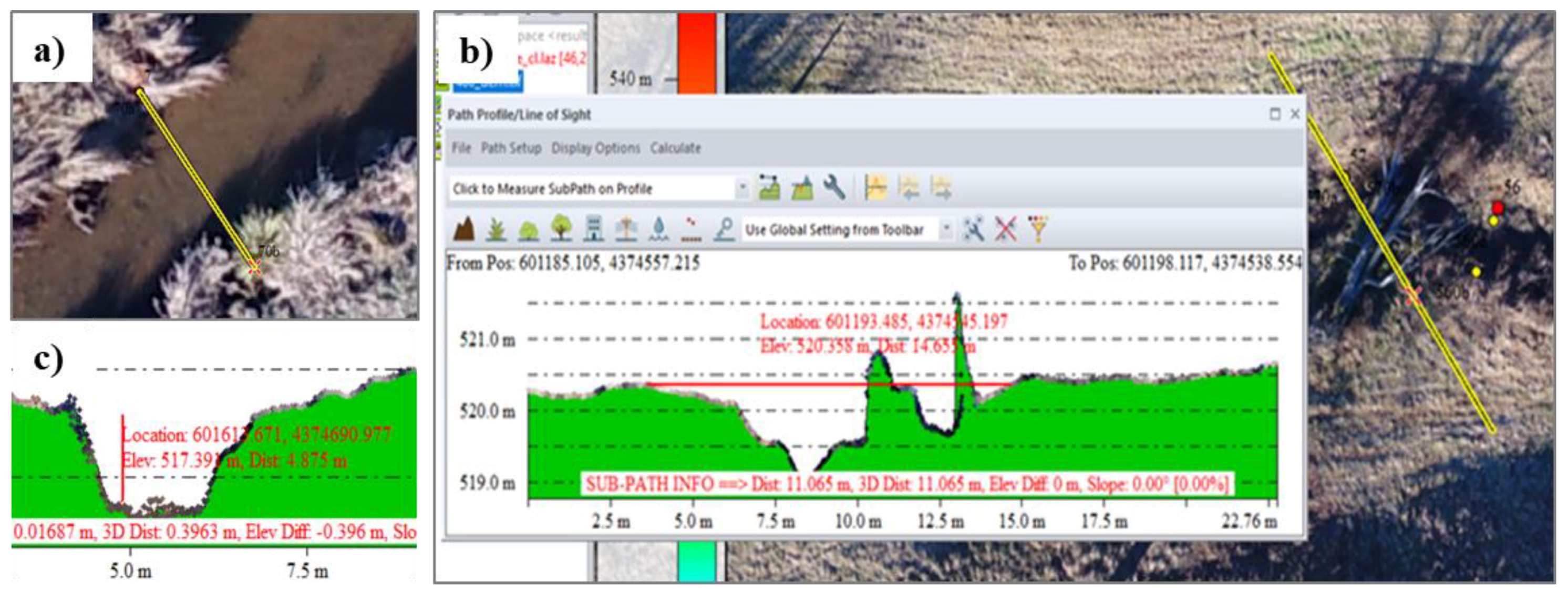
2.4. UAV PHA Measurements

Each flight altitude provided a DSM, an orthomosaic, and a 3D dense point cloud, which were used to digitally measure the same cross section dimensions as collected in the field. Each dataset was imported in Global Mapper 19 (Blue Marble Geographics, Hallowell, ME, USA), where the approximate position of the cross section was identified by the coordinate collected with the GNSS/GPS receiver.

At each stream cross section, the wetted width, bankfull width, and distance to water were digitally measured. These measurements were made based on the same metrics applied in field. However, digital observations were extracted entirely from the imagery (orthomosaic), DSM, and point cloud. To observe elevations in the cross sections, terrain profiles were created for each cross section, and the distances were measured in these profiles. Ww was visually observed in the orthomosaic, since the water was spectrally distinct from the other classes. The Wbf was identified visually in each cross-section terrain profile, considering the elevation difference and as described by reference [4]. The Dw was also manually measured in each cross-section terrain profile, as the elevation difference between bankfull and water surface, again as per reference [4] and references therein. The decision to make the measurements manually in the imagery was based on the need to adapt the current automatic methods for use in UAV-derived elevation profiles, since those are affected by vegetation presence. Therefore, the use of current, unadapted automatic methods could increase the error due to vegetation presence, which could be identified as terrain. It is less challenging to visually identify differences in elevation caused by vegetation; however, automatic methods still need to be developed.

The UAV imagery measurements required some digital processing to simulate field measurements. For example, in digitally measuring the wetted width parameter, one or both sides of the stream were often obscured by vegetation. In those cases, the exact position for the distance measurement needed to be approximated by considering nearby positions along the stream without vegetation occlusion [48]. Similarly, for bankfull width measurements, UAV-generated profiles with elevations obscured by vegetation were easily identified by analyzing the associated RGB-colored point cloud. In those cases, the elevation of vegetation or woody debris were ignored, and again, nearby positions of terrain elevations were used in the measurement. In measuring distance to water, a few outliers were observed (e.g., a few points much higher than neighboring points) and were considered noise and ignored. Therefore, the distance to water is an approximation, since it is unknown whether the point cloud is reflecting the water surface or the stream bottom (Figure 3).

Since the UAV PHA measurements were made manually, each dataset (flight altitude) took approximately 5–6 h to be completed. Besides this process being time consuming, it is important to note that the timing depends on the experience of the person performing the manual measurements, and that this could be automatized in a future process.

2.5. Statistical Analysis

Statistical analyses were performed to compare PHA observed values with the UAV digital estimations, considering the wetted width, bankfull width, and distance to water metrics. Furthermore, UAV estimates were compared to observed (measured) data according to the different flight altitudes.

Statistical analyses included generating descriptive statistics of observed and UAV altitude (n = 4) comparative measurements (i.e., bankfull width, wetted width, distance to water), calculating the Root Mean Square Error (RMSE) and Spearman’s correlation coefficient, and via a graphical analysis of the values. The RMSE is calculated as follows (Equation (1)).

$$\mathrm{RMSE}\left(\mathrm{m}\right)=\sqrt{\frac{{\sum }_{\mathrm{i}=1}^{\mathrm{n}}{\left({\mathrm{y}}_{\mathrm{i}}-{\mathrm{x}}_{\mathrm{i}}\right)}^2}{\mathrm{n}}},$$

(1)

where: ${\mathrm{y}}_{\mathrm{i}}$ and ${\mathrm{x}}_{\mathrm{i}}$ are the measured variable in the field and in the UAV data, respectively; n is the number of observations.

Spearman’s correlation coefficient is a non-parametric method to measure the strength of the relationship between two variables [49]. The correlation was calculated using the software R [50] and the package pspearman [51].

3. Results

3.1. UAV Products

Each of the four flight altitudes provided distinct parameters (

Table 1. Data acquisition and processing.

Flight Altitude (m)	Pictures (n)	Area (km2) 1	Resolution (cm/pix)		Density (points/m2)	Time (h:m) 2
			Ortho	DSM		Processing	Flight
122.0	100	0.156	3.13	6.25	256	4:01	0:16
91.5	158	0.125	2.31	4.62	468	7:01	0:20
61.0	364	0.0996	1.54	3.08	105,000	16:22	0:31
30.5	828	0.0587	0.786	1.57	404,000	33:15	1:07

¹ the area refers to the surface covered by all the images together. ² the processing time only includes the processing performed in Agisoft Photoscan.

). As anticipated, the number of images increased exponentially at lower altitudes. Yet, as the number of images increased, the covered area decreased. The higher altitude pictures have a larger footprint, and thus, cover a larger extent individually [52,53,54].

The resolution of the orthomosaic and DSM increased with the lower altitudes, with the lowest flight (30.5 m) displaying approximately four times more detail than the highest flight (122 m). The point density also increased in the lower altitudes, with more than 400 thousand points per m² in the 30.5 m flight. However, the processing time practically doubled with each reduction in altitude. Flight time also increased substantially in the lowest altitude flight, probably because at this altitude it was necessary to perform two flights in each direction to complete the mission, necessitating a total of four flights at the 30.5 m altitude, while the other three altitudes required only two.

The positional accuracy of each flight altitude was also recorded (

Table 2. Geolocation RMSE errors based on the check points.

Flight Altitude (m)	X (cm)	Y (cm)	Z (cm)	Absolute Error (cm)
122.0	2.12	0.43	2.49	3.30
91.5	1.67	1.01	1.98	2.78
61.0	1.94	1.00	3.08	3.77
30.5	1.05	1.41	2.97	3.45

). There was no clear influence of flight altitude on this parameter. The largest errors were observed in the Z coordinate, and the maximum error total observed was 3.77 cm for the 61 m flight. Therefore, all flight heights obtained an adequate positional accuracy.

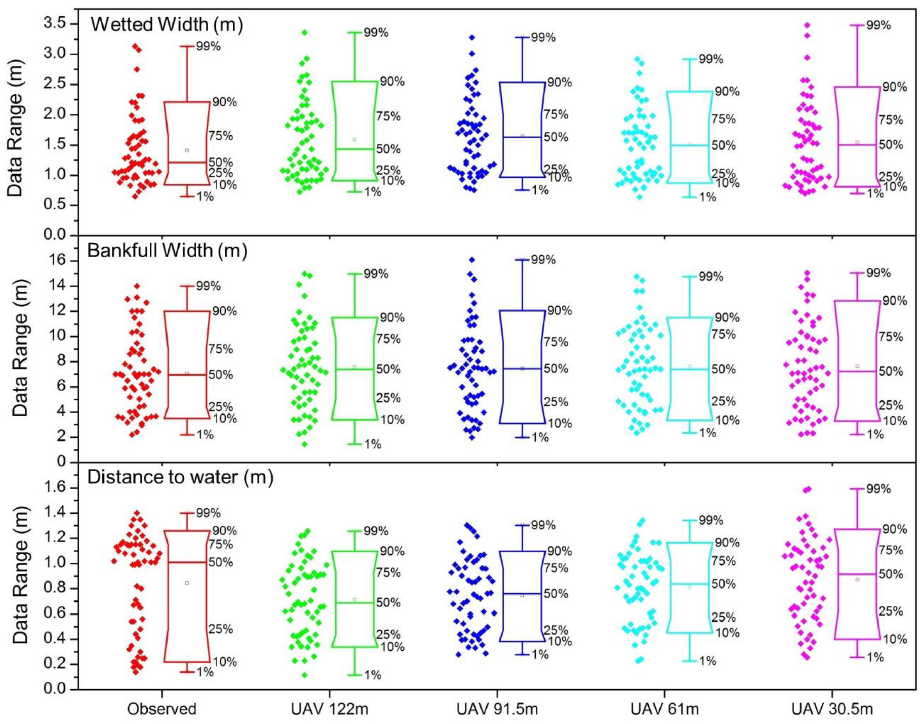
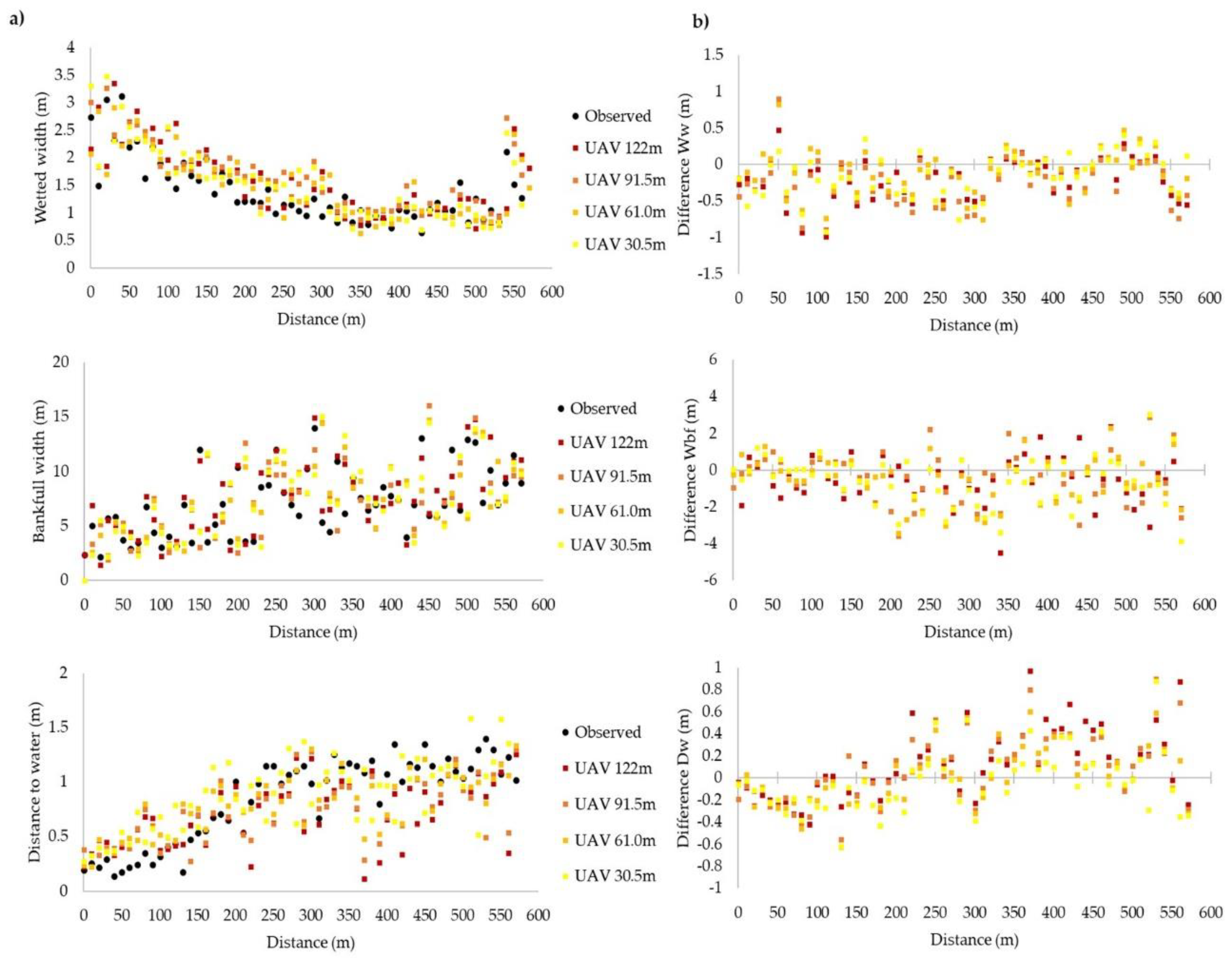
3.2. Observed and UAV Data Description

One orthomosaic, one DSM, and one 3D dense point cloud were generated from each flight altitude and used in the UAV digital cross section measurements. Descriptive statistics for the metrics measured are presented in

Table 3. Descriptive Physical Habitat Assessments (PHA) statistics of wetted width, bankfull width and distance to water from the PHA and UAV measurements.

Statistic	Observed	UAV 122.0 m	UAV 91.5 m	UAV 61.0 m	UAV 30.5 m
	Wetted Width (m)
Mean	1.41	1.59	1.64	1.51	1.54
Maximum	3.13	3.36	3.28	2.92	3.48
Minimum	0.65	0.73	0.76	0.64	0.70
Median	1.21	1.43	1.63	1.49	1.50
SD	0.56	0.63	0.61	0.58	0.67
	Bankfull Width (m)
Mean	7.07	7.58	7.43	7.62	7.65
Maximum	14.00	14.97	16.08	14.75	15.05
Minimum	2.20	1.46	1.98	2.35	2.22
Median	6.96	7.39	7.44	7.40	7.23
SD	3.08	3.22	3.37	3.19	3.42
	Distance to Water (m)
Mean	0.84	0.71	0.75	0.81	0.87
Maximum	1.40	1.26	1.30	1.34	1.59
Minimum	0.14	0.12	0.28	0.23	0.26
Median	1.01	0.69	0.76	0.84	0.91
SD	0.39	0.29	0.28	0.27	0.33

. Wetted and bankfull width UAV measurements displayed a larger range than the observed data, except for the 61 m UAV flight (Figure 4). In both UAV and observed data, some points were observed above the 90% percentile. For wetted width, it is important to note that the observed values were concentrated below the mean (i.e., right-skewed), while the UAV data showed a more even distribution. For bankfull width, the distribution of UAV and observed data was similar. Distance to water showed the largest difference between UAV and observed data distributions, with observed data displaying left-skewness and UAV data well-distributed across the range. For wetted width, the majority of UAV data points were overestimations, relative to observed values, yet the values were similar. Bankfull width presented a similar tendency, but the UAV method estimated lower minimum values in some cases. For distance to water, most UAV data points comprised underestimations, relative to observed values, although results of the 30.5 m altitude flight indicated slight overestimation.

The relationship between field-measured values and UAV measurements along the stream corridor are presented in Figure 5. The figure further illustrates overestimation of wetted width by UAV measurements, while distance to water was generally underestimated. Wetted width displayed larger values upstream, generally decreasing downstream, excepting the cross sections at the end of the corridor. Distance to water showed the opposite trend, with values consistently increasing downstream. Bankfull width exhibited small values at the beginning of the stream corridor, with the rest of the corridor presenting a larger range of values. Collectively, longitudinal patterns of measured metrics indicate a representative incised (decreasing wetted width, increasing depth to water) stream, consistent with results from previous PHAs conducted on streams subject to agricultural land uses [41]. Importantly, parameter values estimated by the UAV method did not exhibit consistent overestimation or underestimation, or systematic increases or decreases in accuracy with changes in altitude.

3.3. Statistical Comparison

Table 4. RMSE and Spearman’s correlation coefficient between observed and UAV data for wetted width, bankfull width and distance to water.

Value 1	Value 2	RMSE (m)	RMSE (%)	SCC
		Wetted Width
Observed	UAV 122.0 m	0.34	7.99	0.90 *
Observed	UAV 90.5 m	0.39	10.79	0.88 *
Observed	UAV 61.0 m	0.32	7.09	0.85 *
Observed	UAV 30.5 m	0.32	7.29	0.87 *
		Bankfull Width
Observed	UAV 122.0 m	1.33	25.01	0.92 *
Observed	UAV 90.5 m	1.38	26.83	0.91 *
Observed	UAV 61.0 m	1.33	25.00	0.93 *
Observed	UAV 30.5 m	1.42	28.70	0.93 *
		Distance to water
Observed	UAV 122.0 m	0.34	13.35	0.59 *
Observed	UAV 90.5 m	0.31	11.54	0.62 *
Observed	UAV 61.0 m	0.27	8.37	0.67 *
Observed	UAV 30.5 m	0.27	8.61	0.66 *

SCC: Spearman’s correlation coefficient; * significant correlation at 95% probability.

presents RMSE values between observed and UAV data for each metric, as well the correlation. Wetted width was the metric with the lowest error, ranging from 7.1–10.8% RMSE, while bankfull width showed the largest error, ranging from 25.0–28.7% RMSE. UAV estimates of both wetted and bankfull widths displayed high correlation with observed values (SCC ≥ 0.85). Despite differences, error and correlations were not strongly influenced by flight altitude for wetted and bankfull widths. Distance from water showed the largest variation between the different UAV flight altitudes and showed smaller error in the two lowest flights. However, correlations of observed and UAV data were statistically significant (p < 0.05).

4. Discussion

Collectively, results of the current work highlight the utility of UAV imagery for PHA. From this imagery, high spatial resolution data can be obtained to generate spectral and 3D information for efficient and cost-effective aquatic habitat measurements, even at the highest flight altitudes permitted by US FAA. The lowest spatial resolution generated was 3 cm for the orthomosaic and 6 cm for the DSM at the highest flight altitude, which required only 16 min of flight time and 4 h of processing time. It is important to note that similar conclusions were observed in related works [23,34]. Also, the UAV geolocation accuracy observed in this research was high, compared to other studies [33,53], and a relationship between positional error and flight altitude as observed in other studies was not detected [33,37,53]. This validates the method of acquisition in this study as reliable (in terms of flight-line overlap, GCP number and position, UAV and GNSS sensors applied).

UAV-estimated PHA values have a similar trend to values observed via traditional methods. In general, UAV data displayed a similar distribution to field measurements. However, UAV data were characterized by a larger range, which may be due to slight differences in measurement positions to adjust for vegetation and woody debris in the digital data. Bankfull width displayed large RMSE values. However, considering high observed correlations between UAV and observed values (SCC > 0.9), error could likely be improved in the future via more stringent data post-processing and methodological refinement. Notably, RMSE values were not strongly influenced by flight altitude, suggesting errors were not related to spatial resolution for this parameter. Importantly, the lack of altitude impact on UAV estimate accuracy suggests that increased expenditures in terms of labor (e.g., flight time, data processing requirements) associated with lower altitude UAV flights may not produce more accurate estimations of stream physical parameters, and thus are likely not justified.

Given point clouds used in generating DSMs included all surface features, such as tall grass and shrubs, Wbf and Ww error could also be attributable to the presence of vegetation and occlusions caused by shadows [13,48,55]. Vegetation interference is one of the main sources of error in digital models derived from UAV imagery [13,23], whereas in areas with no vegetation it is possible to obtain DSMs with comparable precision to LiDAR [23]. Reference [55] notes the possibility of classifying and excluding vegetation by interpolating from adjacent cells, but this process may introduce large errors if adjacent cells are not in the same plane (e.g., channel edges). Shadows are known to interfere in both radiometric image aspect [56,57] and 3D reconstruction [58], and comprise a challenge to the detection of match points in the alignment process [36,59].

The distance to water parameter showed the lowest correlations and RMSE values between observed and UAV estimated values. For distance to water, it was also observed that most of the errors were underestimates, a common problem in remotely sensing streams [13,14]. A primary source of this error stems from differential refraction of light between air and water which affects water depth and topographic measurements in submerged areas [13,14,55]. References [14,55] observed larger error in the DSM with increasing water depth. This may explain smaller differences in distance to water values between observed and UAV measurements in shallower, upstream segments of the reach in the current work. Also, distance to water errors could be related to problems in the photogrammetric reconstruction of areas with water in the surface, since the reflection of the water can present challenges finding matches in the SfM algorithms due to the presence of low texture in deep water, sun reflection, and water turbidity [21,23,54]. Lastly, errors in the distance to water measurement may be related to erroneous measurements in the bankfull width from which they are derived. Difficulties encountered in estimating distance to water provide impetus for continued work regarding the refinement of UAV PHA methodology.

Despite differences between UAV and field-observed bankfull width, it is possible that UAV estimates are more precise, given the comprehensive 3D view of the stream corridor on which they are based, and which may facilitate the visual recognition of channel limits difficult to spot in the field. Moreover, unlike PHA reliance on a discrete and limited number of cross sectional observations, UAV data provides information for the entire stream reach, affording essentially limitless cross sectional data for analysis [20]. Data collected by UAVs are versatile, supporting a variety of stream-based surveys in addition to or in combination with PHA, including hydrologic and hydraulic modeling, stream restoration design, flood mapping, and planning for fish habitat improvements [13,17,19,23]. While current UAV technology may be most useful in small study areas [23,34], results of the current work confirm that UAV data collected at even the highest legal altitudes offer an efficient and effective alternative to traditional methods of PHA data collection.

It is important to consider that there are additional options to perform PHA measurements, such as the use of GPS presented in [4,41]. The use of GPS to measure the metrics evaluated in this study would require four positions for each cross section (both limit sides of bankfull, and both limits of wetted area). In the current study, the collection of one position in each cross section took approximately 2 h, therefore it is reasonable to expect that the collection of four points would take at least twice as long (since there is no need to walk between points in the same cross section). Thus, for the experimental stream reach of approximately 750 m, the GPS collection could take approximately four hours, although the time would also be constrained by the number of individuals in the field crew. Therefore, the data collection process may take more than four hours, while the image collection with the highest flight altitude took only 16 min and needed approximately 4 h of processing (in office, and mostly for computational time without the need of supervision). This difference in time would be more significant in larger areas, or in streams with limited access. Despite the need for a few additional ground control points in larger projects, the UAV approach would clearly outpace traditional or GPS field measurement over larger project areas, yet UAV are may not be the most cost efficient for very larger areas, where manned aircrafts or high-resolution satellites could be the recommended choice [60]. In addition to speed and ease of data collection and processing, UAV data can be analyzed in office, with a full 3D view of the area, to detect bankfull edges in as many positions as needed, data which can also be used as an archive of stream condition for future reference.

5. Conclusions

The current work evaluated the viability of using UAV-derived imagery to simulate PHA field measurements. The main objective was to estimate the accuracy of UAV-based remote sensing methods in comparison to traditional measurements, as well to understand the effect of different flight altitudes on the accuracy of UAV PHA measurements.

Results indicated UAV PHA values present a similar trend as the observed PHA metrics used in the current work. In general, the UAV method overestimated wetted width while underestimating distance to water. Yet, bankfull width presented the largest errors, as illustrated by RMSE values. Differences between observed and UAV PHA values are likely related to problems in the correct characterization of the metrics in the imagery, since it was performed manually, and to limitations of the UAV system applied. Therefore, results from the UAV PHA were considered valid, highlighting the applicability of the method for stream research in general, and physical habitat assessments specifically. The UAV flight altitudes showed differences in accuracy, relative to observed values, but differences were not characterized by a systematic relationship, which emphasizes the utility of even the highest legal flight altitude in the USA (FAA regulations) for PHA studies. Although the flight at 61.0 m aboveground provided the best results, the highest flight altitude provided similar results, and can therefore be recommended since it allows faster data collection and processing.

Future studies should evaluate other UAV planning/flight variables, such as photo overlap percentage (80% forward, 80% side was held constant in this study), flight directions, and number and placement of ground control points, given these parameters also impact UAV data collection and processing time. Data processing parameters could be modified to lower settings to reduce processing time and file sizes, and many other PHA metrics should be validated. Future work should address the development of an automated method to detect and measure PHA metrics in UAV outputs, considering the manual identification (as performed in the current study) was labor intensive and time consuming.

Collectively, results illustrate the value of UAV-based remote sensing techniques for the characterization of stream habitat conditions. Considering the reduced time and labor associated with UAV methods, as compared to traditional field-based approaches, results support the adoption of UAV methods for routine physical habitat assessment, which can in turn improve outcomes of land and water resource management strategies and more effectively target restoration and remediation efforts at reduced costs.

References

1. Maddock, I. The importance of physical habitat assessment for evaluating river health. Freshw. Biol. 1999, 41, 373–391. [Google Scholar] [CrossRef]
2. Violin, C.R.; Cada, P.; Sudduth, E.B.; Hassett, B.A.; Penrose, D.L.; Bernhardt, E.S. Effects of urbanization and urban stream restoration on the physical and biological structure of stream ecosystems. Ecol. Appl. 2011, 21, 1932–1949. [Google Scholar] [CrossRef] [PubMed]
3. Davis, N.M.; Weaver, V.; Parks, K.; Lydy, M.J. An assessment of water quality, physical habitat, and biological integrity of an urban stream in Wichita, Kansas, prior to restoration improvements (Phase I). Arch. Environ. Contam. Toxicol. 2003, 44, 351–359. [Google Scholar] [CrossRef] [PubMed]
4. Hooper, L.; Hubbart, J. A Rapid Physical Habitat Assessment of Wadeable Streams for Mixed-Land-Use Watersheds. Hydrology 2016, 3, 37. [Google Scholar] [CrossRef]
5. Hubbart, J.; Kellner, E.; Kinder, P.; Stephan, K. Challenges in Aquatic Physical Habitat Assessment: Improving Conservation and Restoration Decisions for Contemporary Watersheds. Challenges 2017, 8, 31. [Google Scholar] [CrossRef]
6. Peck, D.V.; Herlihy, A.T.; Hill, B.H.; Hughes, R.M.; Kaufmann, P.R.; Klemm, D.J.; Lazorchak, J.M.; McCormick, F.H.; Peterson, S.A.; Ringold, P.L.; et al. (Eds.) Environmental Monitoring and Assessment Program—Surface Waters Western Pilot Study: Field Operations Manual for Wadeable Streams; EPA/620/R-06/003; U.S. Environmental Protection Agency: Washington, DC, USA, 2006; 248p.
7. Kaufmann, P.R. Physical Habitat. In Stream Indicator and Design Workshop; Hughes, R.M., Ed.; U.S. Environmental Protection Agency: Corvalis, OR, USA, 1993; pp. 59–69. [Google Scholar]
8. Elliot, C.R.N.; Dunbar, M.J.; Gowing, I.; Acreman, M.C. A habitat assessment approach to the management of groundwater dominated rivers. Hydrol. Process. 1999, 13, 459–475. [Google Scholar] [CrossRef]
9. Harding, J.; Clapcott, J.; Quinn, J.; Hayes, J.; Joy, M.; Storey, R.; Greig, H.; Hay, J.; James, T.; Beech, M.; et al. Stream Habitat Assessment Protocols for Wadeable Rivers and Streams of New Zealand; School of Biological Sciences, University of Canterbury: Christchurch, New Zealand, 2009; ISBN 9780473151515. [Google Scholar]
10. Thomson, J.R.; Taylor, M.P.; Fryirs, K.A.; Brierley, G.J. A geomorphological framework for ri7er characterization and habitat assessment. Aquat. Conserv. Mar. Freshw. Ecosyst. 2001, 11, 373–389. [Google Scholar] [CrossRef]
11. Acreman, M.C.; Booker, D.J.; Goodwin, T.H.; Dunbar, M.J.; Maddock, I.; Hardy, T.; Rivas-Casado, M.; Young, A.; Gowing, I.M. Rapid Assessment of Physical Habitat Sensitivity to Abstraction (RAPHSA); Environment Agency: Bristol, UK; Center for Ecology and Hydrology: Oxfordshire, UK, 2008; ISBN 9781844328987.
12. Hall, R.K.; Watkins, R.L.; Heggem, D.T.; Jones, K.B.; Kaufmann, P.R.; Moore, S.B.; Gregory, S.J. Quantifying structural physical habitat attributes using LIDAR and hyperspectral imagery. Environ. Monit. Assess. 2009, 159, 63–83. [Google Scholar] [CrossRef] [PubMed]
13. Tamminga, A.; Hugenholtz, C.; Eaton, B.; Lapointe, M. Hyperspatial Remote Sensing of Channel Reach Morphology and Hydraulic Fish Habitat Using an Unmanned Aerial Vehicle (UAV): A First Assessment in the Context of River Research and Management. River Res. Appl. 2015, 31, 379–391. [Google Scholar] [CrossRef]
14. Woodget, A.S.; Carbonneau, P.E.; Visser, F.; Maddock, I.P. Quantifying submerged fluvial topography using hyperspatial resolution UAS imagery and structure from motion photogrammetry. Earth Surf. Process. Landf. 2015, 40, 47–64. [Google Scholar] [CrossRef]
15. Lee, T.M.; Yeh, H.C. Applying remote sensing techniques to monitor shifting wetland vegetation: A case study of Danshui River estuary mangrove communities, Taiwan. Ecol. Eng. 2009, 35, 487–496. [Google Scholar] [CrossRef]
16. Javernick, L.; Brasington, J.; Caruso, B. Modeling the topography of shallow braided rivers using Structure-from-Motion photogrammetry. Geomorphology 2014, 213, 166–182. [Google Scholar] [CrossRef]
17. Perschbacher, J. The Use of Aerial Imagery to Map In-Stream Physical Habitat Related to Summer Distribution of Juvenile Salmonids in a Southcentral Alaskan Stream. Master’s Thesis, University of Alaska Fairbanks, Fairbanks, AK, USA, 2011. [Google Scholar]
18. Marcus, W.A.; Legleiter, C.J.; Aspinall, R.J.; Boardman, J.W.; Crabtree, R.L. High spatial resolution hyperspectral mapping of in-stream habitats, depths, and woody debris in mountain streams. Geomorphology 2003, 55, 363–380. [Google Scholar] [CrossRef]
19. Fonstad, M.A.; Marcus, W.A. Remote sensing of stream depths with hydraulically assisted bathymetry (HAB) models. Geomorphology 2005, 72, 320–339. [Google Scholar] [CrossRef]
20. Faux, R.N.; Buffington, J.M.; Whitley, M.G.; Lanigan, S.H.; Roper, B.B. Use of airborne near-infrared LiDAR for determining channel cross-section characteristics and monitoring aquatic habitat in Pacific Northwest rivers: A preliminary Analysis. In PNAMP Special Publication: Remote Sensing Applications for Aquatic Resource Monitoring; Bayer, J.M., Schei, J.L., Eds.; Pacific Northwest Aquatic Monitoring Partnership: Cook, WA, USA, 2009; pp. 43–60. [Google Scholar]
21. Dietrich, J.T. Riverscape mapping with helicopter-based Structure-from-Motion photogrammetry. Geomorphology 2016, 252, 144–157. [Google Scholar] [CrossRef]
22. Marcus, W.A. Remote sensing of the hydraulic environment in gravel bed rivers. In Gravel-Bed Rivers: Processes, Tools, Environments; Church, M., Biron, P.M., Roy, A.G., Eds.; John Wiley & Sons, Ltd.: Chichester, West Sussex, UK, 2010; pp. 261–285. [Google Scholar]
23. Fonstad, M.A.; Dietrich, J.T.; Courville, B.C.; Jensen, J.L.; Carbonneau, P.E. Topographic structure from motion: A new development in photogrammetric measurement. Earth Surf. Process. Landf. 2013, 38, 421–430. [Google Scholar] [CrossRef]
24. Mancini, F.; Dubbini, M.; Gattelli, M.; Stecchi, F.; Fabbri, S.; Gabbianelli, G. Using unmanned aerial vehicles (UAV) for high-resolution reconstruction of topography: The structure from motion approach on coastal environments. Remote Sens. 2013, 5, 6880–6898. [Google Scholar] [CrossRef] [Green Version]
25. Koutsoudis, A.; Vidmar, B.; Arnaoutoglou, F. Performance evaluation of a multi-image 3D reconstruction software on a low-feature artefact. J. Archaeol. Sci. 2013, 40, 4450–4456. [Google Scholar] [CrossRef]
26. Lisein, J.; Michez, A.; Claessens, H.; Lejeune, P. Discrimination of deciduous tree species from time series of unmanned aerial system imagery. PLoS ONE 2015, 10, e0141006. [Google Scholar] [CrossRef] [PubMed] [Green Version]
27. Salamí, E.; Barrado, C.; Pastor, E. UAV flight experiments applied to the remote sensing of vegetated areas. Remote Sens. 2014, 6, 11051–11081. [Google Scholar] [CrossRef] [Green Version]
28. Quan, L. Image Based Modeling; Springer: New York, NY, USA, 2010; ISBN 9781441966780. [Google Scholar]
29. Verhoeven, G. Taking computer vision aloft—Archaeological three-dimensional reconstructions from aerial photographs with photoscan. Archaeol. Prospect. 2011, 62, 61–62. [Google Scholar] [CrossRef]
30. Fisher, R.B.; Breckon, T.P.; Dawson-Howe, K.; Fitzgibbon, A.; Robertson, C.; Trucco, E.; Williams, C.K.I. Dictionary of Computer Vision and Image Processing, 2nd ed.; John Wiley & Sons Ltd.: Chichester, West Sussex, UK, 2014. [Google Scholar]
31. Szeliski, R. Structure from Motion. In Computer Vision Algorithms and Applications; Szeliski, R., Ed.; Springer: London, UK, 2011; pp. 303–334. [Google Scholar]
32. Nex, F.; Remondino, F. UAV for 3D mapping applications: A review. Appl. Geomat. 2014, 6, 1–15. [Google Scholar] [CrossRef]
33. Raczynski, R.J. Accuracy Analysis of Products Obtained from UAV-Borne Photogrammetry Influenced by Various Flight Parameters. Master Thesis, Norwegian University of Science and Technology, Trondheim, Norway, 2017. [Google Scholar]
34. Husson, E.; Hagner, O.; Ecke, F. Unmanned aircraft systems help to map aquatic vegetation. Appl. Veg. Sci. 2014, 17, 567–577. [Google Scholar] [CrossRef]
35. Lehmann, J.R.K.; Nieberding, F.; Prinz, T.; Knoth, C. Analysis of unmanned aerial system-based CIR images in forestry-a new perspective to monitor pest infestation levels. Forests 2015, 6, 594–612. [Google Scholar] [CrossRef] [Green Version]
36. Wallace, L.; Lucieer, A.; Malenovsky, Z.; Turner, D.; Vopenka, P. Assessment of forest structure using two UAV techniques: A comparison of airborne laser scanning and structure from motion (SfM) point clouds. Forests 2016, 7, 62. [Google Scholar] [CrossRef]
37. Dandois, J.P.; Olano, M.; Ellis, E.C. Optimal altitude, overlap, and weather conditions for computer vision uav estimates of forest structure. Remote Sens. 2015, 7, 13895–13920. [Google Scholar] [CrossRef]
38. James, M.R.; Robson, S. Mitigating systematic error in topographic models derived from UAV and ground-based image networks. Earth Surf. Process. Landf. 2014, 39, 1413–1420. [Google Scholar] [CrossRef]
39. Carvajal-Ramírez, F.; Agüera-Vega, F.; Martínez-Carricondo, P.J. Effects of image orientation and ground control points distribution on unmanned aerial vehicle photogrammetry projects on a road cut slope. J. Appl. Remote Sens. 2016, 10, 34004. [Google Scholar] [CrossRef]
40. West Virginia GIS Technical Center (WVGISTC). Digital Elevation Models (USGS 3-Meter). 2003. Available online: http://wvgis.wvu.edu/data/dataset.php?ID=261 (accessed on 12 March 2018).
41. Hooper, L. A Stream Physical Habitat Assessment in an Urbanizing Watershed of the Central U.S.A. Master’s Thesis, University of Missouri-Columbia, Columbia, MO, USA, 2015. [Google Scholar]
42. Pix4D Designing the Image Acquisition Plan. Available online: https://support.pix4d.com/hc/en-us/articles/202557459 (accessed on 12 March 2018).
43. Röder, M.; Hill, S.; Latifi, H. Best Practice Tutorial: Technical Handling of the UAV “DJI Phantom 3 Professional” and Processing of the Acquired Data; Technical Report; University of Würzburg: Würzburg, Germany, 2017. [Google Scholar]
44. DJI Phantom 4 Specs. Available online: https://www.dji.com/phantom-4/info (accessed on 12 March 2018).
45. Küng, O.; Strecha, C.; Beyeler, A.; Zufferey, J.-C.; Floreano, D.; Fua, P.; Gervaix, F. the Accuracy of Automatic Photogrammetric Techniques on Ultra-Light UAV Imagery. ISPRS Int. Arch. Photogramm. Remote Sens. Spat. Inf. Sci. 2011, XXXVIII-1, 125–130. [Google Scholar] [CrossRef]
46. Sona, G.; Pinto, L.; Pagliari, D.; Passoni, D.; Gini, R. Experimental analysis of different software packages for orientation and digital surface modelling from UAV images. Earth Sci. Inform. 2014, 7, 97–107. [Google Scholar] [CrossRef]
47. Jaud, M.; Passot, S.; Le Bivic, R.; Delacourt, C.; Grandjean, P.; Le Dantec, N. Assessing the accuracy of high resolution digital surface models computed by PhotoScan and MicMac in sub-optimal survey conditions. Remote Sens. 2016, 8. [Google Scholar] [CrossRef]
48. Niedzielski, T.; Witek, M.; Spallek, W. Observing river stages using unmanned aerial vehicles. Hydrol. Earth Syst. Sci. 2016, 20, 3193–3205. [Google Scholar] [CrossRef]
49. Hauke, J.; Kossowski, T. Comparison of values of pearson’s and spearman’s correlation coefficients on the same sets of data. Quaest. Geogr. 2011, 30, 87–93. [Google Scholar] [CrossRef]
50. R Core Team. R: A Language and Environment for Statistical Computing; R Foundation for Statistical Computing: Vienna, Austria, 2016. [Google Scholar]
51. Savicky, P. pspearman: Spearman’s Rank Correlation Test. 2014. Available online: https://cran.r-project.org/web/packages/pspearman/pspearman.pdf (accessed on 12 March 2018).
52. Chao, H.; Chen, Y. Remote Sensing and Actuation Using Unmanned Vehicles; John Wiley & Sons, Inc.: Hoboken, NJ, USA, 2012; ISBN 9781118377178. [Google Scholar]
53. Mesas-Carrascosa, F.J.; García, M.D.N.; De Larriva, J.E.M.; García-Ferrer, A. An analysis of the influence of flight parameters in the generation of unmanned aerial vehicle (UAV) orthomosaicks to survey archaeological areas. Sensors 2016, 16. [Google Scholar] [CrossRef] [PubMed]
54. Westaway, R.M.; Lane, S.N.; Hicks, D.M. Remote survey of large-scale braided, gravel-bed rivers using digital photogrammetry and image analysis. Int. J. Remote Sens. 2003, 24, 795–815. [Google Scholar] [CrossRef]
55. Bird, S.; Hogan, D.; Schwab, J. Photogrammetric monitoring of small streams under a riparian forest canopy. Earth Surf. Process. Landf. 2010, 35, 952–970. [Google Scholar] [CrossRef]
56. Casado, M.R.; Gonzalez, R.B.; Kriechbaumer, T.; Veal, A. Automated identification of river hydromorphological features using UAV high resolution aerial imagery. Sensors 2015, 15, 27969–27989. [Google Scholar] [CrossRef] [PubMed] [Green Version]
57. Näsi, R.; Honkavaara, E.; Lyytikäinen-Saarenmaa, P.; Blomqvist, M.; Litkey, P.; Hakala, T.; Viljanen, N.; Kantola, T.; Tanhuanpää, T.; Holopainen, M. Using UAV-based photogrammetry and hyperspectral imaging for mapping bark beetle damage at tree-level. Remote Sens. 2015, 7, 15467–15493. [Google Scholar] [CrossRef]
58. Eltner, A.; Kaiser, A.; Castillo, C.; Rock, G.; Neugirg, F.; Abellán, A. Image-based surface reconstruction in geomorphometry-merits, limits and developments. Earth Surf. Dyn. 2016, 4, 359–389. [Google Scholar] [CrossRef]
59. Remondino, F.; Spera, M.G.; Nocerino, E.; Menna, F.; Nex, F. State of the art in high density image matching. Photogramm. Rec. 2014, 29, 144–166. [Google Scholar] [CrossRef]
60. Matese, A.; Toscano, P.; Di Gennaro, S.F.; Genesio, L.; Vaccari, F.P.; Primicerio, J.; Belli, C.; Zaldei, A.; Bianconi, R.; Gioli, B. Intercomparison of UAV, aircraft and satellite remote sensing platforms for precision viticulture. Remote Sens. 2015, 7, 2971–2990. [Google Scholar] [CrossRef]
Figure 1. Location and study design. Details of location in the country and state (top left), surface elevations obtained the USGS 3 m DEM above flight lines (bottom left), and position of ground and check control, and cross sections (right).
Drones 02 00020 g001
Figure 2. PHA cross section measurements. Where: (a) Bankfull Width (Wbf); (b) Wetted Width (Ww); (c) Distance to Water (Dw).
Drones 02 00020 g002
Figure 3. PHA measurement examples using the UAV data on Global Mapper. (a) example of measurement of wetted width where the position was estimated due to vegetation cover; (b) example of bankfull width measurement where there is an obstruction caused by a dead tree; (c) example of position where the water surface was not well-defined.
Drones 02 00020 g003
Figure 4. Box-plot data distribution and related point clouds for observed and UAV data of wetted width, bankfull width and distance to water.
Drones 02 00020 g004
Figure 5. Observed and UAV data relationship along the stream corridor for wetted width, bankfull width, and distance to water. Measured values (a) and differences (b).
Drones 02 00020 g005