Understanding Acoustic Emission for Different Metal Cutting Machinery and Operations

1
Department of Mechanical Engineering, The Pennsylvania State University, The Behrend College, Erie, PA 16563, USA
2
Department of Electrical and Computer Engineering Technology, The Pennsylvania State University, The Behrend College, Erie, PA 16563, USA
*
Author to whom correspondence should be addressed.
J. Manuf. Mater. Process. 2017, 1(1), 7; https://doi.org/10.3390/jmmp1010007
Submission received: 26 July 2017
/
Revised: 10 August 2017
/
Accepted: 24 August 2017
/
Published: 28 August 2017
Abstract
:Machining is one of the major manufacturing techniques where the material is removed to prepare the complete or sub-part. In general, this is also referred to as subtractive manufacturing. Due to solid-to-solid contact between the cutting tool and the work-piece, the machine dynamics get influenced by various operating parameters. This generates force and vibration, and thus noise. Over time the cutting tool reaches its end-of-life which increases the force to cut, and thus produces more vibration and noise. The noise parameter was considered in this work. A 32-element spherical microphone array acoustic camera system was used to record and analyze the sound that was emitted during the machining processes. The startup, idle, and load operating characteristics for various industrial machining equipment were monitored with the acoustic beam former microphone system. The industrial applications included a bench grinder, surface grinder, vertical band saw, lathe machine, and vertical milling machine. Analysis of the acoustic noise generated from these processes could demonstrate the similarities between the cyclical patterns of resonating sound.
1. Introduction
Prediction of tool life in subtractive manufacturing is crucial due to the high costs attached to the unprepared replacement and repair for better quality production. Inaccurate predictions of tool life may result in the rejection of parts, rough surface finish, and tool breakage due to large forces [1]. To reduce unnecessary expenses and tool wear, monitoring the tool condition over its operation is important. Based on the response, the proper solution needs to be applied, such as dressing the tool or by changing other process parameters that could result in better performance. In the past two decades, tool condition monitoring (TCM) has been explored and improved for better machining. It is noted that TCM can be sensed by process variables such as higher cutting forces, higher vibrations, higher temperature, acoustic emission, higher noise, and surface roughness quality [2,3]. These variables are sensed by starting conditions of tool quality and the properties of the material been machined [2].
Various types of TCM systems have been researched and reported. However this monitoring has been a challenging process and seems to be an unresolved problem in manufacturing [4] due to the interaction of many process parameters. TCM systems that are found to be suitable and more reliable for continuous machining operations and research mainly focused on turning operation [5], but they are not accurate for semi or fully-intermittent machining, like grinding or milling [6]. It was found that the process parameters need major tuning for precise detection of tool wear and the estimation of tool life [7]. For effective TCM the chosen parameters are very important and an incorrect choice could lead to a poor response [2]. It was emphasized that a single sensor would not be able to provide a reliable result [2,6,8]. During machining, if the tool is progressing towards sudden wear, this results in an expectation of higher forces, and thus lots of heat generation due to friction. This generation of heat increases the tool-work-piece contact temperature (may go higher than 1100 °C), and thus increases the tool wear rate [9,10,11,12,13,14]. The sudden increase in force or contact temperature has been used as an indication of tool wear [15,16]. Due to higher forces and the effective machine dynamics, vibrations are produced and thus periodic wave motion. This factor has been researched to predict the estimation of tool life by using dynamometers or accelerometers [17,18,19,20]. Some researchers have used these parameters to predict the surface quality of the machined part [21,22,23]. Some research has found that acoustic emission signals have been useful in tool life prediction [24,25,26,27,28]. During the machining processes, such as in end milling, materials release energy from crack initiation and propagation, plastic deformation, and other wear phenomena. This released energy can be detected in the form of acoustic emission and vibration. Both audible range acoustic emission (40 Hz to 20 KHz), as well as acoustic emission in the ultrasound range (40 KHz–1 MHz) can be detected during such wear [29,30,31,32,33].
Among all these methods to estimate the tool life and predict tool wear, very limited literature has been found on using the noise image technique. In this paper acoustic emission using the noise image method was used to provide a concept based decision on tool life and tool wear prediction. In order to reduce the computational time required for potential real-time process monitoring, the work utilized an acoustic camera system to capture audible range acoustic emissions. It was found that with an increase in cutting forces, increases in vibration, and thus, high intensity noise developed. This high intensity noise has been captured with a beam former [34,35,36,37] microphone to study the machining characteristics.
2. Beam Former
An acoustic camera system recorded and analyzed the sound that is emitted during machining processes. The system consisted of:
- AC Easy 32-element spherical microphone array with integrated USB camera;
- Computer and NoiseImage 4 software; and,
- National Instruments Data Acquisition Unit containing a chassis (NI PXI-1033) with two microphone cards (NI PXI 6240; 48 kHz, 16-bit resolution).
The NoiseImage software allows the data acquisition device to record the noise emissions during machining processes, at 48 kHz with 16 bits of resolution. After the recording process, the acoustic data was processed using the acoustic analysis tools within the NoiseImage software. Within the software’s data recorder, properties such as focus, sample rate, time duration, and microphone selection can each be changed. A weighting factor can be applied to the sound signal to adjust for variations in the relative “loudness” perception. The software contains functions to simplify the analysis of the recorded noise data. The recorded sound intensity can be mapped over the images taken from the USB camera, providing photo 2D or 3D capability. In addition, the software allows for sound localization, which identifies the projected sound at a specific point. This pinpointing is achieved by synchronizing the sound that is received at each microphone using scaling factors based upon the relative distances and the speed of sound. By adjusting for attenuation and summing together recorded data into a total sound contribution value for that pixel, the source location is fixed in 2D or 3D space. From transformation of the time-domain data, the software also enables the user to examine the spectral content of the signals, including one-third octave analysis.
3. Experimental Procedure
To understand the acoustic emissions of different metal cutting operations at different conditions, five test machines were considered: bench grinder, surface grinder, vertical band saw, lathe machine, and vertical milling machine (Figure 1). The test machines’ specifications are given in Table 1.
The experimental conditions of each test machine for which samples were collected are given in Table 2. The cutting tool conditions are defined by numbers on a scale of 10–0. This ranking is subjectively based on the physical appearance of the tool. If the tool is new then it has a scale of 10 (named Tool 10), a little used tool can be called as very good with the number 9 (named Tool 9), a slight wear appearance can be number 3 (Tool 3) and well-worn tool as 0 (Tool 0), which should be a scrap tool. The differences between the tool physical appearances from new to worn tool and their performance in cutting are discussed in Section 4.5. The work-piece material considered was a 1018 steel block. As illustrated in Figure 2, the Acoustic Camera system was utilized for the collection of audible acoustic sound created through the duration of the machining process. Recordings were made for three runs for all considered test machines: (a) startup condition; (b) idle (i.e., no load); and, (c) under machining load. The startup condition was set such that the test machine was started simultaneously with the data acquisition. The sample was collected for 16 s. The next sample was captured when the machine was running, but in an idle condition, i.e., the test machine was not doing any machining operation on the work-piece. Furthermore, the next sample was collected when the grinder/cutter was machining the metal. The sample was captured when the cutter was experiencing a constant load during machining. All samples were collected for 16 s. Then the sample was processed and analyzed. The noise data is the logarithmic value of the sound pressure relative to ambient atmospheric pressure at 20 μPa (micro-pascals). This relationship is shown in Equation (1).
where, p is the sound pressure caused by a sound wave, and is measured as the pressure difference between the sound wave and ambient pressure.
The effective sound pressure in mPa (milli-pascals) can be calculated using Equation (2).
4. Result and Discussion
The startup, idle speed and under load, acoustic emission data for all test machines are discussed below.
4.1. Bench Grinder
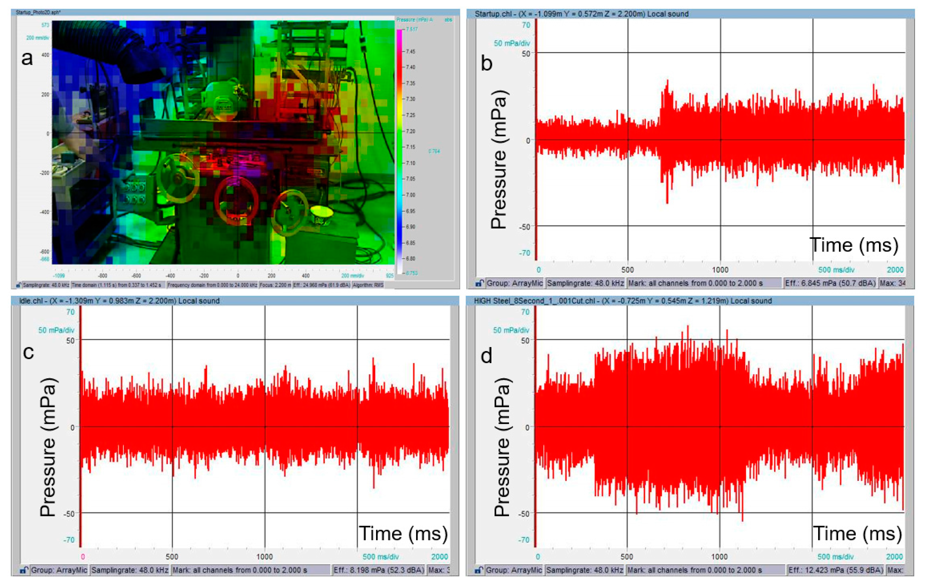
Figure 3a provides the 2D image of the machine with the noise intensity map. Figure 3b–d shows the noise as a function of time during startup, idle speed, and under load conditions. It can be seen that as the machine gets started, the noise pressure increased to an upper level and then decreased to a value during the idle condition. This is due to the jerking of starting from zero speed to a set speed. Once it reached the steady-state region the pressure decreased to the idle level. It can also be noted that the mean pressure is more than zero due to the constant background noise. Once the machine gets to an idle region the pressure value is constant (Figure 3c). During the loading condition the grinder will be in contact with the work-piece and force will be required to grind the work-piece. Thus the noise pressure increased. This increase will depend on the rpm of the grinder and feed of the stage. It is hypothesized that a lower rpm and a higher feed will increase the noise pressure and vice-versa, and lower noise pressure means the tool will last longer.
4.2. Surface Grinder
The results shown below are for a surface grinder. Figure 4a provides the 2D image for noise intensity. As compared to the bench grinder, the surface grinder has three variables for operation i.e., (i) rpm of grinder disc; (ii) depth of cut; and, (iii) feed of cut. During the startup condition the rpm of the grinder starts from 0 to the set rpm. It can be seen that due to a high rpm i.e., 2800 the grinder reached a saturation pressure faster than the bench grinder (Figure 4b). Furthermore, in the idle condition the pressure remained constant (Figure 4c). Depending on the feed of the grinder the machining time can be observed from Figure 4d. It can be observed that the cutting started at 300 ms and one feed finished at 1200 ms, i.e., total machining time was 900 ms (0.9 s). From this sample the distance of machining can be calculated for the complex part. During the grinding the noise pressure increased from the idle condition.
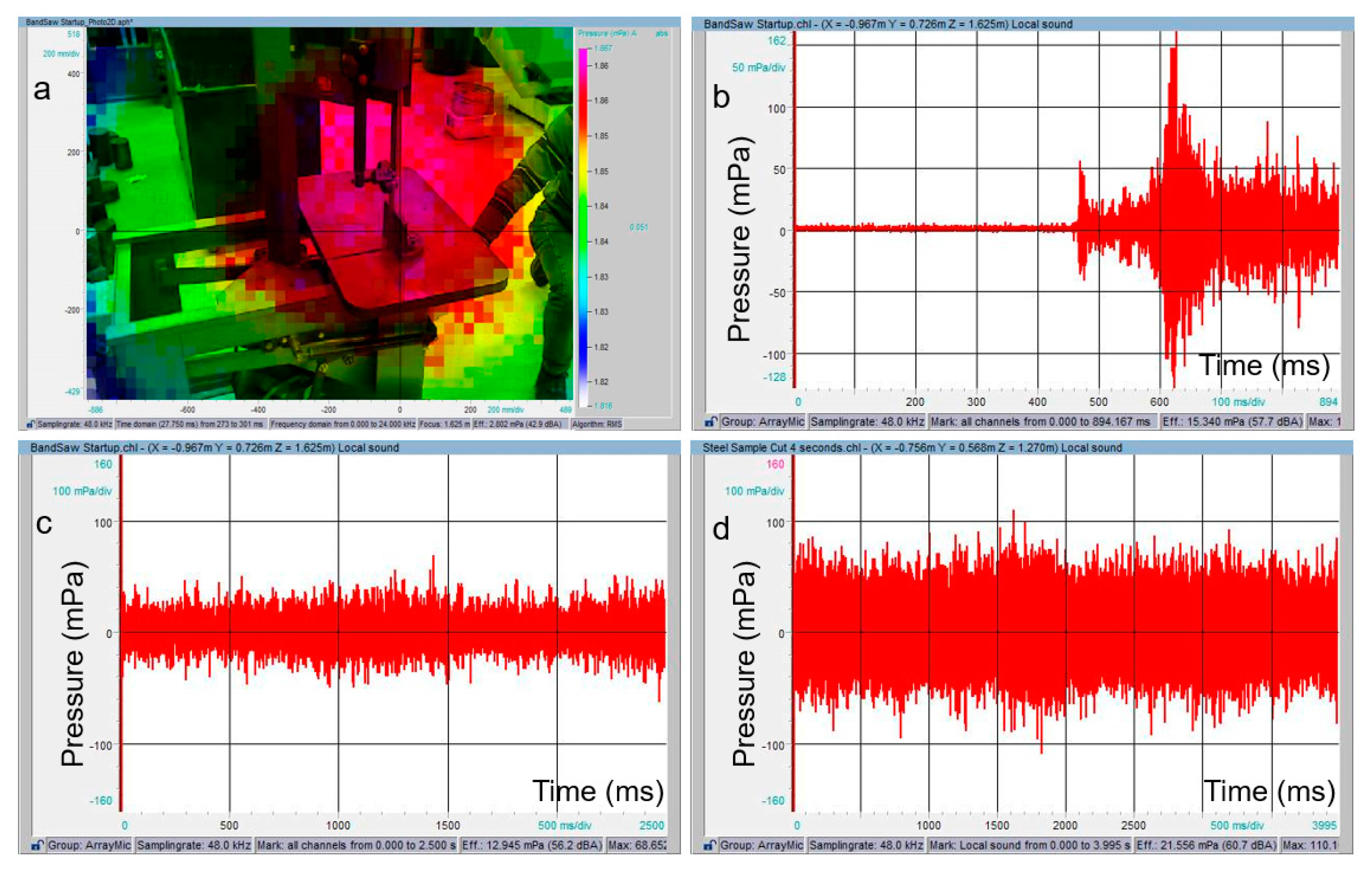
4.3. Vertical Band Saw
Similar to the previous results, the 2D image with noise intensity can be observed for the vertical band saw (Figure 5a). Here, the variables are the motor rpm and the feed of the material to the saw. During startup the motor jerked due to friction contact and settled to the idle speed (Figure 5b). Figure 5c provides the idle running noise pressure. When the blade started cutting the material the noise level increased (Figure 5d). It is hypothesized that this noise pressure can be reduced by reducing the feed of the work-piece for cutting and thus increasing the tool life.
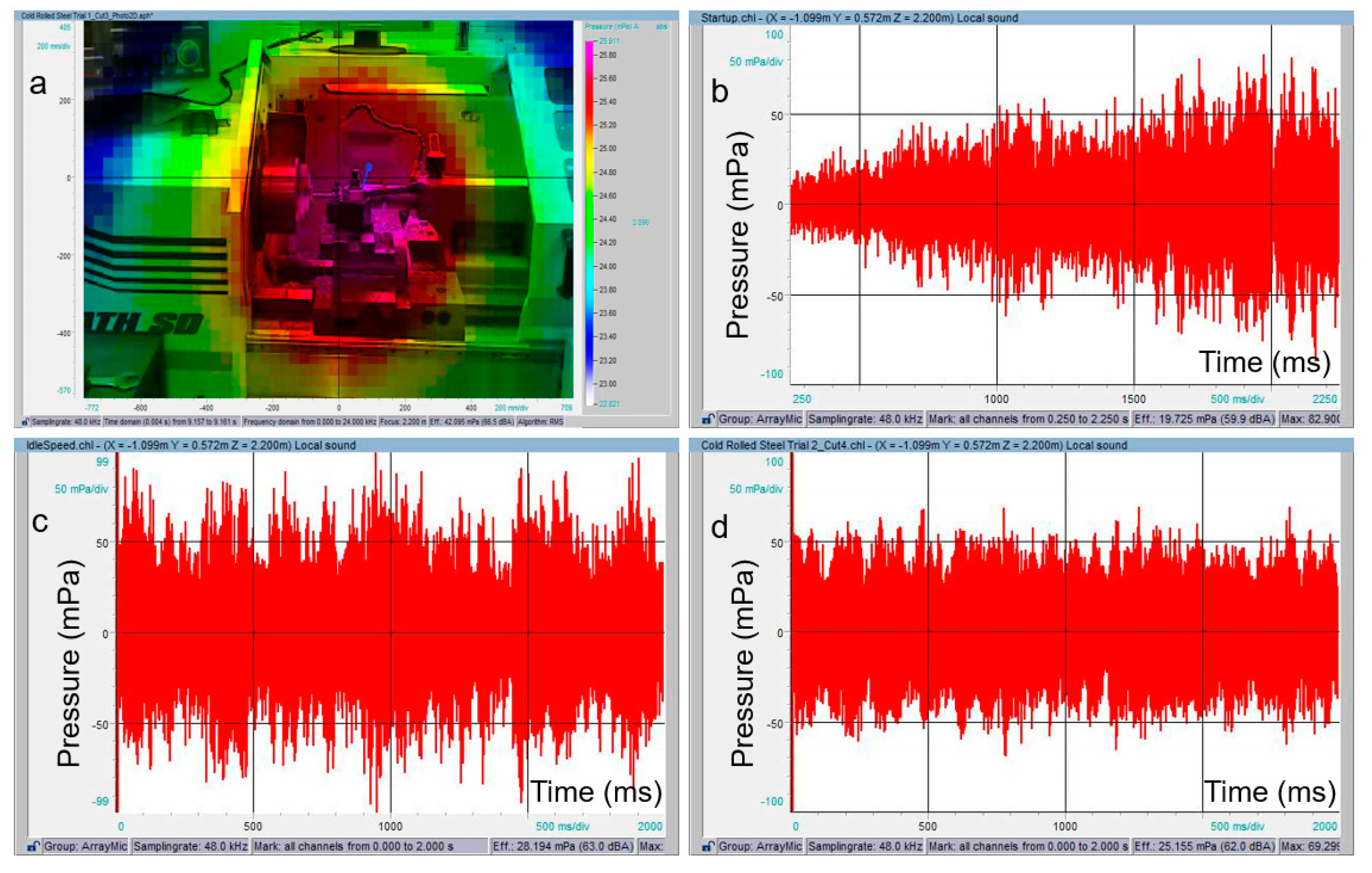
4.4. Lathe Machine
The 2D image with noise intensity is provided in Figure 6a. It can be seen that the lathe machine needs a longer amount of time before it gets to idle (Figure 6b). This is again dependent on the rpm of the chuck. As can be seen in Figure 6a, that the work-piece bar is already in the chuck. Due to the longer length of the shaft, a small eccentricity can provide the large deflection, and thus vibration and noise. The eccentricity of the material can also be determined from the noise emission. As shown in Figure 6c, the continuous peaks and valleys may be due to the eccentric mounting of a bar in the chuck. Due to this, the noise pressure was higher. However as soon as the cutting tool was in contact with the work-piece, the eccentricity may have been corrected and thus vibration and noise were reduced.
4.5. Vertical Milling Machine
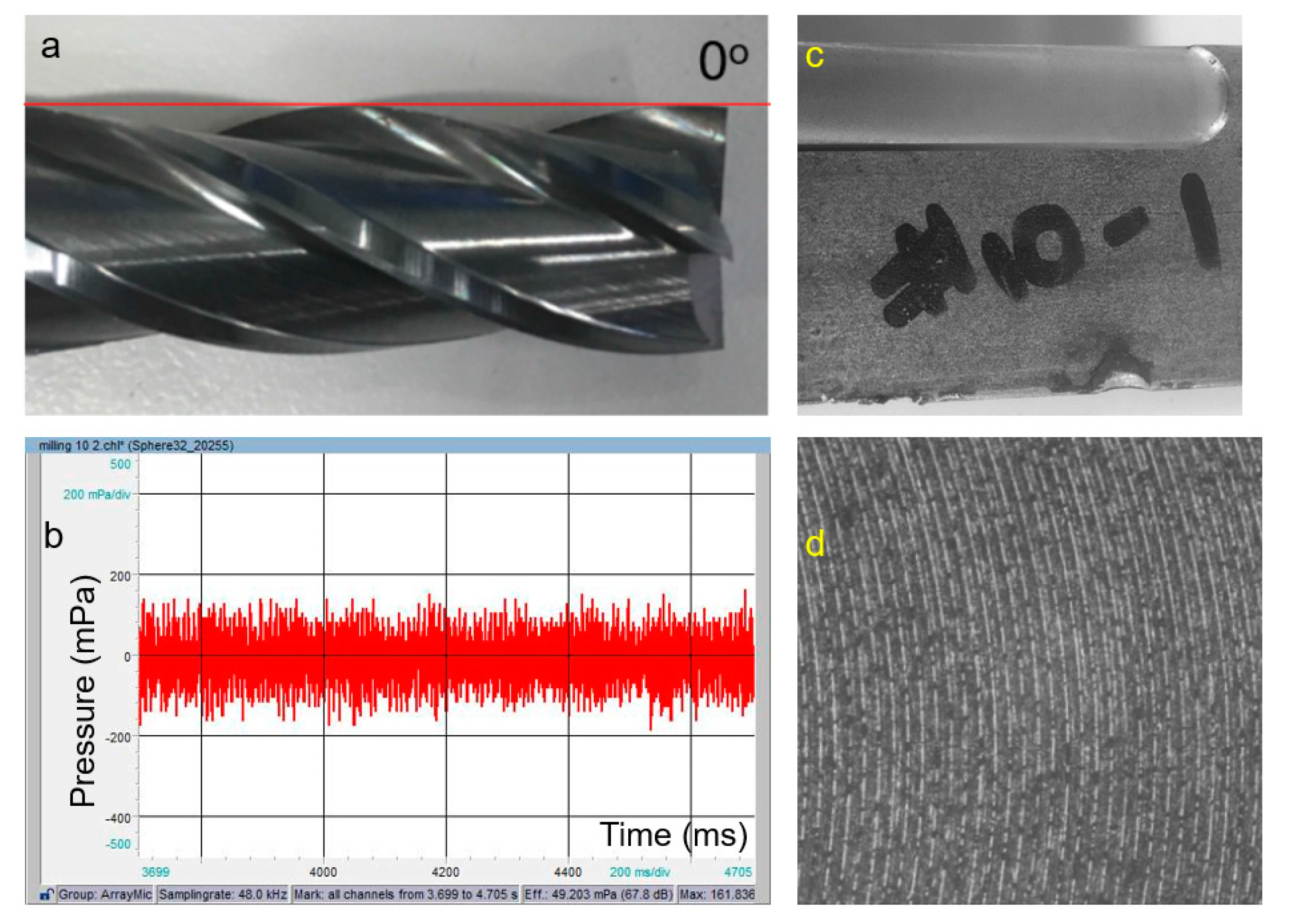
In this section the results of the vertical milling machine are discussed. The 2D image with noise intensity is shown in Figure 7a. During startup the tool picks up the speed very quickly due to having a much smaller diameter as compared to the bench or surface grinder. The higher peak noise pressure as shown in Figure 7b is due to the longer shaft length from the motor, and thus more vibration at the start. It quickly reached the machine idle condition (Figure 7c). During cutting the pressure reached a slightly higher level as compared to the idle condition. The sudden increase and decrease of noise pressure is due to when the tool bit hits the material during cutting. Depending on the number of tool bits used on a tool, the noise emission can be used to calculate the approximate rpm of the tool by counting the peaks per unit time. If the tool has four bits, than four peaks can provide one rotation of the tool. By reading the time for four peaks, the rpm can be determined. For example, Figure 7d provides approximately 10 dominant peaks in 200 ms (between 4200 to 4400 ms) in Region A. The tool has four bits (Figure 8a). Therefore, 10/4 gives 2.5 rotations of the tool in 200 ms, and thus 2.5 × 1000/200 gives 12.5 rotation per second i.e., 750 rpm, which was the set speed for this experiment. Note that the additional peaks in the noise emission data are due to background noise during the machining process.
Table 3 provides the effective sound pressure in mPa for each test machine for startup, idle, and load conditions. It can be seen that the idle speed effective sound pressure suddenly increased at load condition in the bench grinder, surface grinder, and vertical band saw. This is due to the tool contacting the work-piece. During cutting the noise level increased as compared to the idle condition. However, in both the lathe and vertical milling machines, the idle and load sound pressure values are similar. This is the result of the eccentricity in the work-piece within the chuck (lathe machine) and the eccentricity of the tool holder in the milling machine producing the noise, which is compensated during the cutting process. It is hypothesized that this may be due to the contact between the tool and work-piece, which stabilizes the process and produces less noise.
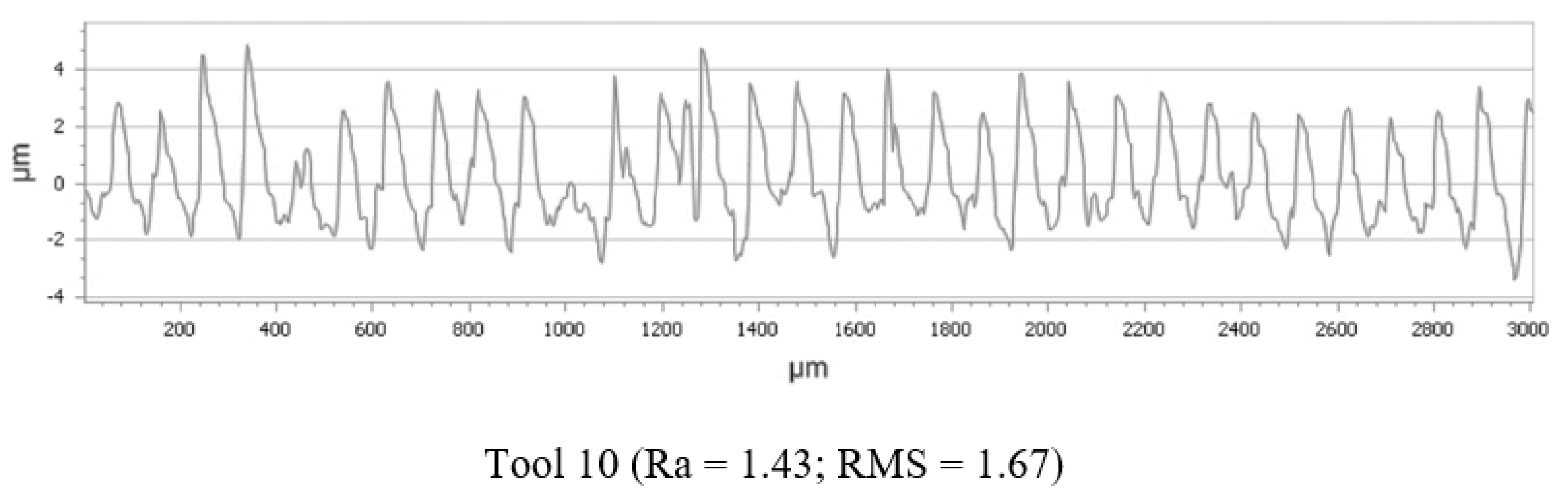
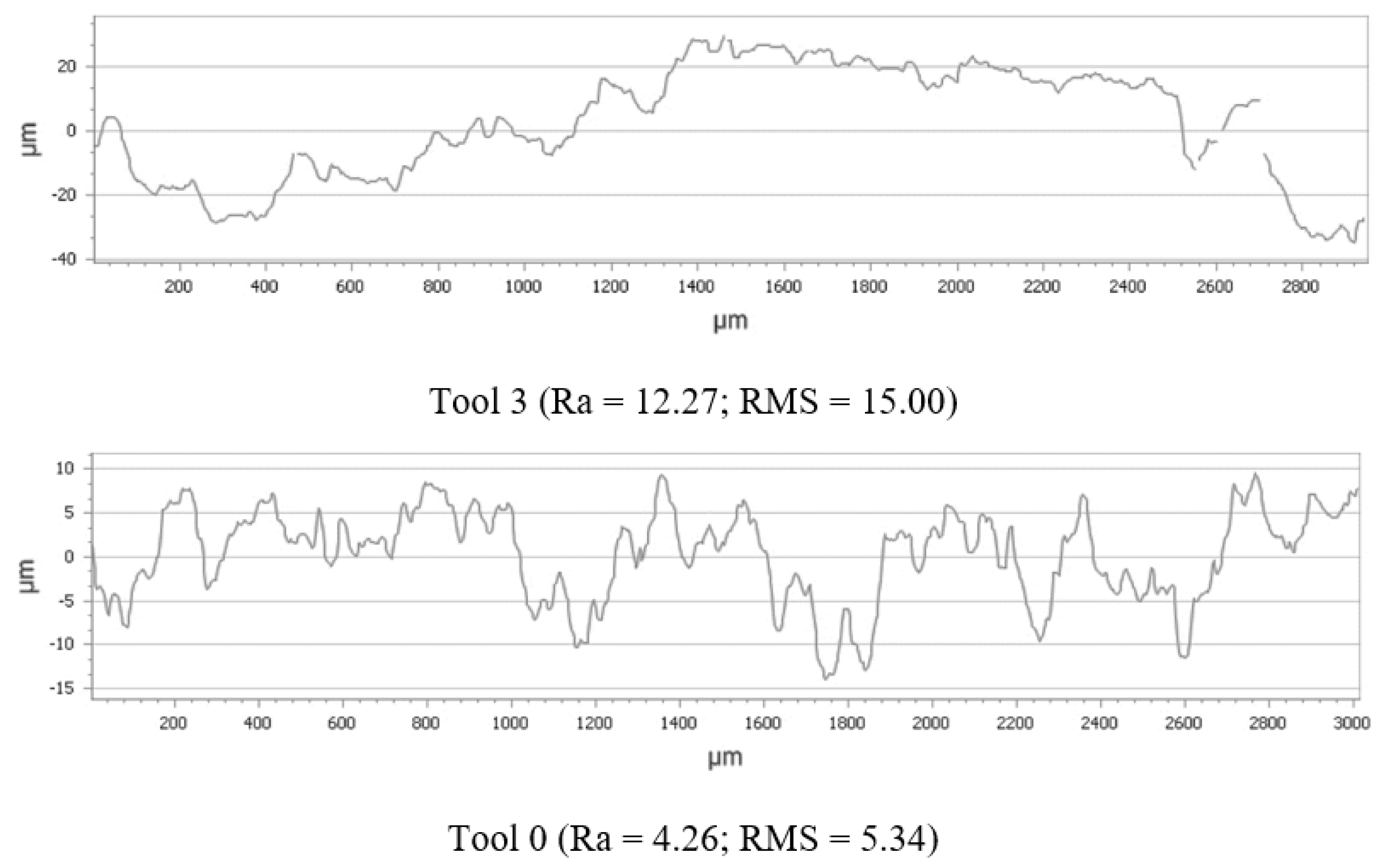
Furthermore, two more experiments were performed on the vertical milling machine with Tool 3 and Tool 0. Again, the Tool 10 name was given to a new tool and Tool 0 for the fully worn tool. It can be observed that the Tool 10 has no wear and is perfectly aligned with the red line (Figure 8a). However Tool 3 shows little wear with an angle of 5°, and Tool 0 has significant wear, with an angle of 35° (Figure 9a and Figure 10a). The effective noise pressure level during load for Tool 10 was 49.2 mPa, but it increased to 67.71 mPa for Tool 3 and saturated for Tool 0 at 68.77 mPa, as detailed in Table 4. Since the noise level for Tools 3 and 0 were very similar, this indicates that the condition of Tool 3 is not fair and needs to be replaced (Figure 8b, Figure 9b and Figure 10b). The milled conditions for all of the three tools are shown in Figure 8c, Figure 9c and Figure 10c. It shows that the milling is smooth with Tool 10, but it is compromised with Tools 3 and 0 by having a rough finish and inaccurate geometry. The surface images by Zygo surface profilometer are shown in Figure 8d, Figure 9d and Figure 10d. Uniform concentric arcs are achieved with Tool 10, but more non-uniform zones are shown with Tools 3 and 0.
The surface roughness measurements are shown in Figure 11. With Tool 10, the Ra (average roughness) and RMS (root mean square) values for surface roughness are much smaller than with Tools 3 and 0. The surface roughness value for Tool 0 is lower than Tool 3, since Tool 0 was not cutting the desired width due to the high wear angle. From Table 4, Tool 10 provides lower sound pressure as compared to Tools 3 and 0, where the noise levels were similar. The Tool 3 condition does provide the desired geometry but the surface quality is compromised. With continuous usage of the tool, it will reach the Tool 0 condition where the sound pressure saturates, but would not provide the desired geometry. Thus, tool replacement should occur no later than at the Tool 3 condition. It can be concluded that with a set amount of parameters, the point where the effective sound pressure saturates provides the indication of tool replacement.
5. Conclusions
In this paper, acoustic emission was studied for a bench grinder, surface grinder, vertical band saw, lathe machine, and vertical milling machine. These machines were selected since they use different tools to cut/machine the work-piece. Each test machine specification was studied and applied to prove the concept. To understand the noise emissions, the test machines were set to certain conditions and data was captured for startup, idle speed, and machining conditions. After analysis it was concluded that:
- (a)
- Running parameters like the type of tool, rpm, depth and feed of cut are sensitive to the noise pressure.
- (b)
- At machine startup, the noise emission provides the time to get to the idle state. Some of the machines instantly get to the idle state depending on the running rpm, but it also depends on the tool diameter and length of the tool from the motor support. For example, the bench grinder used a bigger disc than the surface grinder and took a longer time to get to the idle state. Similarly, the vertical milling machine has a long tool shaft and provides more vibration than the grinder machine.
- (c)
- During the idle condition the machine produced constant noise pressure.
- (d)
- For loading conditions, the noise pressure depends on the parameters like rpm, depth, and feed of cut. It is hypothesized that the machine will produce less noise with a higher rpm and lower feed and depth of cut.
- (e)
- With noise pressure data and knowing the tool i.e., how many bits in the tool or how many tooth in the saw, the rpm can be calculated. It is hypothesized that in a similar way the depth and feed of cut can also be determined.
- (f)
- With a set amount of parameters, the point where the effective sound pressure saturates is the time when the tool change would be required.
- (g)
- Knowledge of noise pressure can help in determining the variables which increase the tool health and life.
The above general conclusions are provided in this paper, however future work will investigate time-frequency analysis techniques, such as short-time fourier transform (STFT), and continuous wavelet transform (CWT). The spectral content of the noise emissions will be investigated to determine the complete correlation to the operating characteristics of machines during various machining processes. This would include the variation of parameters like rpm, depth of cut, feed of cut, and tool condition. Additionally, algorithms will be investigated to accurately predict the tool replacement in real-time while performing milling and various other machining operations.
Acknowledgments
This research work was supported in part by a NoiseImage software grant from GFAI Tech. The authors would also like to greatly acknowledge the support from Penn State Erie—The Behrend College for undergraduate research funding. Special thanks go to Glenn Craig for technical support during experiments.
Conflicts of Interest
The authors declare no conflict of interest.
References
- Aramesh, M.; Shaban, Y.; Yacout, S.; Attia, M.H.; Kishawy, H.A.; Balazinski, M. Survival life analysis applied to tool life estimation with variable cutting conditions when machining titanium metal matrix composites (Ti-MMCs). Mach. Sci. Technol. 2016, 20, 132–147. [Google Scholar] [CrossRef]
- Lopes Da Silva, R.H.; Bacci Da Silva, M.; Hassui, A. A probabilistic neural network applied in monitoring tool wear in the end milling operation via acoustic emission and cutting power signals. Mach. Sci. Technol. 2016, 20, 386–405. [Google Scholar] [CrossRef]
- Bhuiyan, M.S.H.; Choudhury, I.A. Investigation of tool wear and surface finish by analyzing vibration signals in turning ASSAB-705 steel. Mach. Sci. Technol. 2015, 19, 236–261. [Google Scholar] [CrossRef]
- Sanjay, C.; Neema, M.L.; Chin, C.W. Modeling of tool wear in drilling by statistical analysis and artificial neural network. J. Mater. Process. Technol. 2005, 170, 494–500. [Google Scholar] [CrossRef]
- Nouri, M.; Fussell, B.K.; Ziniti, B.L.; Linder, E. Real-time tool wear monitoring in milling using a cutting condition independent method. Int. J. Mach. Tools Manuf. 2015, 89, 1–13. [Google Scholar] [CrossRef]
- Ghosh, N.; Ravi, Y.B.; Patra, A.; Mukhopadhyay, S.; Paul, S.; Mohanty, A.R.; Chattopadhyay, A.B. Estimation of tool wear during CNC milling using neural network-based sensor fusion. Mech. Syst. Signal Process. 2007, 21, 466–479. [Google Scholar] [CrossRef]
- Patra, K.; Pal, S.K.; Bhattacharyya, K. Artificial neural network based prediction of drill flank wear from motor current signals. Appl. Soft Comput. J. 2007, 7, 929–935. [Google Scholar] [CrossRef]
- Aliustaoglu, C.; Ertunc, H.M.; Ocak, H. Tool wear condition monitoring using a sensor fusion model based on fuzzy inference system. Mech. Syst. Signal. Process. 2009, 23, 539–546. [Google Scholar] [CrossRef]
- Dimla, D.E. Sensor signals for tool-wear monitoring in metal cutting operations—A review of methods. Int. J. Mach. Tools Manuf. 2000, 40, 1073–1098. [Google Scholar] [CrossRef]
- Trent, E.M.; Wright, P.K. Metal Cutting, 4th ed.; Butterworth-Heinemann: Boston, MA, USA, 2000. [Google Scholar]
- Carvalho, S.R.; Lima e Silva, S.M.M.; Machado, A.R.; Guimarães, G. Temperature determination at the chip–tool interface using an inverse thermal model considering the tool and tool holder. J. Mater. Process. Technol. 2006, 179, 97–104. [Google Scholar] [CrossRef]
- Majumdar, P.; Jayaramachandran, R.; Ganesan, S. Finite element analysis of temperature rise in metal cutting process. Appl. Therm. Eng. 2005, 25, 2152–2168. [Google Scholar] [CrossRef]
- Shih, A.J. Finite element analysis of orthogonal metal cutting mechanics. Int. J. Mach. Tools Manuf. 1996, 36, 255–273. [Google Scholar] [CrossRef]
- Tay, A.A.O. A review of methods of calculating machining temperature. J. Mater. Process. Technol. 1993, 36, 225–257. [Google Scholar] [CrossRef]
- Smithey, D.W.; Kapoor, S.G.; DeVor, R.E. A new mechanistic model for predicting worn tool cutting forces. Machining Science and Technology. Mach. Sci. Technol. 2001, 5, 23–42. [Google Scholar] [CrossRef]
- Wang, C.; Cheng, K.; Nelson, N.; Sawangsri, W.; Rakowski, R. Cutting force-based analysis and correlative observations on the tool wear in diamond turning of single crystal silicon. J. Eng. Manuf. 2014, 229, 1–7. [Google Scholar] [CrossRef]
- Alonso, F.J.; Salgado, D.R. Analysis of the structure of vibration signals for tool wear detection. Mech. Syst. Signal Process. 2008, 22, 735–748. [Google Scholar] [CrossRef]
- Dimla, D.E. The impact of cutting conditions on cutting forces and vibration signals in turning with plane face geometry inserts. J. Mater. Process. Technol. 2004, 155–156, 1708–1715. [Google Scholar] [CrossRef]
- Dimla, D.E.; Lister, P.M. On-line metal cutting tool condition monitoring I: Force and vibration analyses. Int. J. Mach. Tools Manuf. 2000, 40, 739–768. [Google Scholar] [CrossRef]
- Ghani, A.K.; Choudhury, I.A.; Husni. Study of tool life, surface roughness and vibration in machining nodular cast iron with ceramic tool. J. Mater. Process. Technol. 2002, 37, 11–22. [Google Scholar] [CrossRef]
- Altintas, Y.; Lee, P. Prediction of ball-end milling forces from orthogonal cutting data. Int. J. Mach. Tools Manuf. 1996, 36, 1059–1072. [Google Scholar]
- Jemielniak, K.; Arrazola, P.J. Application of AE and cutting force signals in tool condition monitoring in micro-milling. CIRP J. Manuf. Sci. Technol. 2008, 1, 97–102. [Google Scholar] [CrossRef]
- Said, M.B.; Saï, K.; Saï, W.B. An investigation of cutting forces in machining with worn ball-end mill. J. Mater. Process. Technol. 2009, 29, 3198–3217. [Google Scholar] [CrossRef]
- Rangwala, S.; Dornfeld, D. A study of acoustic emission generated during orthogonal metal cutting—1: energy analysis. Int. J. Mech. Sci. 1991, 33, 471–487. [Google Scholar] [CrossRef]
- Dornfeld, D.A.; Kannatey-Asibu, E. Acoustic emission during orthogonal metal cutting. Int. J. Mech. Sci. 1980, 22, 285–296. [Google Scholar] [CrossRef]
- Kannatey-Asibu, E.; Dornfeld, D.A. A study of tool wear using statistical analysis of metal cutting acoustic emission. Wear 1982, 76, 247–261. [Google Scholar] [CrossRef]
- Kannatey-Asibu, E.; Emel, E. Linear discriminant function analysis of acoustic emission signals for cutting tool monitoring. Mech. Syst. Signal Process. 1987, 1, 333–347. [Google Scholar] [CrossRef]
- Farrelly, F.A.; Petri, A.; Pitolli, L. Statistical properties of acoustic emission signals from metal cutting processes. J. Acoust. Soc. Am. 2004, 116, 981–986. [Google Scholar] [CrossRef]
- Teti, R.; Jamielniak, K.; O’Donnell, G.; Dornfield, D. Advanced monitoring of machining operations. CIRP Ann.—Manuf. Technol. 2010, 59, 171–739. [Google Scholar] [CrossRef]
- Baccar, D.; Soffker, D. Wear detection by means of wavelet-based acoustic emission analysis. Mech. Syst. Signal Process. 2015, 60–61, 198–207. [Google Scholar] [CrossRef]
- Jamielniak, K.; Otman, O. Tool failure detection based on analysis of acoustic emission signals. J. Mater. Process. Technol. 1998, 76, 192–197. [Google Scholar] [CrossRef]
- Yan, D.; El-Wardany, T.; Elbestawi, M. A multi-sensor strategy for tool failure detection in milling. Int. J. Mach. Tools Manuf. 1995, 35, 383–398. [Google Scholar] [CrossRef]
- Milner, J.; Roth, J. Condition monitoring for indexable carbide end mill using acceleration data. Mach. Sci. Technol. 2010, 14, 63–80. [Google Scholar] [CrossRef]
- Nikhare, C.; Ragai, I.; Loker, D.; Sweeney, S.; Conklin, C.; Roth, J.T. Investigation of acoustic signals during W1 tool steel quenching. In Proceedings of the ASME International Manufacturing Science and Engineering Conference, Charlotte, NC, USA, 8–12 June 2015; pp. 1–9. [Google Scholar]
- Erich, N.J.; Nikhare, C.P.; Conklin, C.; Loker, D.R. Study of acoustic signals and mechanical properties dependence during cold drawn A36 steel quenching. In Proceedings of the International Deep Drawing Research Group Conference, Shanghai, China, 31 May–3 June 2015; pp. 338–346. [Google Scholar]
- Jaeckel, O. Strengths and weaknesses of calculating beam forming in the time domain. In Proceedings of the 1st Berlin Beam Forming Conference, Berlin, Germany, 21–22 November 2006; pp. 1–10. [Google Scholar]
- Romenskiy, I.; Jaeckel, O. Improvement of Source Separation for Phased Microphone Array Measurements. In Proceedings of the 2nd Berlin Beam Forming Conference, Berlin, Germany, 19–20 February 2008; pp. 1–8. [Google Scholar]
Figure 1.
Test machines for acoustic emission: (a) bench grinder; (b) surface grinder; (c) vertical band saw; (d) lathe machine; and, (e) vertical milling machine.
Figure 1.
Test machines for acoustic emission: (a) bench grinder; (b) surface grinder; (c) vertical band saw; (d) lathe machine; and, (e) vertical milling machine.
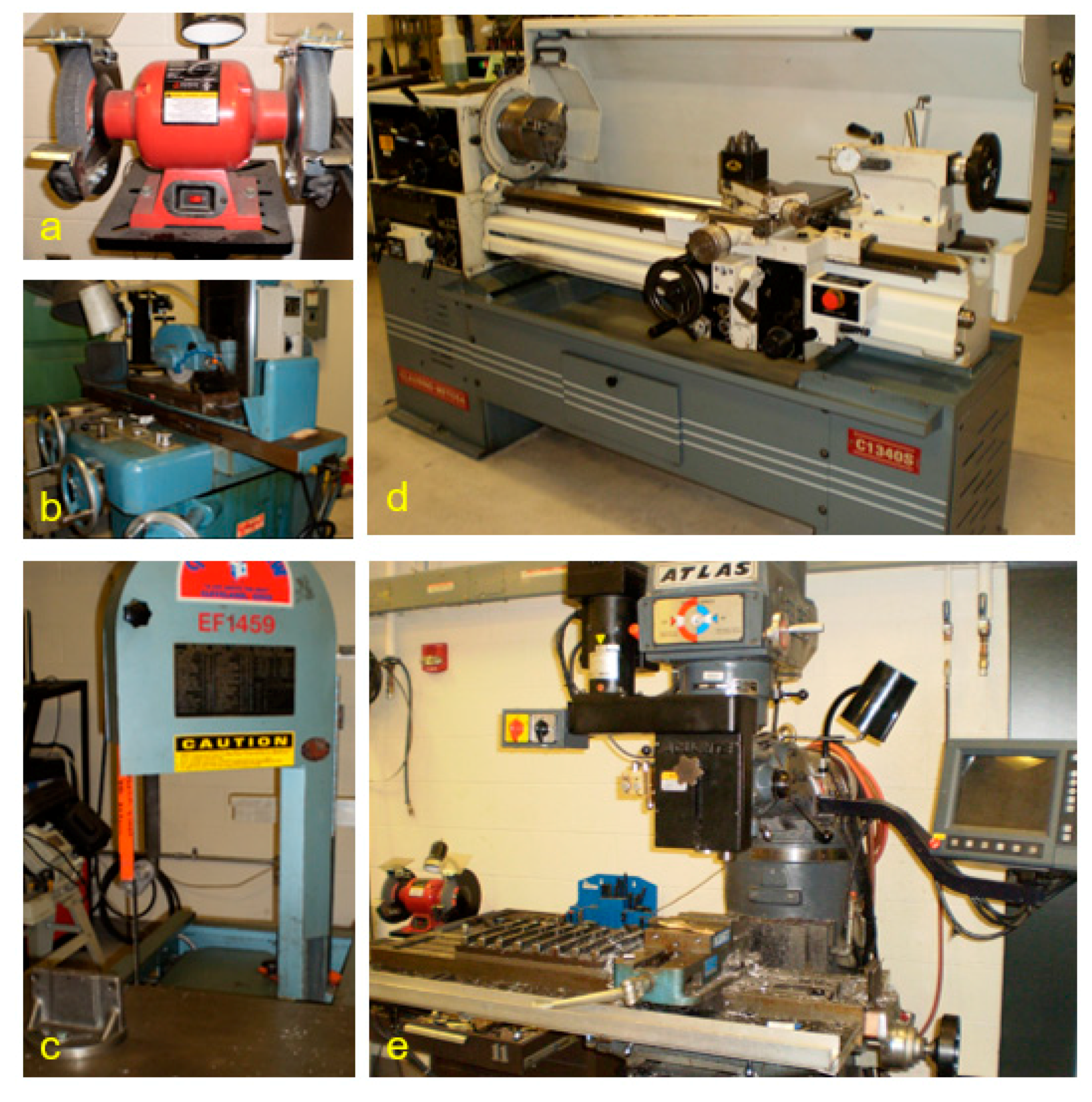
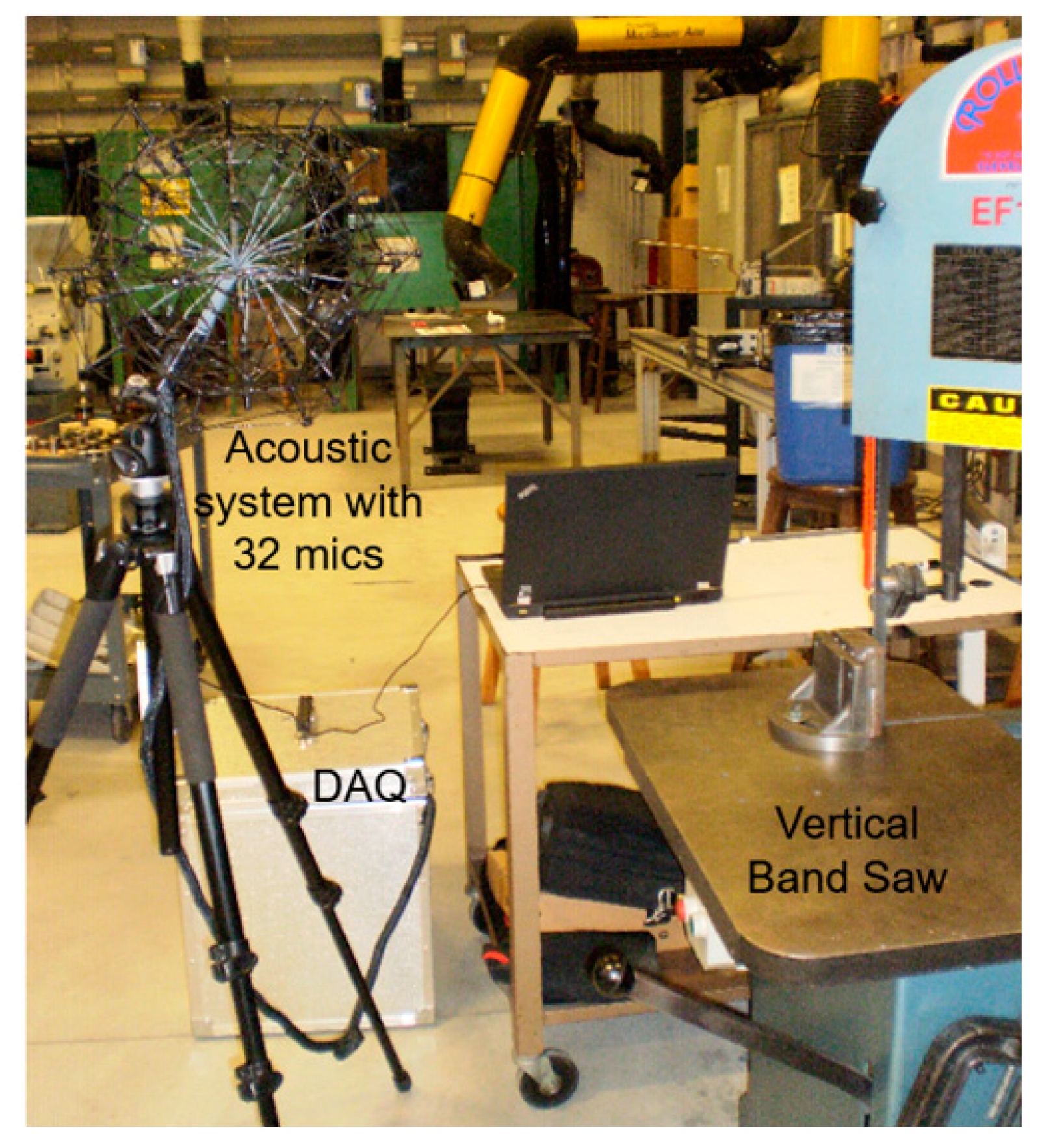
Figure 2.
Experimental set-up for acoustic emission data collection with experimental conditions.

Figure 3.
Acoustic emission for bench grinder: (a) 2D image superimposed with noise mapping intensity; (b) noise emission during startup; (c) noise emission during idle speed; and, (d) noise emission during load.
Figure 3.
Acoustic emission for bench grinder: (a) 2D image superimposed with noise mapping intensity; (b) noise emission during startup; (c) noise emission during idle speed; and, (d) noise emission during load.

Figure 4.
Acoustic emission for surface grinder: (a) 2D image superimposed with noise mapping intensity; (b) noise emission during startup; (c) noise emission during idle speed; and (d) noise emission during load.
Figure 4.
Acoustic emission for surface grinder: (a) 2D image superimposed with noise mapping intensity; (b) noise emission during startup; (c) noise emission during idle speed; and (d) noise emission during load.

Figure 5.
Acoustic emission for vertical band saw: (a) 2D image superimposed with noise mapping intensity; (b) noise emission during startup; (c) noise emission during idle speed; and (d) noise emission during load.
Figure 5.
Acoustic emission for vertical band saw: (a) 2D image superimposed with noise mapping intensity; (b) noise emission during startup; (c) noise emission during idle speed; and (d) noise emission during load.

Figure 6.
Acoustic emission for lathe machine: (a) 2D image superimposed with noise mapping intensity; (b) noise emission during startup; (c) noise emission during idle speed; and (d) noise emission during load.
Figure 6.
Acoustic emission for lathe machine: (a) 2D image superimposed with noise mapping intensity; (b) noise emission during startup; (c) noise emission during idle speed; and (d) noise emission during load.

Figure 7.
Acoustic emission for vertical milling machine (a) 2D image superimposed with noise mapping intensity; (b) noise emission during startup; (c) noise emission during idle speed; and (d) noise emission during load.
Figure 7.
Acoustic emission for vertical milling machine (a) 2D image superimposed with noise mapping intensity; (b) noise emission during startup; (c) noise emission during idle speed; and (d) noise emission during load.
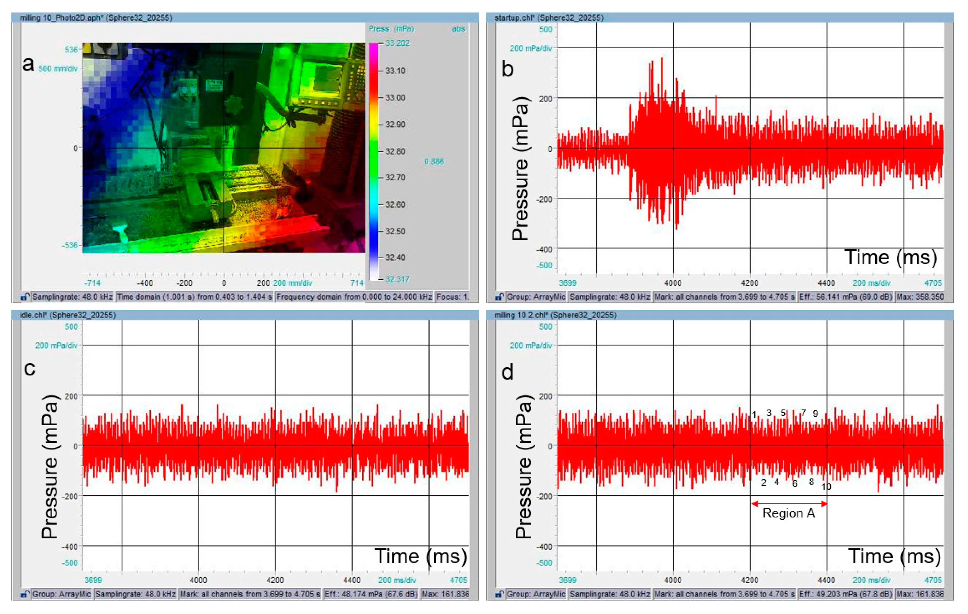
Figure 8.
Acoustic and surface measurement for Tool 10 during milling: (a) image of tool with wear condition; (b) noise emission during load (Feed = 3 in/min; depth of cut = 0.05 in and RPM = 750); (c) milled piece; and (d) image on surface roughness.
Figure 8.
Acoustic and surface measurement for Tool 10 during milling: (a) image of tool with wear condition; (b) noise emission during load (Feed = 3 in/min; depth of cut = 0.05 in and RPM = 750); (c) milled piece; and (d) image on surface roughness.

Figure 9.
Acoustic and surface measurement for Tool 3 during milling: (a) image of tool with wear condition; (b) noise emission during load (Feed = 3 in/min; depth of cut = 0.05 in and RPM = 750); (c) milled piece; and (d) image on surface roughness.
Figure 9.
Acoustic and surface measurement for Tool 3 during milling: (a) image of tool with wear condition; (b) noise emission during load (Feed = 3 in/min; depth of cut = 0.05 in and RPM = 750); (c) milled piece; and (d) image on surface roughness.
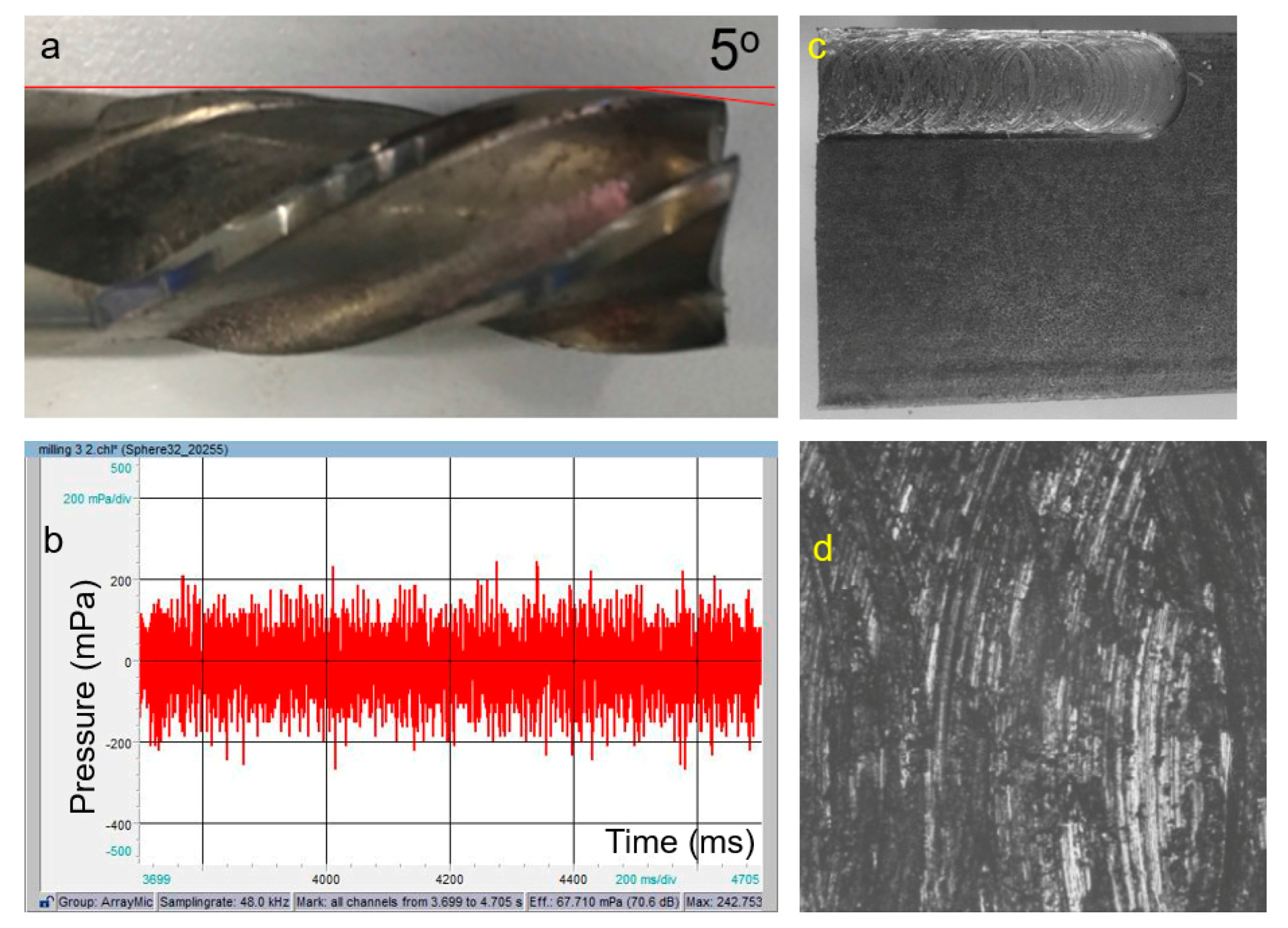
Figure 10.
Acoustic and surface measurement for Tool 0 during milling: (a) image of tool with wear condition; (b) noise emission during load (Feed = 3 in/min; depth of cut = 0.05 in and RPM = 750); (c) milled piece; and (d) image on surface roughness.
Figure 10.
Acoustic and surface measurement for Tool 0 during milling: (a) image of tool with wear condition; (b) noise emission during load (Feed = 3 in/min; depth of cut = 0.05 in and RPM = 750); (c) milled piece; and (d) image on surface roughness.
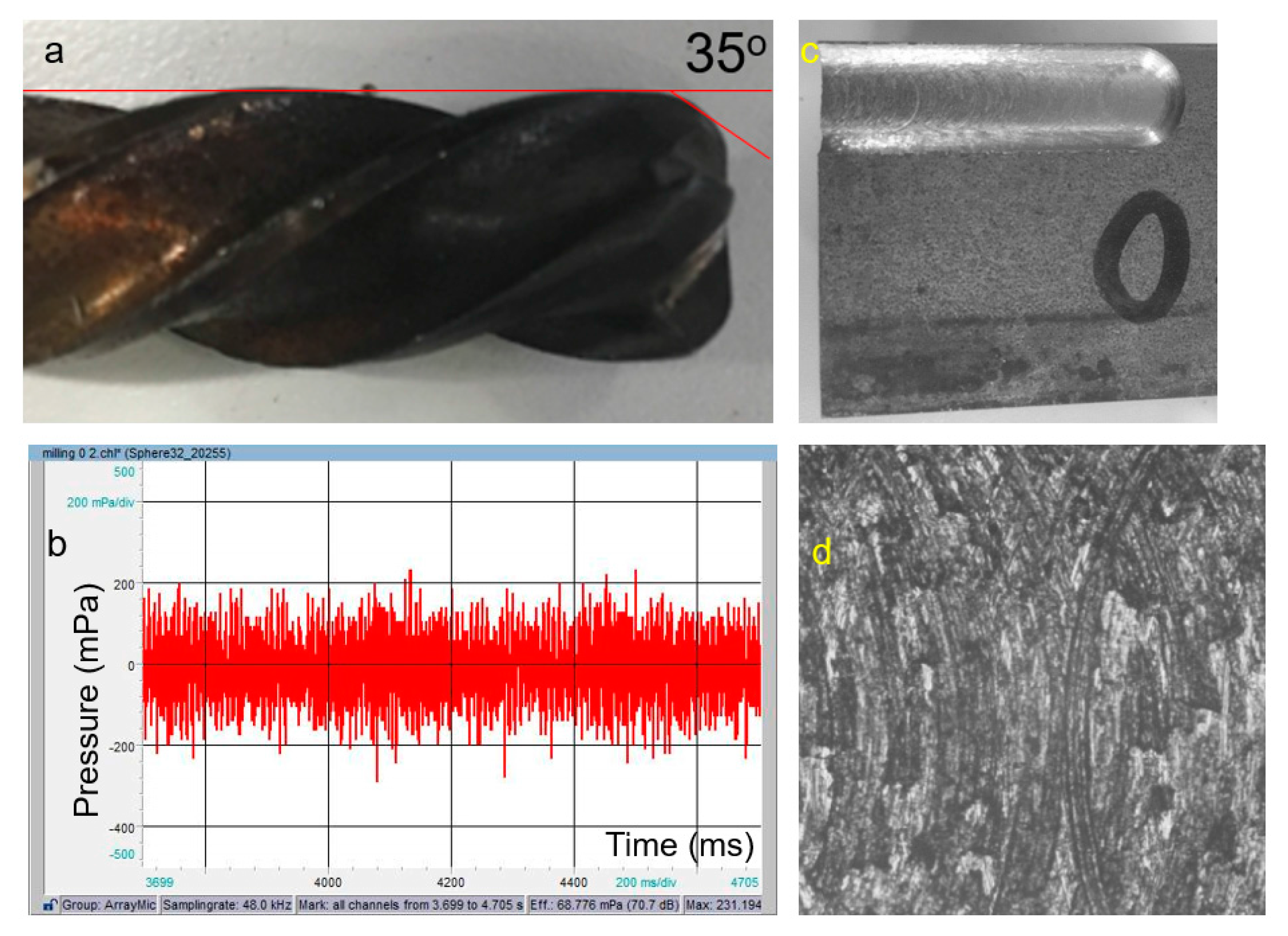
Figure 11.
Surface roughness measurement for Tool 10, 3 and 0.

Table 1.
Test machines’ specifications for acoustic emission (RPM—Revolution per minute).
| Test Machine | Power | RPM | Condition/Age | # of Motors | # of Bearings |
|---|---|---|---|---|---|
| Bench Grinder | 115v AC, 0.56 kW | 3450 | Very Good | 1 | >2 |
| Surface Grinder | 240v AC, 0.74 kW | 2800 | Good | 1 | >4 |
| Vertical Band Saw | 115v AC, 0.74 kW | 1725 | Good | 1 | >6 |
| Lathe | 240v AC, 7.45 kW | 150–2500 | Very Good | >1 | >10 |
| Vertical milling machine | 240v AC, 2.24 kW | 150–2500 | Good | >1 | >10 |
Table 2.
Conditions for experiments (Tool condition on a scale of 10–0: Tool 10 (new tool) and Tool 0 (worn tool).
Table 2.
Conditions for experiments (Tool condition on a scale of 10–0: Tool 10 (new tool) and Tool 0 (worn tool).
| Test Machine | Power | RPM | Tool Condition | Material Used |
|---|---|---|---|---|
| Bench Grinder | 115v AC, 0.56 kW | 3450 | Tool 9 | 1018 Steel |
| Surface Grinder | 240v AC, 0.74 kW | 2800 | Tool 9 | 1018 Steel |
| Vertical Band Saw | 115v AC, 0.74 kW | 1725 | Tool 9 | 1018 Steel |
| Lathe | 240v AC, 7.45 kW | 750 | Tool 9 | 1018 Steel |
| Vertical milling machine | 240v AC, 2.24 kW | 750 | Tool 10 | 1018 Steel |
Table 3.
Effective sound pressures for all 5 test machines at startup, idle and during load.
| Test Machine | Effective Sound Pressure (mPa) | ||
|---|---|---|---|
| Startup | Idle | Load | |
| Bench Grinder | 10.00 | 8.62 | 15.81 |
| Surface Grinder | 6.84 | 8.19 | 12.43 |
| Vertical Band Saw | 15.34 | 12.95 | 21.55 |
| Lathe | 19.72 | 28.19 | 25.15 |
| Vertical milling machine | 56.14 | 48.17 | 49.20 |
Table 4.
Effective sound pressure for three different milling tool condition.
| Tool Condition | Effective Sound Pressure (mPa) |
|---|---|
| Tool 10 | 49.20 |
| Tool 3 | 67.71 |
| Tool 0 | 68.77 |
© 2017 by the authors. Licensee MDPI, Basel, Switzerland. This article is an open access article distributed under the terms and conditions of the Creative Commons Attribution (CC BY) license (http://creativecommons.org/licenses/by/4.0/).
Share and Cite
MDPI and ACS Style
Nikhare, C.P.; Conklin, C.; Loker, D.R. Understanding Acoustic Emission for Different Metal Cutting Machinery and Operations. J. Manuf. Mater. Process. 2017, 1, 7. https://doi.org/10.3390/jmmp1010007
AMA Style
Nikhare CP, Conklin C, Loker DR. Understanding Acoustic Emission for Different Metal Cutting Machinery and Operations. Journal of Manufacturing and Materials Processing. 2017; 1(1):7. https://doi.org/10.3390/jmmp1010007
Chicago/Turabian StyleNikhare, Chetan P., Chris Conklin, and David R. Loker. 2017. "Understanding Acoustic Emission for Different Metal Cutting Machinery and Operations" Journal of Manufacturing and Materials Processing 1, no. 1: 7. https://doi.org/10.3390/jmmp1010007