Octree-Based Generation and Variation Analysis of Skin Model Shapes


1
Production Engineering, Royal Institute of Technology (KTH), Brinellvägen 68, 114 28 Stockholm, Sweden
2
LEAX Falun AB, Främbyvägen 30, 791 52 Falun, Sweden
*
Author to whom correspondence should be addressed.
J. Manuf. Mater. Process. 2018, 2(3), 52; https://doi.org/10.3390/jmmp2030052
Submission received: 8 July 2018
/
Revised: 1 August 2018
/
Accepted: 8 August 2018
/
Published: 12 August 2018
(This article belongs to the Special Issue Smart Manufacturing Processes in the Context of Industry 4.0)
Abstract
:The concept of Skin Model Shape has been introduced as a method for a close representation of manufactured parts using a discrete geometry representation scheme. However, discretized surfaces make irregular polyhedra, which are computationally demanding to model and process using the traditional implicit surface and boundary representation techniques. Moreover, there are still some research challenges related to the geometrical variation modelling of manufactured products; specifically, methods for geometrical data processing, the mapping of manufacturing variation sources to a geometric model, and the improvement of variation visualization techniques. To provide steps towards addressing these challenges this work uses Octree, a 3D space partitioning technique, as an aid for geometrical data processing, variation visualization, variation modelling and propagation, and tolerance analysis. Further, Skin Model Shapes are generated either by manufacturing a simulation using a non-ideal toolpath on solid models of Skin Model Shapes that are assembled to non-ideal fixtures or from measurement data. Octrees are then used in a variation envelope extraction from the simulated or measurement data, which becomes a basis for further simulation and tolerance analysis. To illustrate the method, an industrial two-stage truck component manufacturing line was studied. Simulation results show that the predicted Skin Model Shapes closely match to the measurement data from the manufacturing line, which could also be used to map to manufacturing error sources. This approach contributes towards the application of Octrees in many Skin Model Shape related operations and processes.
1. Introduction
The geometrical characteristics of all manufactured parts are inherently imperfect and disparate due to manufacturing process factors. These characteristics manifest in the form of geometric deviations from nominal models. Computer Aided Tolerancing (CAT) tools deploy classical methods, such as Vectorial Tolerancing [1], Small Displacement Torsor [2], and Tolerance-maps [3] to represent these deviations and perform tolerance analysis. These methods focus only on translational and rotational effects of variation, ignoring form effects, and not conforming to the Geometrical Product Specification (GPS) standard [4]. To overcome the shortcomings of the classical methods, the concept of Skin Model, and its extension Skin Model Shape, has been proposed to include form errors and conform to the standards [4]. Skin Model Shape (here after SMS) is created from implicit surfaces by discretized surface meshes or from readings of tactile and optical measurement tools in the form of point clouds. To obtain a high accuracy of an SMS in representation of a part, a dense mesh or point cloud is required.
However, the computational cost scales up with mesh density and the number of sampled points per part. The meshes and the reconstructed point clouds form irregular polyhedra, whose representation, operation, and manipulation, based on implicit surfaces and boundary representation techniques, is computationally slow and memory intensive [5,6,7]. Since the prime aim of utilizing SMSs is to get a detailed digital representation of parts, computational efficacy of SMS modelling and operations is crucial. As an alternative, an approach based on a 3D space partitioning technique, using Octrees, has been proven to significantly improve computation time and memory in manipulation and processing of irregular polyhedra [8,9,10]. This work utilizes the computational efficacy of Octrees, in one hand, and their capability to localize regions of form errors, in the other hand, in the generation and variation analysis of SMSs.
Moreover, despite many contributions in SMS generation methods and associated operations, there are still some challenges that need to be addressed; specifically, the mapping of manufacturing variation sources to geometric models, the development of geometrical data processing methods applicable in different stages of variation modelling, and the improvement of variation visualization techniques [11]. To address these challenges, in the context of manufacturing, process simulation, variation analysis and tolerance analysis, focused studies are some of the key steps. This would require statistical study of the manufacturing processes and shapes; Statistical Shape Analysis is an ideal tool for the purpose.
Depending on the availability of product and process information, two stages have been proposed for SMS generation and variation analysis: prediction and observation stages [4]. In this paper, for sake of completeness, we have added a tolerance analysis as a final stage of the process. In the prediction stage, SMSs are generated by a CAM simulation by inducing errors to a virtual part at each setup. In the observation stage the manufactured part prototypes are measured, the variation envelope extracted, and the surfaces are reconstructed. Both stages utilize Statistical Shapes Analysis principles with the help of Octree. In the tolerance analysis, minimum and maximum deviations from specific regions, that are used to make a variation envelope, become a basis for the tolerance analysis. In short, the novelty of this work is in the methodology of predicting an SMS of a product produced in the multistage machining process. The paper contribution includes, but is not limited to, the following:
- Recognition of Octree as a means to localize and capture a range of form errors, and as an aid for geometrical data processing, variation visualization and surface reconstruction.
- Mapping of manufacturing errors to SMS in multistage production settings and the generation of an associated variation propagation model.
The remainder of this paper is organized as follows. In Section 2, related works are reviewed. In Section 3, the proposed methodology is presented. In Section 4, the theoretical foundation of Statistical Shapes Analysis using Octrees is introduced. In Section 5, Section 6, Section 7 and Section 8, the application of the methodology in prediction, observation and tolerance analysis stages, and associated illustration case is presented. In Section 9, the results are discussed. In the last section, the conclusion and future work is presented.
2. Related Works
The current CAT tools have been criticized for overlooking form errors and non-conformance to ISO and ASME standards; the concept of SMS has been proposed to overcome these weaknesses (e.g., [4]). Thus far, the SMS concept has been applied in the tolerance analysis of non-ideal spur gears with non-ideal surfaces [12], tolerance analysis by scaling nominal mesh models [13], the mapping of non-ideal surfaces to the GD&T scheme [14], surface reconstruction from data points using NURBS followed by a Boolean operation [15], and connecting the nominal model points with data points through a spring analogy approach [16]. Despite these efforts, there is a need for more research work on easier geometrical variation modelling approaches, interoperability between computer aided tools, approaches for geometrical data processing, geometrical deviation visualization, and the mapping of variation sources to virtual products [11].
To address some of the challenges where a Statistical Shape Analysis can be utilized. One of the early research works related to Statistical Shape Analysis was made with the help of Design of Experiments to study the effect of change of the depth of cut and the cutting speed on the circularity of a physical part [17]. More recently, a Statistical Shape Analysis for a 2D surface on a regularly partitioned surface has been presented in [18]. The approach is based on a Point Distribution Model with kernel Density Estimates (PDM-KDE) [19], which is a valuable technique in extracting the systemic and random error parameters of data points and in generating a statistical shape model. However, the PDM-KDE based approach is not computationally efficient for high density data points [19].
Moreover, most of manufactured parts pass through multiple stages, during which the manufacturing error is propagated at each stage. Current error propagation modelling approaches based on mathematical formulations, such as the Differential Motion Vectors, Equivalent Fixture Error, and Kinematic Analysis, focus only on the translational and rotational aspects of variation propagation in multistage manufacturing [20]. As an alternative to the mathematical approximation, geometric characteristics can be obtained via manufacturing simulation and rendering. Towards this effort, manufacturing simulation has been utilized to study the effects of deformed dies on the surface topology of sheet metals [21], the effects of a rotary-axis [22], and machine tool motion errors [23] on the geometric characteristics of machined surfaces. These approaches basically deploy similar techniques that include inducing manufacturing errors during simulation. The approaches are useful for mapping error sources to the geometric characteristics of the parts. However, these efforts focus on a prediction of the geometric characteristics of parts produced from a single stage production line.
Octrees have the potential to address some of the challenges stated above. Octrees have been applied in slicing models for use in additive manufacturing [24], CAM simulation [6], surface reconstruction from data points [10], variation visualization [9], segmentation of data points [25], and data point reduction [26]. Despite their versatility, Octrees have not been directly applied in the generation of SMSs and associated variation analysis.
3. Methodology
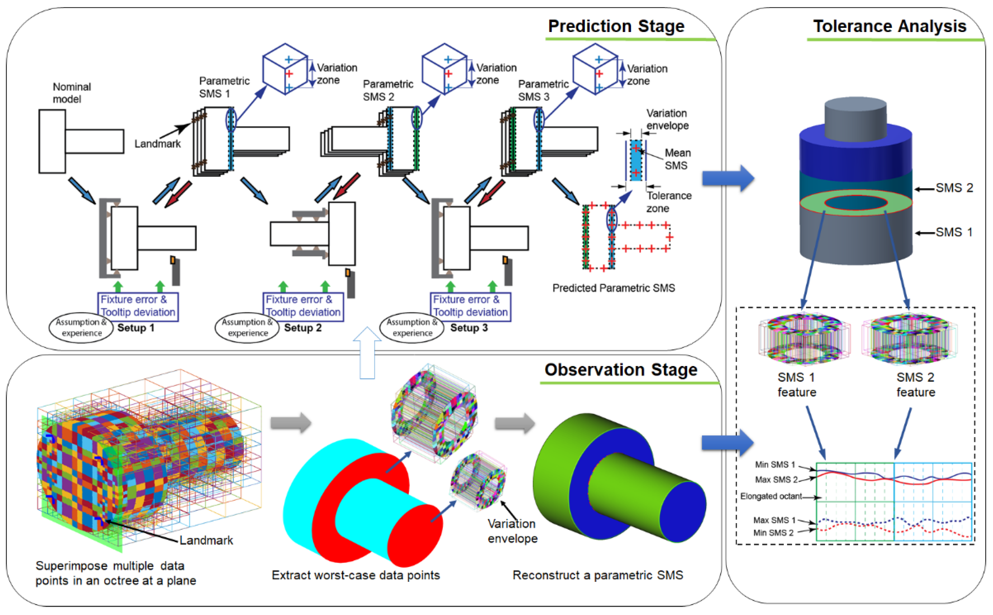
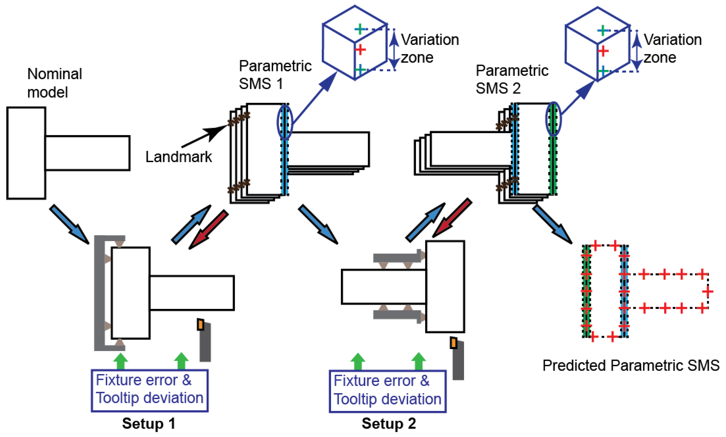
The methodology proposed in this paper extends an SMS generation and variation analysis method proposed in [4], by introducing the concept of Octrees. Specifically, the focus is on the manufacturing aspect of the method, when the manufacturing process information is available. The method is broadly divided into prediction and observation stages, both of which are followed by a variation envelope extraction, as shown in Figure 1. For the sake of completeness, tolerance analysis, the main application of SMS, is added as a stage in the methodology.
To create an Octree, a cubic bounding box that encapsulates all data points, known as a root node, is recursively subdivided into eight cubes, also referred to as Octants, until further subdivision is unnecessary. Subdivision is performed based on some termination criteria, such as extent of variation per octant [26], number of points per octant, or number of subdivisions. The number of subdivisions indicate the Octree depth and the octant of the last subdivision is referred to as the leaf octant.
In the prediction stage, two major sources of errors, fixtures and tooltip deviation, are mapped to a virtual product by inducing errors in a simulation setup. To induce those errors, pre-estimated machine capability or range of deviation of the sources of error, are used to displace virtual fixtures and machine tool parameter values to generate non-nominal toolpath. The range of the deviations of the SMS surfaces tooltip and part datum error, with a constant fixture error, are used as input factors for the Design of Experiments. The simulated responses of the experiments become predicted SMSs when random errors are added. The collection of the worst-case points per octant of the predicted SMSs are then used as inputs to the succeeding stations. Alternatively, process statistics information could be used to displace the fixture and change toolpath parameters accordingly. Moreover, it is worth mentioning that the manufacturing simulation is categorized in the prediction stage, since no training data is used, and geometric deviation is incorporated to a nominal model based on assumptions and experience.
In the observation stage, the physical parts’ data is collected from tactile and optical devices, followed by a statistical comparison of homologues regions and the surface reconstruction. To make a statistical comparison, measured data points are superimposed, and the octants are elongated in such a way that a single octant can accommodate each of the homologues points. The surface is reconstructed from the data points via the Screened Poisson Surface Reconstruction technique. The data collected in this stage can be used in predicting the SMSs of parts produced in the subsequent stations.
In a tolerance analysis, the minimum, maximum and mean points per an elongated-octant are used to perform a worst-case and statistical tolerance analysis. The mean points are displaced between minimum and maximum deviations and the stalk of the assembled SMSs is used to obtain a position deviation from the nominal assembly.
4. Statistical Shape Analysis
Statistical Shape Analysis (SSA) is a statistical technique for the comparing geometrical characteristics of shapes. In this work, we extend a previous application of SSA in manufacturing [27] and in SMS generation [18] using Octrees. The process of performing SSA follows two stages: Generalized Procrustes Algorithm, a method of comparison of shapes whose main technique is registration, and multivariate statistical methods.
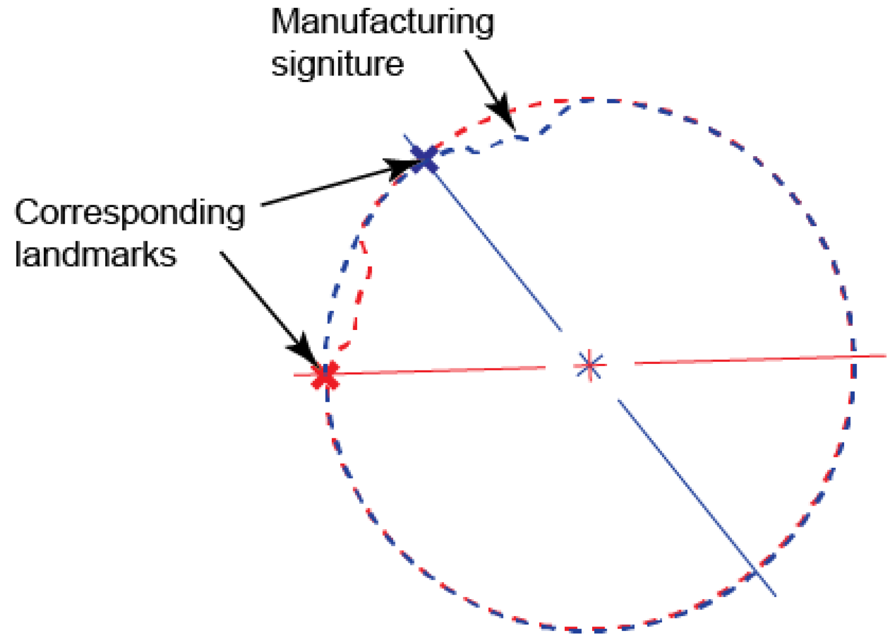
In Procrustes-based registration equal number of points, both data and reference points are required [27]. To compare multiple shapes, pre-selected reference points or regions of a shape, referred as landmarks, are registered to corresponding landmarks of another. When it comes to SMSs, there may not exist sensible corresponding points, especially in SMSs obtained from optical devices. By utilizing the same Octree for all SMSs, however, points or regions of interest can be matched, thereby making it easy to align consistent manufacturing signatures. For instance, a landmark on a turned part can end up in different rotation angles, away from their corresponding reference landmark, as is shown in Figure 2. Moreover, given the general difficulty of landmark matching in 3D space [27] and the foremost application of SMS is tolerance analysis, which is normally performed in relation to a reference datum (plane or point), landmark for registration can safely focus on a feature’s plane or points. Mathematically, the Procrustes distance (PD) of two point clouds with number of points, and , is estimated by:
In a multivariate statistical shape analysis, the effects of manufacturing processes on part shape are visualized and the effects are studied. Taking advantage of space partitioning using Octrees, the deviation of points from the nominal surface and the relationship among the points within an octant can be studied. From a manufacturing point of view, five variation related parameters are important for statistical analysis: mean, minimum (min), maximum (max), standard deviations, and process capability index at each octant. Using the first three parameters, a range of deviations within an octant can be used to create parametric SMSs, which indirectly contain manufacturing variation information.
4.1. Parametric Skin Model Shapes
Parametric modelling is one of the main techniques in CAD modelling and tolerancing. Using the parametric modelling techniques of CAT tools, the dimensions of the features are changed, and the effect of error propagation studied (e.g., [13,28]). These tools ignore form errors and assume all manufactured parts of a batch have the same geometric properties.
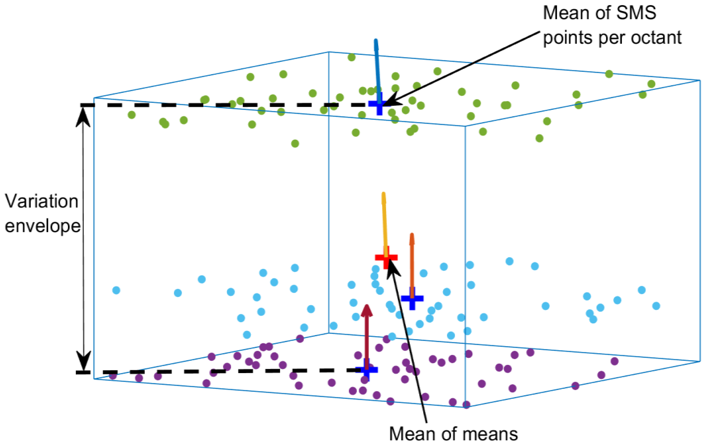
However, all manufactured parts are inherently different; hence, a single SMS cannot be an accurate representative of multiple parts. Mean shape is often used as an approximate representation of parts from the same batch (e.g., [15,18]). In addition to the mean shape, a value range per octant of superimposed SMSs is required to create a parametric SMS that encapsulates variation. Since only one shape at a time is used for the tolerance analysis and manufacturing simulation, in addition to the range of deviations, a mean shape of SMS can be incorporated into the model. Mean points can then be displaced between the min and max positions. Hence, a parametric SMS holds a mean shape and information about the deviation ranges at each octant, which makes it a better representative model. Figure 3 shows the mean point that would be used to make the mean shape, and its min and max points that make the worst-case SMS. Mathematically, for the equal number of points per octant, a set of superimposed point clouds where is the number of points per octant and the number of separate point clouds per octant, the set of all mean points , the mean of means and the worst-case tuple can be expressed as:
where is a normal vector in the normal direction to a nominal model with points that correspond to Hence contains the mean points of the two point clouds positioned at the extreme ends of an octant in the direction of .
Using the above approach, the data points per octant per SMS are reduced to a single point whose deviation is an average deviation of the points. The accuracy of the reduction is highly dependent in the number of points and variation per octant. In regions of high variation, octants are adaptively subdivided to smaller octants until the variation is kept below the predetermined level; in contrast, for low variation regions, larger octants can be used [26]. The number of reduced points to a single point has the advantage of smoothing the surfaces by canceling the random deviations.
Nevertheless, since the number of points per SMS per octant affects the mean point position, the mean points of each SMS per octant are used to compute the mean shape points. Furthermore, when a CMM is used to collect data, the octant size is modified so that all of the sample points of a specific region will lie within an octant. The number of points is reduced to the mean values of each SMS in case of optical data, but there is no need to reduce the CMM data if homologues points lie within an octant.
Moreover, to reconstruct the surfaces from the measurement data, normal vectors at each mean point need to be estimated. For a highly course partitioning where octant dimensions are significantly larger than the flatness of the surface, the third principal component, obtained by performing a Principal Component Analysis (PCA), can be used as a normal vector [18]. However, for smaller octants with at least three points, best fitting plane to points in an octant can applied. The normal vector of the plane can then be used to determine the orientation of the points at their corresponding means. The vectors are flipped or kept in the same sign as the normal vector direction of the nominal surface.
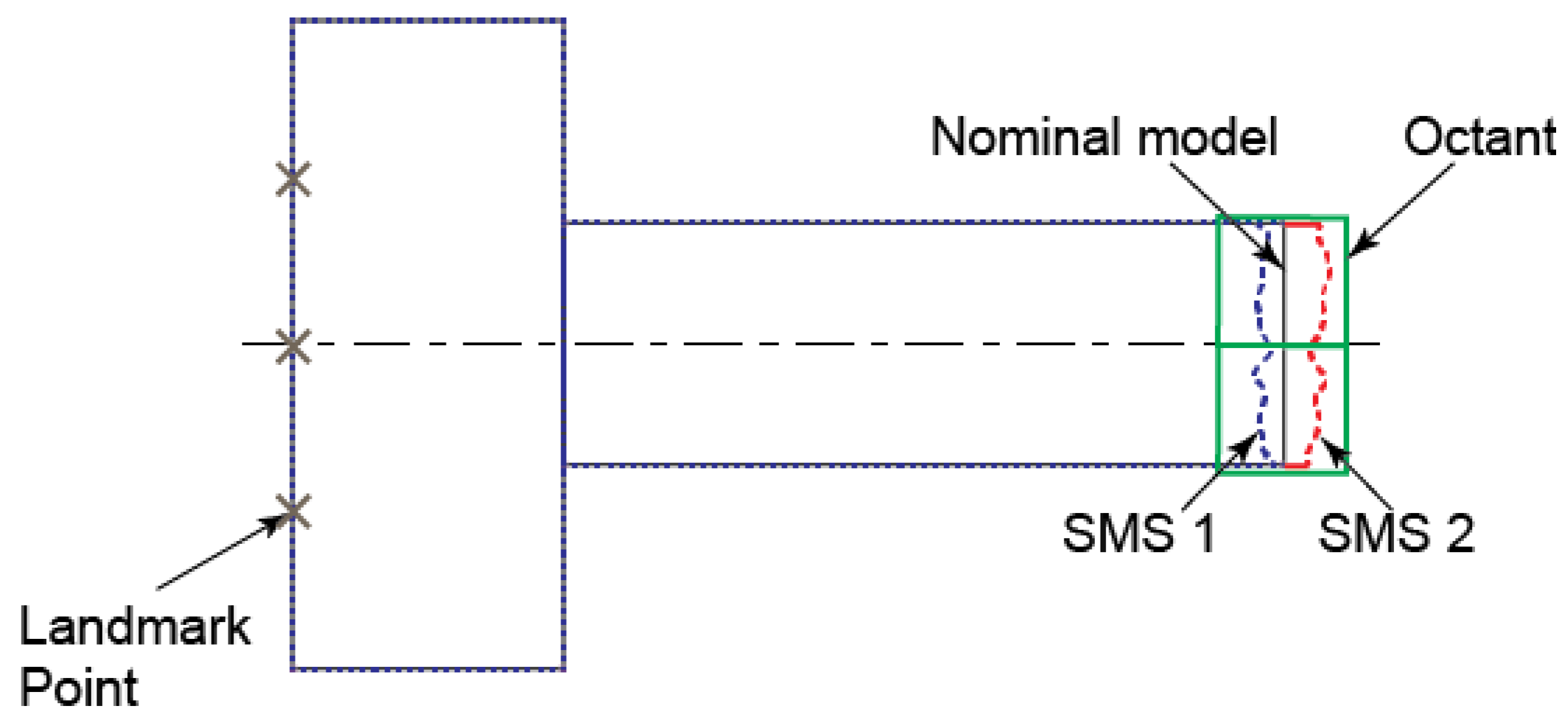
In short, to generate a parametric SMS, multiple SMS are superimposed by registering them at their corresponding landmarks, as shown Figure 4. This pushes the variation away from the landmark feature to other features. Then the collection of mean, min and max points are used to generate a parametric SMS model.
4.2. Variation Visualization
In addition to shapes’ statistical information, there is a need to improve the geometrical variation visualization techniques to support decision making in the product and process development [11]. To study and visualize the effects of change of the manufacturing process parameters on a part shape has been discussed in [17]. Given the difficulty of visualizing the statistical results along the shape surfaces under study, via plots like boxplots, Castillo and Colosimo [17] used projected arrows from surface edges. In this paper, we extend their idea, by locating the bases of cones at the mean points in each octant. The normalized area of the cones can be used to indicate the standard deviation, and the color as the capability index values (this option can be reversed or combined as needed). A single SMS, thus, can be used to visualize variation along the manufacturing and variation information reflected on the cone size and color.
Furthermore, variation visualization often requires the interpretation of deviations from the nominal model or from other SMSs, which may not have vertices perfectly aligned along the desired direction. Hence, the visualization of deviations in an SMS requires the comparison of an unaligned and unequal number of points in the reference model. For this purpose, deviation visualization using Hausdorff distance is suitable for the comparison of two shapes with an unequal number of points, such as the nominal model and SMSs, or between two SMSs. Hausdorff distance is the largest distance between closest points in the neighborhood of a point and is mathematically defined as:
where and are reference and measured data points, respectively.
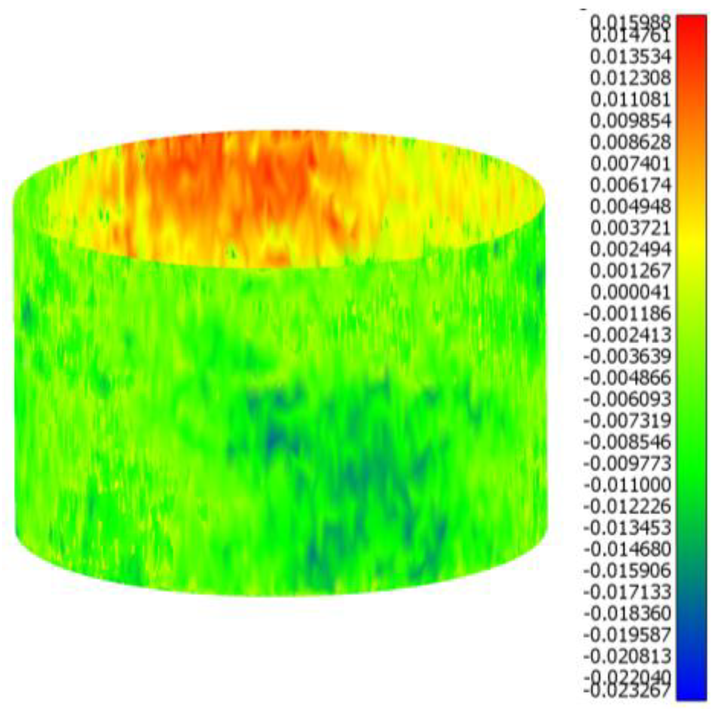
Using Octrees, Hausdorff distance can be computed with a sphere centered at reference point in an octant, which includes all points in neighboring octants; this way all points are compared, and computational time is significantly reduced relative to comparing all points in and [9]. Figure 5 shows the color difference between two SMSs based on Hausdorff distance.
5. Prediction Stage
The prediction of geometrical characteristics of SMSs, in the context of manufacturing, requires the simulation and generation of a would be shape of an actual product. A simulated shape is selected as the predicted SMS once the resulted variation meets a tolerance specification [29]. The predicted SMS contains variation information of the surface, which can also be treated as a variation model.
Research related to variation modelling often focuses on the mathematical modelling of geometrical variation, which is a non-trivial task given the need to consider all form errors [11]. Moreover, major variation propagation modelling techniques, through the use of stream of variation models such Differential Motion Vectors, Equivalent Fixture Error and Kinematic Analysis, consider only the positional and orientation aspects of fixture and datum errors [20]. A manufacturing simulation, however, has the potential to include form errors in addition to position and orientation errors. Variation modelling using manufacturing simulation is an alternative approach when SMS generation is in its later stages [30]. This can be achieved through Boolean operations, in line with the principles of Constructive Solid Geometry (CSG), where the tool profile that perforates a solid model determines the machined surface of the model.
5.1. Machine Tool Setup
A workpiece/stock is setup on a machine tool for machining, which can be considered a pair in the assembly of parts. The resulting assembly will set the part with errors that contain systematic and random errors. The random errors (roughness and waviness) are similar to geographic terrains and the average roughness has no practical meaning in relating surfaces to its functional effectiveness [31]. Further, the surface waviness under a large applied force (such as clamping and cutting forces) has a negligible contribution to the resulting surface variation at a distance greater than 20 mm away from the source, in accordance to Saint-Venant’s Principle [32]. Hence, a manufacturing simulation during the prediction stage can focus only on systematic errors when assembling fixture and part models, without significantly influencing the setup accuracy. In the case of prediction using a stock obtained from observed data, either Wavelet or Laplacian filters can be used to remove the random errors.
5.2. Multistage Manufacturing Simulation
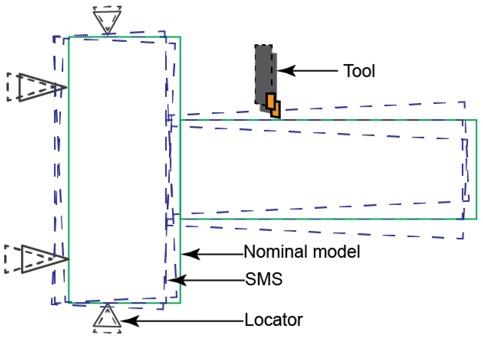
Many manufactured parts pass through multiple stages of production before use in their final applications. A corresponding simulation should follow this type of production. In a multistage production, a machining feature becomes an assembly feature in subsequent stages, in relation to the fixture or tolerancing surface, as shown in Figure 6. Moreover, the total geometric error of a part can be attributed to machine tool errors (machine tool deflection under load—due to clamping and cutting force, cutting-tool wear, thermal errors, kinematics error, spindle motion, and controller errors), work-piece geometric and thermal errors, and fixture errors [33]. The combinatorial nature of those errors and interdependence between multiple stages makes the prediction of the final parts’ geometric characteristics a non-trivial task. However, since the main interest in predicting SMSs is for tolerance design and analysis and not necessarily studying the effects of each of the parameters, the cumulative effect of those sources of error on the manufactured part can be studied collectively.
Therefore, the sources of error are decoupled and grouped into machining tool error (cumulative error reflected at the cutting-tool tip), workpiece geometrical error (datum error, induced in previous station), and fixture error [33]. The effect of these errors on manufactured parts are expressed as deviations from the expected or nominal surfaces, which can safely be captured by range of deviation values per octant. Those deviations are mimicked by introducing errors to a fixture-workpiece assembly and toolpath trajectory during manufacturing simulation. When a prototype is available, these values are iteratively updated, otherwise, they are assumed from experience or deducted from the process capability when known in priori.
Since the main interest of SMS generation is in performing tolerance analysis, the range of possible SMS can be generated by experimenting with deviation values so that the simulation result falls within a reasonable range. This requires experimenting with a multiple range of deviation values. Design of Experiments (DOE) is an ideal tool for the economical generation of a combination of a range of values, studying the effects of change of those values.
Using a full factorial approach, the collection of worst-case points per octant and range of machine tool parameters for a given fixture error can be used to generate parametric SMSs. By tweaking these values, an initial range of promising SMSs can be generated. The experiments are iteratively updated until the simulation results fall within a specified tolerance zone. It is worth noting that the deviations are small enough that a linear change between the two levels of the factors can be assumed without compromising the accuracy of the prediction. Moreover, the advantage of following this approach is that the required number of experiments does not increase with the number of samples per station, as the samples are reduced to a parametric SMS. The resulting parametric SMS is then used in subsequent stations. Once a simulation is completed, topological characteristics are added using Gaussian random fields or Fractal surfaces [34]. Currently, to the best of our knowledge, there are no CAx tools to support this methodology; hence, the development of such tools towards automating the experiments would expedite the prediction process.
Furthermore, using this approach, each experiment, with given factors, produces a specific SMS response. These can be used to map error sources to part the geometric characteristics and study the effect of manufacturing factors on the resulting shape. Figure 7 illustrates some of the possible effects of locator deviations on the orientation of a model, along with tooltip deviation; by simulating all combinations of these deviations for a given model, the geometric characteristics of a part can be predicted. Once the predicted geometric characteristics approach actual geometric data, the iteratively estimated collection of errors at each stage can then be used as a variation propagation model of the manufacturing line.
5.3. Adding Random Deviations
Once the range of manufacturing error values are determined by the iterative process presented above any error values within this range can be used to simulate instances of shapes with systematic deviations. The systematic deviations represent position and orientation errors and do not contain form errors. Often, form errors are distributed haphazardly along the surface of a feature. Hence this random distribution can be characterized with Gaussian random fields, which can then be added to the surface with systematic deviations. A similar approach has been discussed in [4,35].
For simpler cases of a horizontal plane feature, where the number of points in both surfaces are equal and have the same x and y values, the corresponding z values can be added together, as shown in Figure 8. Nevertheless, when the number of points is not equal, interpolation like a trilinear interpolation per octant can be applied to add Gaussian random fields to the systematic deviations. Mathematically, let be point cloud of systematic deviation and be the point cloud of random deviation, where is the total number of points; the total deviation can be expressed as:
6. Observation Stage
6.1. Homologous Data Points
In the observation stage, measurement data is collected and GeoSpelling operations, such as segmentation, filtering, and extraction, are performed [4]. Further, a variation analysis can also be performed with the help of SSA, which includes the extraction of the variation envelope and standard deviation per octant, thereby generating a parametric SMS. To perform SSA, the homologous features and points of superimposition of SMSs must be aligned. However, given that octants are cube shaped, when multiple SMS are superimposed, the variation range can get larger than the octant lengths, which may put homologous data points in separate octants.
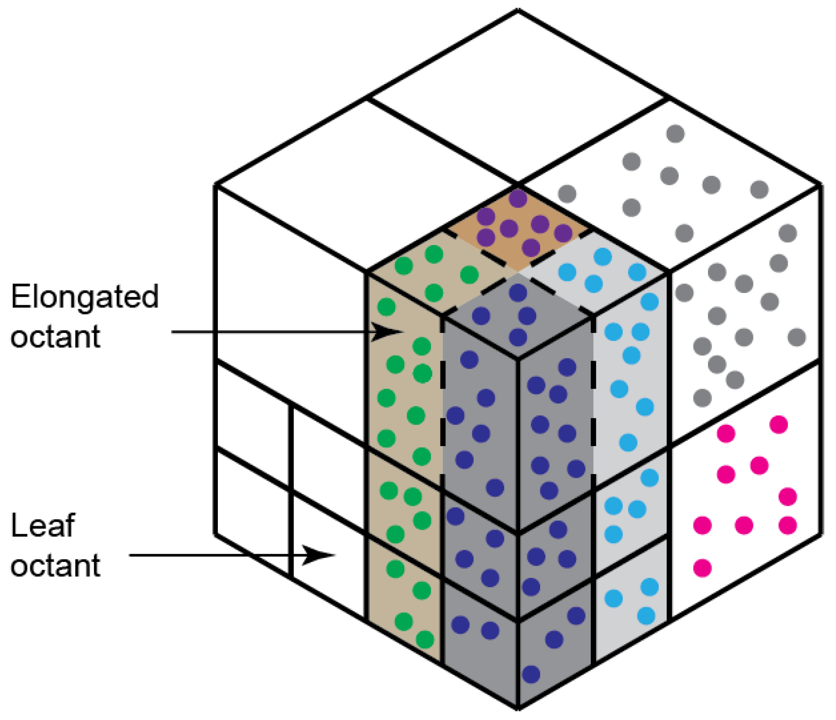
Thus, to group all points of a region from each SMS in a single octant, the length of octants needs to be elongated in one direction. Each leaf octant is elongated by stretching the smallest octant of the neighboring octants in the direction of the desired dimensional analysis, to meet the bounding box. This insures all points in the direction of interest are included in one octant, creating a rectangular prism. The number of elongated-octants becomes fewer than the initial number of octants as the result of removing the parent octants, which may improve computational efficiency in subsequent operations. Figure 9 shows elongated leaf octants and their occupants. Figure 10 shows the sequence of elongating leaf octants up to the boundaries of a root node and Algorithm 1 presents a pseudocode to generate elongated-octants along their corresponding occupant points. Mathematically, let all vertices of an Octree with octants and where is normal to the plane of interest, the projected vertices of the octree become:
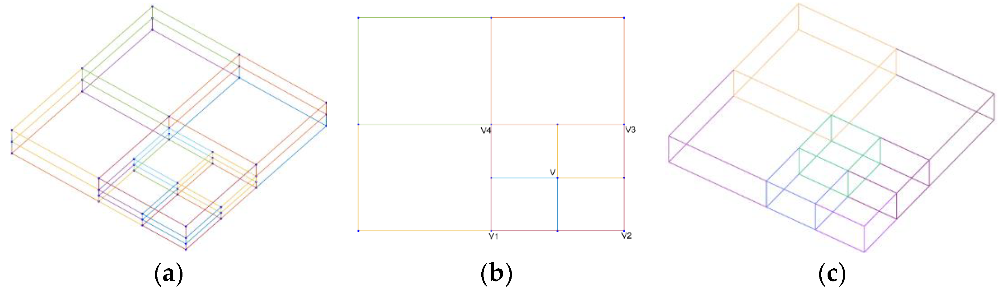
The non-leaf octants can be culled by checking if an octant includes one or more vertices. For instance, for an octant with vertices shown in Figure 10b, the occurrence of vertex V indicates the encapsulation of the leaf octants. This can be expressed as:
where projected vertices encapsulate an octant with a vertex when .
A similar approach can be applied in determining if data points are encapsulated within projected vertices. Furthermore, for a given Octree bounding box the projected vertices of leaf octants to the bounding box can be obtained by:
Then the vertices of elongated octants become the concatenation of the previously projected vertices and the vertices projected to the bounding box.
| Algorithm 1 Pseudocode to generate elongated-octant and assign corresponding occupants |
| 1: Input: Octants’ vertices, 2: Output: elongated-octants, , occupant points in 3: function GenerateElongatedOctants () 4: ← Project in direction of plane of interest 5: for each in do 6: ← Remove if encapsulates other 7: end 8: ← Project to root node’s boundaries 9: ← generate an elongated-octant with 10: <, > ← Collect in 11: return <, P> 12: end |
6.2. Surface Reconstruction
The representation of non-ideal surfaces within CAD tools for application in Computer-aided tolerance analysis, finite element analysis, and assembly simulation is of high importance (e.g., [15,16]). Thus, the parametric SMS generated with the help of elongated-octants should be integrated with a CAD surface for further analysis. Observed point cloud data can be converted to CAD surfaces by generating and transforming NURBS surfaces to any supported CAD formats, such as IGES [15]. Using Octrees, a surface reconstruction technique, known as Screened Poisson Surface Reconstruction (SPSR) [10], can be used to generate water-tight mesh from measured data points. Using SPSR, surfaces are constructed by B-spline surfaces by using algorithms that combine the surfaces constructed separately within an octant and collectively using all data points. Using the technique, a high accuracy surface, at a high computational efficiency, can be generated. However, SPSR is sensitive to noise and outliers [10]; thus, GeoSpelling operations such as filtering and outlier culling must be performed prior to proceeding with SPSR.
7. Tolerance Analysis
Assembling of multiple SMSs is a practical approach to perform 3D stack up tolerance analysis. To assemble SMSs, a constrained registration approach or difference surface approach can be applied [36]. To perform tolerance analysis, meshes of features of interest are scaled to a specified tolerance or manufacturing variation range. Using Octrees, each point is allowed a distance of travel in an elongated octant, depending on the range of a specified or observed data per elongated octant. This approach can be applied in performing the worst-case and statistical tolerance analysis.
7.1. Worst-Case Tolerance Analysis
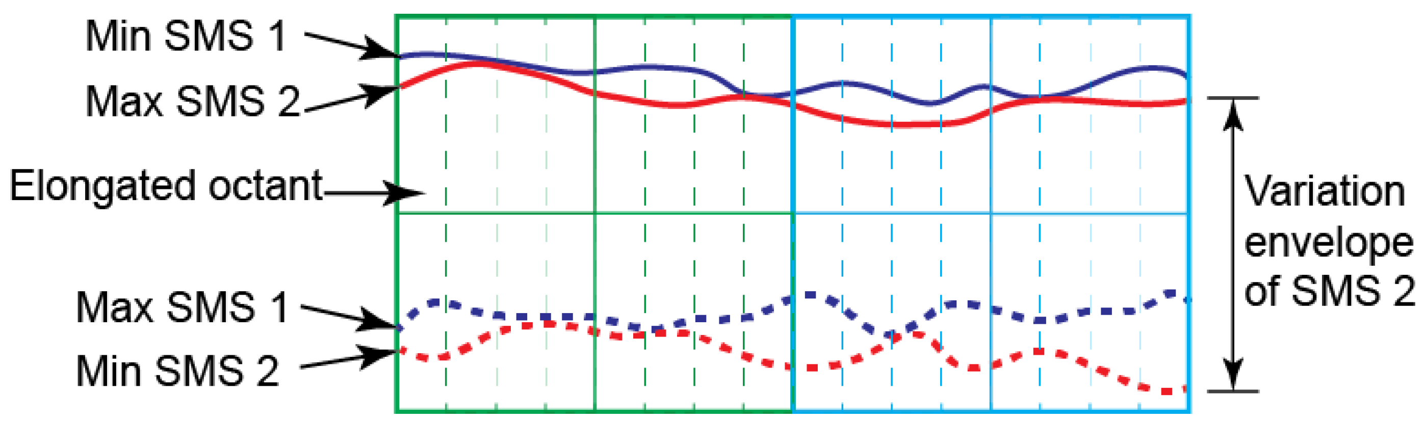
As pointed out, a parametric SMS is a mean shape with geometric variation information. To obtain variation information, all available SMSs are superimposed and mean, min, and max deviation values per elongated-octant, in the direction normal to a nominal surface, are collected. The min and max values are then used to generate multiple SMSs, yielding a variation envelope. Figure 11 illustrates the min and max position of two SMSs per elongated-octant, where the variation zone is unique to each elongated-octant. The mean point positions changed between the min and max value, and the assembly of the set of these shapes is used in performing worst-case tolerance analysis. The worst-case points can be collected using Equation (4).
7.2. Statistical Tolerance Analysis
Worst-case approach is an overly conservative and a highly cautious approach of tolerance analysis. The statistical approach, however, can reduce costs by letting few parts fail to meet design specifications (e.g., [37]). Several statistical techniques have been proposed for non-linear statistical tolerance analysis; the Monte Carlo simulation is a wide spread technique. Monte Carlo uses random value sampled from a statistical distribution associated with a manufacturing process, oftentimes dimensional data. However, using dimensional data overlooks form errors and assigns a single distribution for an entire surface. Using Octrees, each mean point of an elongated-octant uses a separate set of mean and standard deviation values. By the same token, a separate probability distribution can be used for specific regions of a feature. Algorithm 2 shows a Pseudocode to generate position error from nominal assembly. Mathematically, let the set of mean points per elongated octant with index e be ; for a case where variation is in z direction, the new set of points can be expressed as follows:
For a more general case, where variation is in direction of vector , becomes
| Algorithm 2 Pseudocode for implementing Octree-based statistical tolerance analysis |
| 1: Input: elongated-octant’s index e, mean standard dev., 2: Output: position error FR 3: function PositionError (<e, >) 4: Initialize FR 5: for desired number of samples do 6: for each SMS’s surface of interest do 7: ← get new point positions from a normal distribution of <e, ()> 8: end 9: re-assemble all SMSs 10: FR ← Get deviation from nominal assembly and update FR 11: end 12: return FR 13: end |
8. Illustration Case
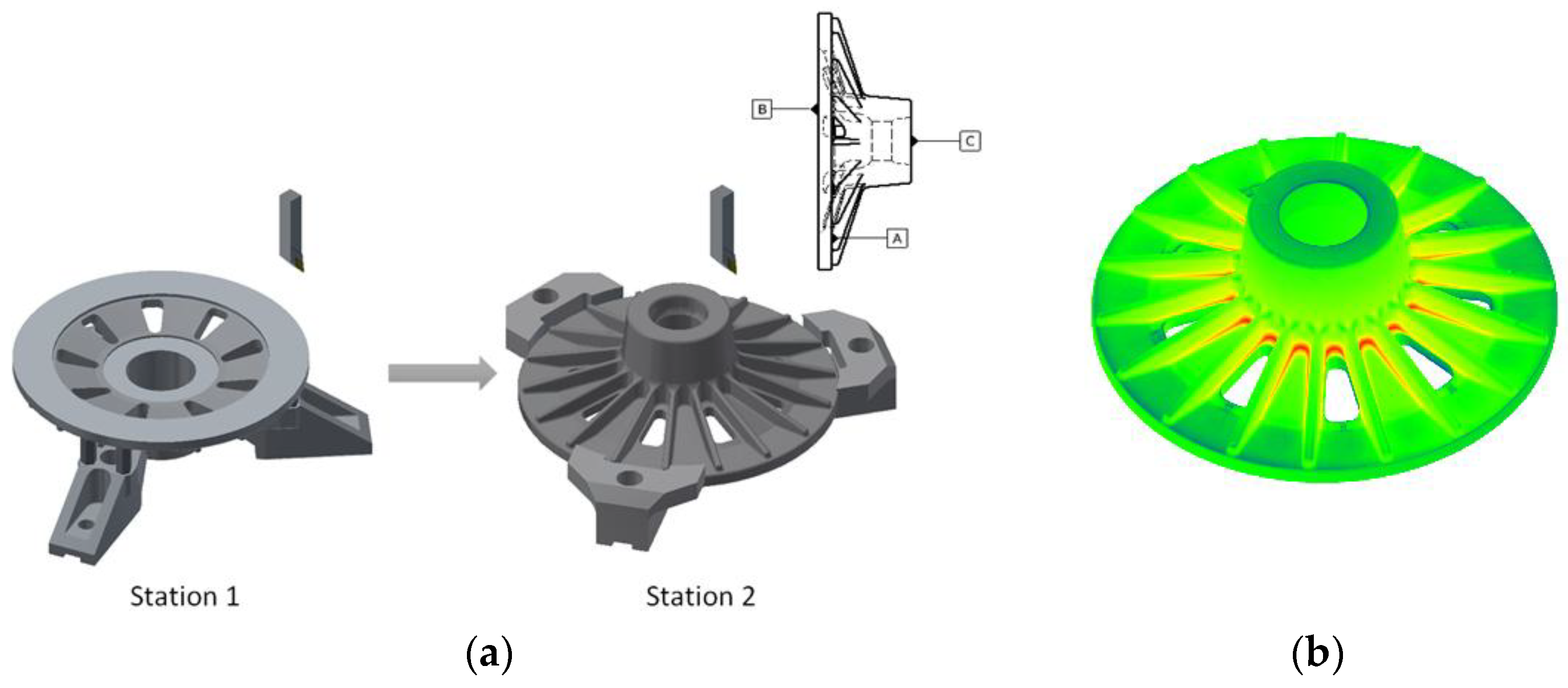
To demonstrate the method, an industrial two-stage truck component manufacturing line was considered, with setups shown in Figure 12. In the first station, a forged blank was used as a stock and feature B was faced by setting up feature A on a fixture. In the second station, feature C was faced by setting up feature B on a fixture. The machined feature C was used to compare the accuracy of prediction with the corresponding scanned model. The implementation of the algorithms presented below were carried out in Matlab 2017b and the CAM simulation in Autodesk Inventor HSM.
8.1. Prediction Stage
As stated, in the above, manufacturing error sources can be grouped into three independent sources: datum, fixture, and tooltip deviations. For illustration, this paper assumes a tooltip deviation in the normal direction to the machining feature and a constant fixture error per batch.
During CAM simulation of the operations for both stations, nominal toolpaths were generated using nominal models assembled to nominal fixtures. Then, in the first station, since there was no acquired SMS to start with; datum and estimated fixture error with a combined parallelism value of 0.5 mm and a tooltip deviation from the nominal path in the direction normal to the surface in the range of −0.2 to −0.4 mm were assumed (the initial assumptions of the deviation values were updated based on observed data). Four simulation experiments were performed following DOE principles and the worst-case SMSs were extracted. Then, the worst-case SMSs from station 1 were used as a stock to station 2 by following the series of experiments shown in Table 1. The result obtained shows that the predicted response of the mean shape points are within the 0.002 mm range of the mean value of the observed data. The difference between individual samples of the observed data and the predicted result was used to conjecture the error source that could have caused the difference. Moreover, the feature C’ error due to datum deviation was smaller than the depth of cut; hence resulting in a similar response for both worst-cases for a given tooltip deviation, as shown in Table 1. Nevertheless, the effect of the datum error was visible on the internal and external cylinders of the neck of the model.
8.2. Observation Stage
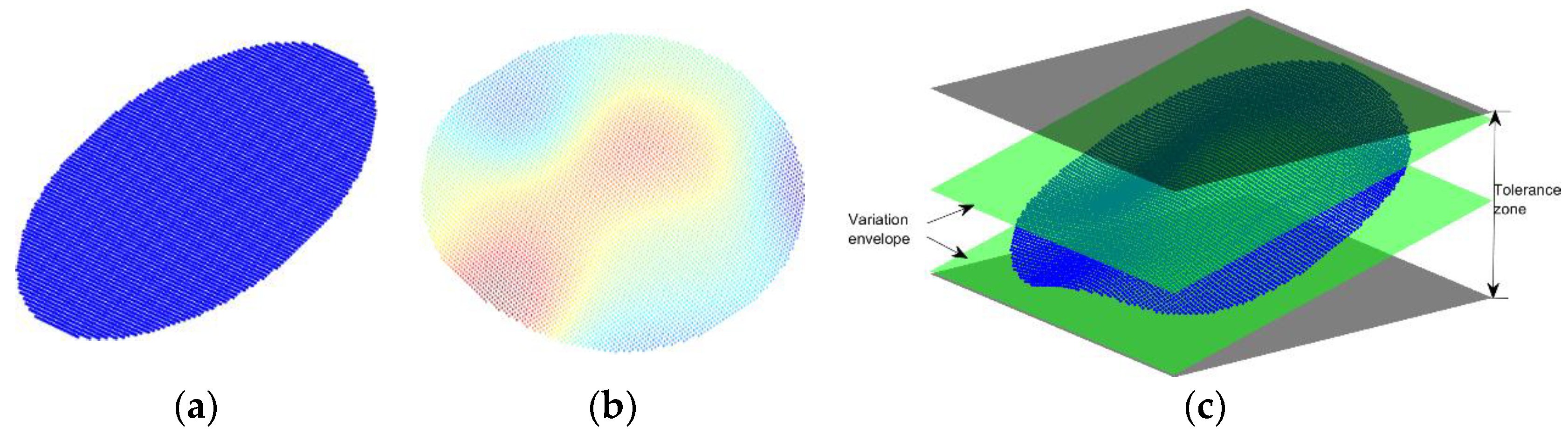
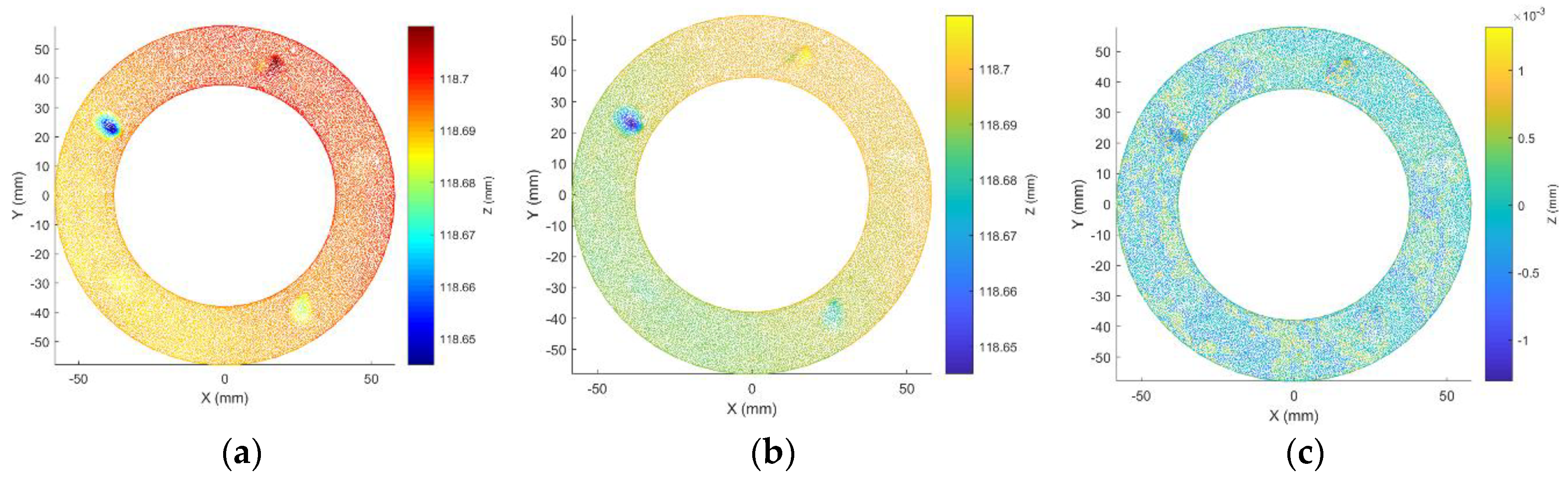
An optical scanner, ATOS Triple Scan™, Braunschweig, Germany, with resolution up to of 5 microns and space between points up to 0.01 mm was used to obtain 5 samples produced from each station, at an average of 4.7 million points per sample. From each of the sample features A, B, and C were partitioned out for variation analysis. Furthermore, since SPSR is sensitive to noise and outliers, the wavelet filtering technique was used to remove random errors from each sample, as shown in Figure 13. Outlier points were filtered out from the samples by extracting the inlier points of the best fitting planes. Parallelism of features A and B were used to iteratively update the assumed fixture error during the prediction stage and feature C was used to study the manufacturing effect from the two stages.
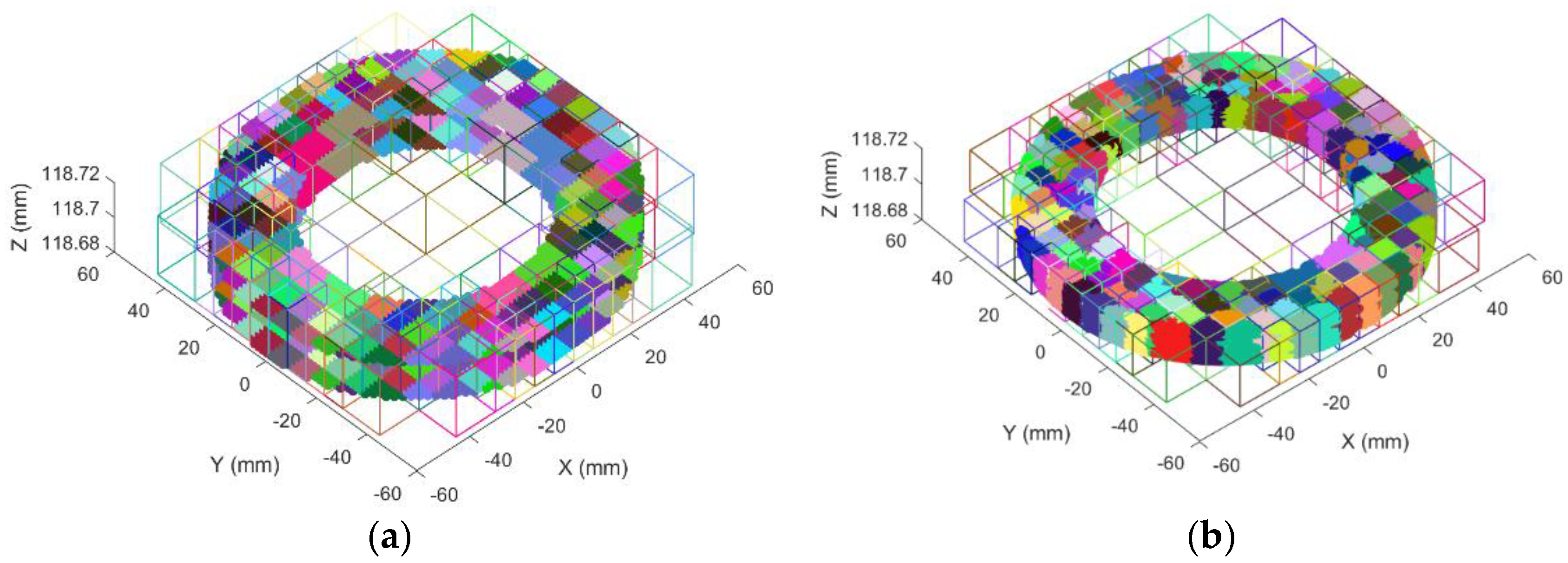
First, to perform the variation analysis, five samples of feature C were superimposed and partitioned by an Octree. A set of 500 points per octant were used to generate the leaf octants, from which elongated-octants were generated, as shown in Figure 14. As a result, the number of octants was reduced from 335 to 265. Then, using the elongated-octants, the means of points per SMS per elongated-octant were extracted to determine the mean shape and worst-case SMSs.
Further, the superimposed samples had heights below the nominal height of feature C; i.e., 118.75 mm, with variation range of 0.02 mm. This variation was attributed to the tooltip deviation rather than a fixture or datum error. The simulation result showed that the contribution of fixture error was parallel to the surfaces and resulted in a constant standard deviation throughout all regions of surfaces; this indicated that there was a pattern consistent in all the samples, as shown in the simulation result in Figure 14a. However, there was no noticeable pattern of orientation in the actual surface of all the samples. This could be attributed to the unbalanced clamping force, which was set manually based on the operator’s experience.
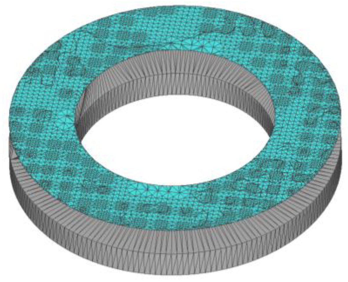
Moreover, the collection of mean points of the mean shape with their normal vectors were used to construct a surface using the SPSR technique at an Octree depth of 10. The reconstructed surface dependence on the Octree level creates a fine mesh around the mean points and a course mesh in the space between the points. Boolean operations were performed to modify the reconstructed surface to the dimensions of the solid model of the part, as shown in Figure 15. Similarly, the surface could also be reconstructed from the collection of min or max points.
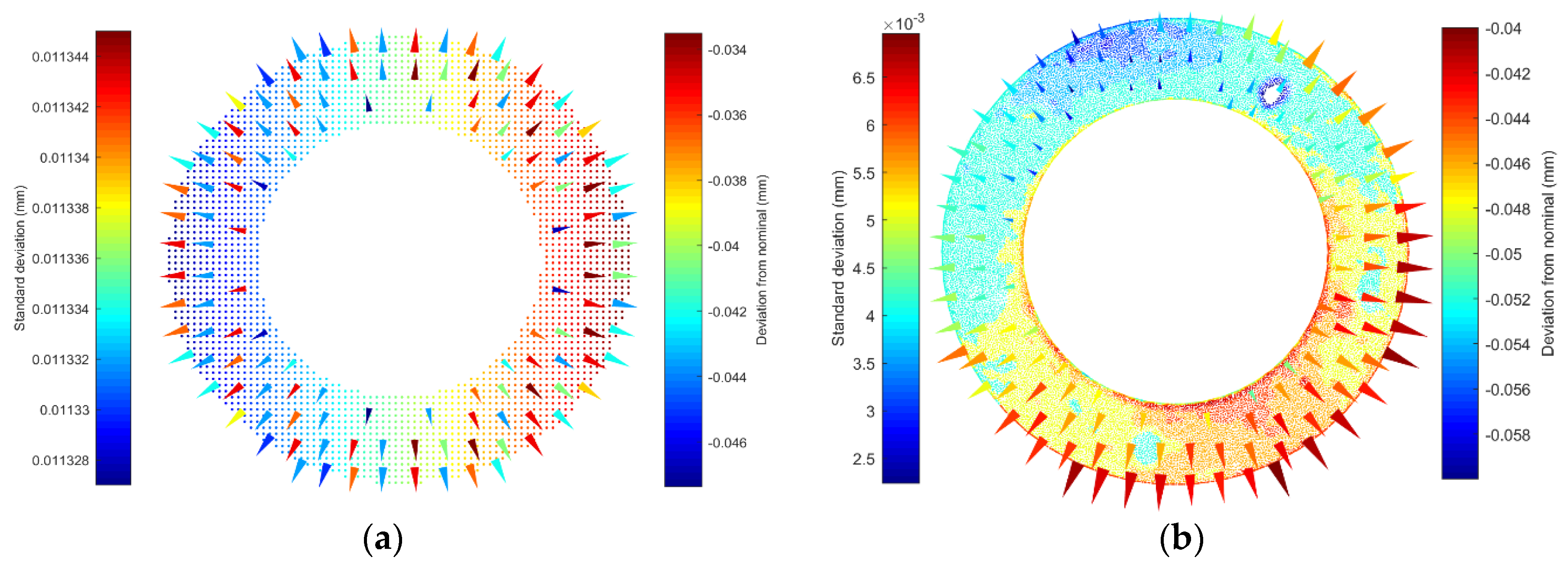
To visualize variation, a set of cones at the mean shape points were placed, with cone size and color indicating standard deviation values. These values were extracted by computing the mean and standard deviation of mean points per SMS per elongated-octant. A sample in Figure 16b shows a variation larger on one side than the other, which, as stated in the above, could be attributed to the unbalanced clamping force. Further, Matlab’s coneplot function was applied to generate the cones.
8.3. Tolerance Analysis
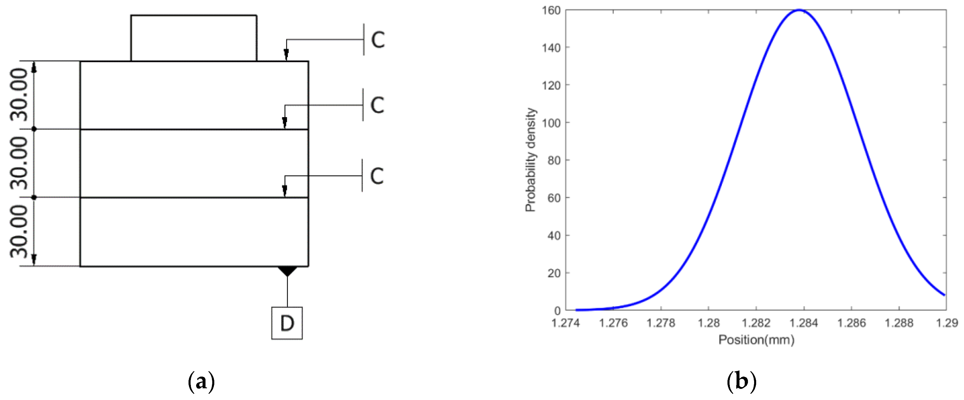
To illustrate the method’s application in tolerance analysis, two hallow cylinders were stacked at the top each other through a shaft; the top and bottom surfaces were constructed from the mean shape of feature C’s observed data, as shown in Figure 17a. The cylinders were assembled using the constrained registration approach [36]. For worst-case tolerance analysis, the mean shape points were displaced to min and max deviation positions at each octant to obtain worst-case SMSs. The maximum position error of 1.33 mm was obtained. For statistical tolerance analysis, each octant used different sets of mean and standard deviation values (using values shown in Figure 16b) to generate point positions from a Gaussian distribution. Figure 17b shows position error from the nominal assembly position that was generated from 1000 simulations.
8.4. Comparison of Computational Efficiency
To illustrate the computational advantages of using Octree, a point cloud of the industrial product shown in Figure 12b, with a file size of 370 MB and around 4.7 million points, was first converted to .stl and .obj file formats. We experimented with the Octree-based reconstruction approach using the SPSR technique implemented in MeshLab, an open source system, with an Octree depth of 8. Surface reconstruction using SPSR took 15 s to pre-clean and reconstruct the surface, with working memory reaching up to 50 MB. On the other hand, two B-Rep based commercial CAD tools, Autodesk Inventor 2017 and Solidworks 2016, were unable to parse the files due to too many surfaces. The experiment was repeated with a partitioned point cloud shown in Figure 13a, with 23,000 points, which took 5 s in MeshLab and about 2.5 min to convert to a surface model in both Autodesk Inventor and Solidworks. The experiment was performed in a 2.8 GHz Intel Core i7-4810MQ CPU machine with a 32 GB RAM and Windows 7 operating system. This shows that the Octree-based reconstruction of surfaces from point cloud data is much faster than performing similar operation in CAD tools.
9. Discussion
As it has been pointed out, octree has the advantages of computational efficacy and the ability of partitioning SMSs into small regions. It has been shown that Octree-based reconstruction of surfaces, using SPSR, from point cloud data is much faster than performing a similar operation in CAD tools. The slow time in CAD tools could be due to the solid modeling tools apply boundary representation technique, which requires numerous boundary surfaces to be constructed to represent an SMS. Moreover, the speed of Octree-based data processing is dependent on the number of octants (Octree depth). In performing a variation analysis, the number of Octants is reduced as the result of Octree-elongation. Hence, the computational efficiency of performing variation analysis using octants in likely to be better than regular grid-based approaches. It is a generally accepted notion that construction of Octree itself exhibits the time complexity of , which is insignificant in terms of memory consumption during runtime for . This is in line with the results of the experiments on computational efficacy of Octrees in processing a large amount of point cloud data, as reported in [9,38,39].
Furthermore, this work applied CAM simulation to predict the geometrical deviations due to manufacturing errors. For this purpose, any kind of CAM simulation tool can be applied. Nevertheless, Octree-based CAM simulation approaches are better than the widely used commercial B-Rep based modelling and simulation tools in computational efficiency. For instance, comparing a 3-axis milling simulation using a ball-end mill in the B-Rep based solid modeling tool, the octree-based CAM simulation performed 54 times faster and consumed around 14% of the working memory consumed by the B-Rep based simulation, at an accuracy better than 1 micron [6]. Similar results have also been reported in [5].
The approach attempts to relate manufacturing errors to the geometric deviation of parts by iteratively experimenting with toolpath and fixture deviations until the feature of interest falls within a specified tolerance or manufacturing variation. The manufacturing errors are specifically pointed out by visualizing how close the orientation and position of the simulated feature is relative to the scanned ones. It is worth noting that on successful approximation of the source of the deviation values from the given samples, by following the above approach, a variation propagation model for a manufacturing line can be generated. The same technique could also be applied for more complex parts. This would reduce the profound mathematical understanding required in the modeling of geometric variations of complex shapes as discussed in [11]. However, the CAM simulation-based approach may take time in manually setting up the SMSs in simulation environments that are capable of inducing fixture and toolpath errors.
Moreover, a variation analysis based on elongated-octants that encapsulate SMSs or specific regions of interest was applied. The elongated-octant based approach can be extended in the line of thinking presented in [40,41], where SMSs are encapsulated in a reference box and variation analysis is performed thereon. However, the weakness of our approach is that the collection of mean, min, and max points that make a new SMS were treated as independent points, which may give an unrealistic shape. Further investigation is required to determine the correlation among these points.
Despite the computational advantages, Octree-based generation of SMSs require a separate environment from the prevalent B-Rep based CAD tools. This would necessitate the manipulation of SMSs to be performed in an octree-based environment and later results reported back to a B-Rep based environment. Application programming interfaces (APIs) may be applied in exchanging data to and from both environments. Upon successful implementation of SMS related algorithms in an Octree-based environment, the computational issues are likely to be improved significantly.
10. Conclusions
This paper attempted to show how Octrees can be applied in the generation and variation analysis of Skin Model Shapes. Specifically, the paper aimed towards addressing some of the existing research challenges, such as the development of methods for geometrical data processing, mapping of manufacturing error sources to geometric models, and improvement of variation visualization techniques. Octrees, for their computational efficiency and advantage of localizing manufacturing signatures, were applied in geometrical data processing, such as extracting mean, min, max, and standard deviation values, deviation visualization and surface reconstruction. Further, Octrees were applied in the prediction and observation stages of SMS generation for extracting the worst-case SMSs and in performing associated tolerance analysis. This paper also showed how manufacturing source of errors can be mapped to part geometric characteristics with the help of Octrees, CAM simulations, and Design of Experiments. This includes running multiple experiments that combine datum errors and tooltip deviations for a given fixture error. Furthermore, often a single SMS’s deviations from nominal model are studied one at a time, ignoring other SMS products of the same batch; this paper introduced a cone-based standard deviation visualization approach to study the range of variation of all SMSs along with the deviations from a nominal model.
This work can be extended by decomposing the factors that affect the toolpath trajectory into subcomponents such as thermal and kinematic errors, thereby getting a more accurate prediction of SMSs. Further, the elongated octants that were used to collect and perform a variation analysis on homologues points focused on a plane feature. For features other than the plane feature, approaches like Ray casting [42] on octants will be investigated in future works.
Author Contributions
Conceptualization, Methodology, Writing-Original Draft Preparation, F.Y.; Supervision, Writing-Review & Editing, Funding Acquisition, D.S.; Data Curation, Resources, Project Administration, D.S. and E.N.
Funding
This research was funded by PRIZE project, VINNOVA, Sweden, Diar. nr. 2016-03303 under Produktion2030 program.
Acknowledgments
The authors thank VINNOVA and the Produktion2030 program for supporting the project.
Conflicts of Interest
The authors declare no conflict of interest.
References
- Geis, A.; Husung, S.; Oberänder, A.; Weber, C.; Adam, J. Use of vectorial tolerances for direct representation and analysis in CAD-systems. Procedia CIRP 2015, 27, 230–240. [Google Scholar] [CrossRef]
- Ballot, E.; Bourdet, P.; Thiébaut, F. Determination of relative situations of parts for tolerance computation. In Geometric Product Specification and Verification: Integration of Functionality; Springer: Dordrecht, The Netherlands, 2003; pp. 63–72. [Google Scholar]
- Davidson, J.K.; Shah, J.J.; Mujezinović, A. Method and Apparatus for Geometric Variations to Integrate Parametric Computer-Aided Design with Tolerance Analysis and Optimization. U.S. Patent 6,963,824, 8 November 2005. [Google Scholar]
- Schleich, B.; Anwer, N.; Mathieu, L.; Wartzack, S. Skin Model Shapes: A new paradigm shift for geometric variations modelling in mechanical engineering. CAD Comput. Aided Des. 2014, 50, 1–15. [Google Scholar] [CrossRef]
- Erdim, H.; Sullivan, A. Cutter workpiece engagement calculations for five-axis milling using composite adaptively sampled distance fields. Procedia CIRP 2013, 8, 438–443. [Google Scholar] [CrossRef]
- Sullivan, A.; Erdim, H.; Perry, R.N.; Frisken, S.F. High accuracy NC milling simulation using composite adaptively sampled distance fields. CAD Comput. Aided Des. 2012, 44, 522–536. [Google Scholar] [CrossRef]
- Koschier, D.; Deul, C.; Bender, J. Hierarchical hp-Adaptive Signed Distance Fields. In Proceedings of the ACM SIGGRAPH/Eurographics Symposium on Computer Animation, Zurich, Switzerland, 11–13 July 2016; pp. 189–198. [Google Scholar]
- Maréchal, L. Advances in octree-based all-hexahedral mesh generation: Handling sharp features. In Proceedings of the 18th International Meshing Roundtable, Salt Lake City, UT, USA, 25–28 October 2009; Springer: Berlin/Heidelberg, Germany, 2009; pp. 65–84. [Google Scholar] [CrossRef]
- Girardeau-Montaut, D.; Roux, M.; Marc, R.; Thibault, G. Change detection on points cloud data acquired with a ground laser scanner. Int. Arch. Photogramm. Remote Sens. Spat. Inf. Sci. 2005, 36, W19. [Google Scholar]
- Kazhdan, M.; Hoppe, H. Screened poisson surface reconstruction. ACM Trans. Graph. 2013, 32, 1–13. [Google Scholar] [CrossRef] [Green Version]
- Schleich, B.; Wartzack, S. Challenges of Geometrical Variations Modelling in virtual Product Realization. Procedia CIRP 2017, 60, 116–121. [Google Scholar] [CrossRef]
- Schleich, B.; Wartzack, S. Tolerance Analysis of Rotating Mechanism Based on Skin Model Shapes in Discrete Geometry. Procedia CIRP 2015, 27, 10–15. [Google Scholar] [CrossRef]
- Schleich, B.; Wartzack, S. A Quantitative Comparison of Tolerance Analysis Approaches for Rigid Mechanical Assemblies. Procedia CIRP 2016, 43, 172–177. [Google Scholar] [CrossRef]
- Schleich, B.; Wartzack, S. Evaluation of geometric tolerances and generation of variational part representatives for tolerance analysis. Int. J. Adv. Manuf. Technol. 2015, 79, 959–983. [Google Scholar] [CrossRef]
- Zhang, Z.; Zhang, Z.; Jin, X.; Zhang, Q. A novel modelling method of geometric errors for precision assembly. Int. J. Adv. Manuf. Technol. 2018, 94, 1139–1160. [Google Scholar] [CrossRef]
- Yan, X.; Ballu, A. Generation of consistent skin model shape based on FEA method. Int. J. Adv. Manuf. Technol. 2017, 92, 789–802. [Google Scholar] [CrossRef]
- Castillo, E.; Colosimo, B.M. Statistical Shape Analysis of Experiments for Manufacturing Processes. Technometrics 2011, 53, 1–15. [Google Scholar] [CrossRef]
- Zhang, M. Discrete Shape Modeling for Geometrical Product Specification: Contributions and Applications to Skin Model Simulation. Ph.D. Thesis, École Norm supérieure Cachan-ENS, Cachan, France, 2012. [Google Scholar]
- Matuszyk, T.I.; Cardew-Hall, M.J.; Rolfe, B.F. The kernel density estimate/point distribution model (KDE-PDM) for statistical shape modeling of automotive stampings and assemblies. Robot. Comput. Integr. Manuf. 2010, 26, 370–380. [Google Scholar] [CrossRef]
- Yang, F.; Jin, S.; Li, Z. A comprehensive study of linear variation propagation modeling methods for multistage machining processes. Int. J. Adv. Manuf. Technol. 2017, 90, 2139–2151. [Google Scholar] [CrossRef]
- Keum, Y.T.; Ahn, I.H.; Lee, I.K.; Song, M.H.; Kwon, S.O.; Park, J.S. Simulation of stamping process of automotive panel considering die deformation. AIP Conf. Proc. 2005, 778, 90–95. [Google Scholar] [CrossRef]
- Ibaraki, S.; Yoshida, I. A five-axis machining error simulator for rotary-axis geometric errors using commercial machining simulation software. Int. J. Autom. Technol. 2017, 11, 179–187. [Google Scholar] [CrossRef]
- Sato, R.; Sato, Y.; Shirase, K. Finished Surface Simulation Method to Predicting the Effects of Machine Tool Motion Errors. Int. J. Autom. Technol. 2014, 8, 801–810. [Google Scholar] [CrossRef]
- Siraskar, N.; Paul, R.; Anand, S. Adaptive Slicing in Additive Manufacturing Process Using a Modified Boundary Octree Data Structure. J. Manuf. Sci. Eng. 2015, 137, 011007. [Google Scholar] [CrossRef]
- Vo, A.; Truong-hong, L.; Laefer, D.F.; Bertolotto, M. Octree-based region growing for point cloud segmentation. ISPRS J. Photogramm. Remote Sens. 2015, 104, 88–100. [Google Scholar] [CrossRef]
- Lee, K.H.; Woo, H.; Suk, T. Point Data Reduction Using 3D Grids. Int. J. Adv. Manuf. Technol. 2001, 18, 201–210. [Google Scholar] [CrossRef]
- Del Castillo, E. Statistical Shape Analysis of Manufacturing Data. In Geometric Tolerances; Springer: London, UK, 2011; pp. 215–234. [Google Scholar] [Green Version]
- Shah, J.J.; Ameta, G.; Shen, Z.; Davidson, J. Navigating the Tolerance Analysis Maze. Comput. Aided Des. Appl. 2007, 4, 705–718. [Google Scholar] [CrossRef]
- Anwer, N.; Schleich, B.; Mathieu, L.; Wartzack, S. From solid modelling to skin model shapes: Shifting paradigms in computer-aided tolerancing. CIRP Ann. Manuf. Technol. 2014, 63, 137–140. [Google Scholar] [CrossRef]
- Yan, X.; Ballu, A. Toward an Automatic Generation of Part Models with Form Error. Procedia CIRP 2016, 43, 23–28. [Google Scholar] [CrossRef]
- Stout, K.J.; Liam, B. Three Dimensional Surface Topography; Elsevier: London, UK, 2000. [Google Scholar]
- Guo, J.; Li, B.; Liu, Z.; Hong, J.; Wu, X. Integration of geometric variation and part deformation into variation propagation of 3-D assemblies. Int. J. Prod. Res. 2016, 54, 5708–5721. [Google Scholar] [CrossRef]
- Abellán-Nebot, J.V.; Subirón, F.R.; Mira, J.S. Manufacturing variation models in multi-station machining systems. Int. J. Adv. Manuf. Technol. 2013, 64, 63–83. [Google Scholar] [CrossRef] [Green Version]
- Armillotta, A. Tolerance Analysis Considering form Errors in Planar Datum Features. Procedia CIRP 2016, 43, 64–69. [Google Scholar] [CrossRef]
- Liu, J.; Zhang, Z.; Ding, X.; Shao, N. Integrating form errors and local surface deformations into tolerance analysis based on skin model shapes and a boundary element method. CAD Comput. Aided Des. 2018, 104, 45–59. [Google Scholar] [CrossRef]
- Schleich, B.; Wartzack, S. Approaches for the assembly simulation of skin model shapes. CAD Comput. Aided Des. 2015, 65, 18–33. [Google Scholar] [CrossRef]
- Nigam, S.D.; Turner, J.U. Review of statistical approaches to tolerance analysis. Comput. Des. 1995, 27, 6–15. [Google Scholar] [CrossRef]
- Elseberg, J.; Borrmann, D.; Nüchter, A. One billion points in the cloud—An octree for efficient processing of 3D laser scans. ISPRS J. Photogramm. Remote Sens. 2013, 76, 76–88. [Google Scholar] [CrossRef]
- Elseberg, J.; Borrmann, D.; Nuchter, A. Efficient processing of large 3D point clouds. In Proceedings of the 2011 XXIII International Symposium on Information, Communication and Automation Technologies, Sarajevo, Bosnia and Herzegovina, 27–29 October 2011; pp. 1–7. [Google Scholar] [CrossRef]
- Corrado, A.; Polini, W.; Moroni, G.; Petrò, S. A variational model for 3D tolerance analysis with manufacturing signature and operating conditions. Assem. Autom. 2018, 38, 10–19. [Google Scholar] [CrossRef]
- Corrado, A.; Polini, W. Manufacturing signature in jacobian and torsor models for tolerance analysis of rigid parts. Robot Comput. Integr. Manuf. 2017, 46, 15–24. [Google Scholar] [CrossRef]
- Roth, S.D. Ray casting for modelling solids. Comput. Graph. Image Process. 1982, 18, 109–144. [Google Scholar] [CrossRef]
Figure 1.
Methodology for generation and variation analysis of Skin Model Shapes (SMSs) with the help of Octrees.
Figure 1.
Methodology for generation and variation analysis of Skin Model Shapes (SMSs) with the help of Octrees.

Figure 2.
A top-view of two unregistered superimposed cylinders.

Figure 3.
Three superimposed skin model shapes in an octant along with mean points and their corresponding normal vectors.
Figure 3.
Three superimposed skin model shapes in an octant along with mean points and their corresponding normal vectors.

Figure 4.
Superimposed two SMSs and a nominal model registered at landmarks, creating parametric SMS.
Figure 4.
Superimposed two SMSs and a nominal model registered at landmarks, creating parametric SMS.

Figure 5.
Comparison of two SMSs with an unequal number of points, colored based on the Hausdorff distance values.
Figure 5.
Comparison of two SMSs with an unequal number of points, colored based on the Hausdorff distance values.

Figure 6.
A typical multistage production of a shaft, with parametric SMSs as inputs in respective stations.
Figure 6.
A typical multistage production of a shaft, with parametric SMSs as inputs in respective stations.

Figure 7.
Illustration of locator deviations and possible effects on a model, along with tooltip deviation.
Figure 7.
Illustration of locator deviations and possible effects on a model, along with tooltip deviation.

Figure 8.
Summation of two surfaces (a) systematic deviation; (b) random deviations; (c) total deviations.
Figure 8.
Summation of two surfaces (a) systematic deviation; (b) random deviations; (c) total deviations.

Figure 9.
An illustration of an Octree with leaf octants elongated to a root node.

Figure 10.
Sequence of steps to generated elongated octants. (a) A sample Octree; (b) projected vertices to a horizontal plane; (c) elongated octants.
Figure 10.
Sequence of steps to generated elongated octants. (a) A sample Octree; (b) projected vertices to a horizontal plane; (c) elongated octants.

Figure 11.
Assemblies of worst-cases of two SMSs.

Figure 12.
A manufacturing process and part considered for study. (a) A two-stage truck component setup; (b) a scanned model of a machined part in station 2.
Figure 12.
A manufacturing process and part considered for study. (a) A two-stage truck component setup; (b) a scanned model of a machined part in station 2.

Figure 13.
Extracted point clouds with systematic and random errors from scanned point cloud of feature C via wavelet filtering technique (outliers not removed). (a) Scanned point cloud data; (b) point cloud with Systematic error; (c) point cloud with random errors.
Figure 13.
Extracted point clouds with systematic and random errors from scanned point cloud of feature C via wavelet filtering technique (outliers not removed). (a) Scanned point cloud data; (b) point cloud with Systematic error; (c) point cloud with random errors.

Figure 14.
Points of feature C colored per elongated-octant. (a) Variation envelope of predicted SMSs; (b) five superimposed data points.
Figure 14.
Points of feature C colored per elongated-octant. (a) Variation envelope of predicted SMSs; (b) five superimposed data points.

Figure 15.
A solid model (bottom) and generated mesh (top) using Screened Poisson Surface Reconstruction technique.
Figure 15.
A solid model (bottom) and generated mesh (top) using Screened Poisson Surface Reconstruction technique.

Figure 16.
Visualization of variation and standard deviation for feature C. Points colored based on deviations from nominal, and cone size and color varied based on standard deviation. (a) A sample of predicted SMS; (b) a sample of scanned data points.
Figure 16.
Visualization of variation and standard deviation for feature C. Points colored based on deviations from nominal, and cone size and color varied based on standard deviation. (a) A sample of predicted SMS; (b) a sample of scanned data points.

Figure 17.
(a) A cylinder’s assembly; (b) result of statistical tolerance analysis based on observed data.
Figure 17.
(a) A cylinder’s assembly; (b) result of statistical tolerance analysis based on observed data.


Table 1.
Factors and responses of a DOE for station 2, with fixture parallelism error of 0.03 mm.
| # Exp. | Tooltip Error in Z Direction (mm) | Feature B Datum Error | Feature C Response (Position, Parallelism (mm)) |
|---|---|---|---|
| 1 | −0.041 | Min SMS | (−0.041, 0.014) |
| 2 | −0.061 | Min SMS | (−0.061, 0.014) |
| 3 | −0.041 | Max SMS | (−0.041, 0.014) |
| 4 | −0.061 | Max SMS | (−0.061, 0.014) |
| Mean SMS | (−0.051, 0.014) |
© 2018 by the authors. Licensee MDPI, Basel, Switzerland. This article is an open access article distributed under the terms and conditions of the Creative Commons Attribution (CC BY) license (http://creativecommons.org/licenses/by/4.0/).
Share and Cite
MDPI and ACS Style
Yacob, F.; Semere, D.; Nordgren, E. Octree-Based Generation and Variation Analysis of Skin Model Shapes. J. Manuf. Mater. Process. 2018, 2, 52. https://doi.org/10.3390/jmmp2030052
AMA Style
Yacob F, Semere D, Nordgren E. Octree-Based Generation and Variation Analysis of Skin Model Shapes. Journal of Manufacturing and Materials Processing. 2018; 2(3):52. https://doi.org/10.3390/jmmp2030052
Chicago/Turabian StyleYacob, Filmon, Daniel Semere, and Erik Nordgren. 2018. "Octree-Based Generation and Variation Analysis of Skin Model Shapes" Journal of Manufacturing and Materials Processing 2, no. 3: 52. https://doi.org/10.3390/jmmp2030052