Predicting Fatigue Damage of Composites Using Strength Degradation and Cumulative Damage Model


1
Department of Aerospace Engineering, San Diego State University, San Diego, CA 92182, USA
2
N & R Engineering, 6659 Pearl Rd # 201, Cleveland, OH 44130, USA
*
Author to whom correspondence should be addressed.
J. Compos. Sci. 2018, 2(1), 9; https://doi.org/10.3390/jcs2010009
Submission received: 30 December 2017
/
Revised: 8 February 2018
/
Accepted: 8 February 2018
/
Published: 14 February 2018
Abstract
:This paper discusses the prediction of fatigue response of composites using an empirical strength and stiffness degradation scheme coupled to a cumulative damage accumulation approach. The cumulative damage accumulation approach is needed to account for the non-constant stress levels that arise due to stress distributions from stiffness degradation during the fatigue loading. Degradation of strength and stiffness during fatigue loading of the composite was implemented by following the empirical model presented by Shokrieh and Lessard with some modification and correction to the non-dimensional load parameter definition. The fatigue analysis was performed using ABAQUS™ finite element software using a user-defined material subroutine UMAT developed for the material response. Implementation results were first verified for unidirectional laminate test cases and validated by predicting stress versus life (S-N) curves for several laminate coupons test simulations and residual strengths of Open Hole Tension (OHT) specimens subjected to constant amplitude fatigue loading.
1. Introduction
The Composite materials used in primary aircraft structures can experience fatigue damage and failure due to the repeated loads they experience. Tools and models that stimulate the response of composites under cyclic loads are necessary in order to design structures that can withstand such damage. Effective tools can also help to estimate remaining lifetimes and residual strength and stiffness of composites as they are subjected to repeated or cyclic loading.
The response of composite structures under fatigue loading investigated by a number of researchers that has led to development of a number of fatigue prediction models. These models can be classified in the following categories [1]: fatigue life concepts [2,3], phenomenological models with stiffness [4,5], strength degradation models [6,7], continuum damage mechanics (CDM) based models [8,9,10] and micromechanics models [11,12] and uncertainty and Bayesian based probabilistic models [13,14,15].
A commonly used approach in fatigue life predictions is to use stress versus life, known as S-N curves. These fatigue life models [2,3] use test data from constant amplitude tests at varying stress levels and fit empirical S-N curves that relate the number of cycles to failure to the applied stress level. The constant amplitude cyclic loads are characterized by the mean stress level and the amplitude of the stress variations about the mean. This is alternatively expressed in terms of the maximum stress and the stress ratio or R-ratio . Goodman type diagrams [3] provide models that can fit the cycles to failure as a function of mean stress and varying stress amplitude. This requires extensive experimental work, as measuring the cycles to failure for all possible mean and alternating stress values states that do not lead to static stress failure is quite large. The laminates chosen for such tests should be able to capture the various modes of intra-laminar (fiber and matrix) failure within a ply. A limitation of this approach is that at low stress levels, it is expensive to perform the cyclic tests until the specimen fails. As a result, the tests are truncated at number of cycles that represents an upper limit of what an engineering component would experience in service.
Fatigue response of composite materials can be described by the stiffness and strength degradations they exhibit due to accumulation of damage. These are characterized by the residual stiffness and strength measurements of components tested at different stress levels and to varying fractions of their life (previously determined for life models). Phenomenological models based on empirical fits to the test data provide evolution laws that describe a gradual reduction in the laminate stiffness and strength at macroscopic scale due to the damage evolution at microscopic constituent length scales. A number of models have been proposed for stiffness degradation during fatigue [4,5] and strength degradation [6,7]. In strength degradation models, the ply fails when the strength value reaches the ply stress level.
Fatigue behavior in composites has also been modelled using continuum damage mechanics-based approaches by using fatigue cycles to account for damage growth [8,9,10]. These types of approaches suggest that degradation of the composite material is in direct relation with specific damage such as matrix cracking or delamination. The continuum damage mechanics (CDM) models correlate one or more material properties with defined damage variables which are determined quantitatively from the damage progression or failure mechanism.
One of the new category of approaches to model fatigue in composites are models based on uncertainty and Bayesian based probabilistic framework [13,14,15]. Most of the probabilistic models are based on quantifying model uncertainties for different fatigue models. A progressive damage in composite material using a full Bayesian prediction and updating framework is presented by Chiachío et al. [13]. They used a cumulative damage model based on the theory of Markov chains to infer a complete damage progression. Chiachío et al. [14] presented one such model based on the uncertainty for empirical fatigue model. The authors did not account for any interlaminar failure for the Bayesian approach. In the work of Shankaraman et al. [15], several different models such as finite element (FE), surrogate model analysis, crack growth model and the effect of the types of uncertainties such as physical variability, data uncertainty and errors were incorporated in both the inverse problem and the forward problem. Diao et al. [16] incorporated a statistical approach for reinforced composite laminates subjected to multiaxial loading for the static and fatigue properties. They obtained the statistical distribution function of the material strength parameters by fitting experimental data to a two-parameter Weibull distribution.
After a review of material models proposed in the literature, we selected an empirical model proposed by Shokrieh and Lessard [6,17,18,19]. Our model tests six basic unidirectional laminates under fatigue load to produce fatigue data for AS4 3501-6 graphite epoxy material. A material user subroutine (UMAT) for modeling the material degradation during fatigue loading was developed for use within the ABAQUS™ finite element software. A cumulative damage approach was used to account for the change in stress amplitude resulting from the stress state redistribution after failure. The material degradation model is based on life prediction models that use empirically fitted constant life curves [20] to determine the number of cycles to failure and a degradation model where the reductions in stiffness and strength occur as a function of the number of cycles of loading experienced as a fraction of the total life time.
2. Constant Life Diagrams
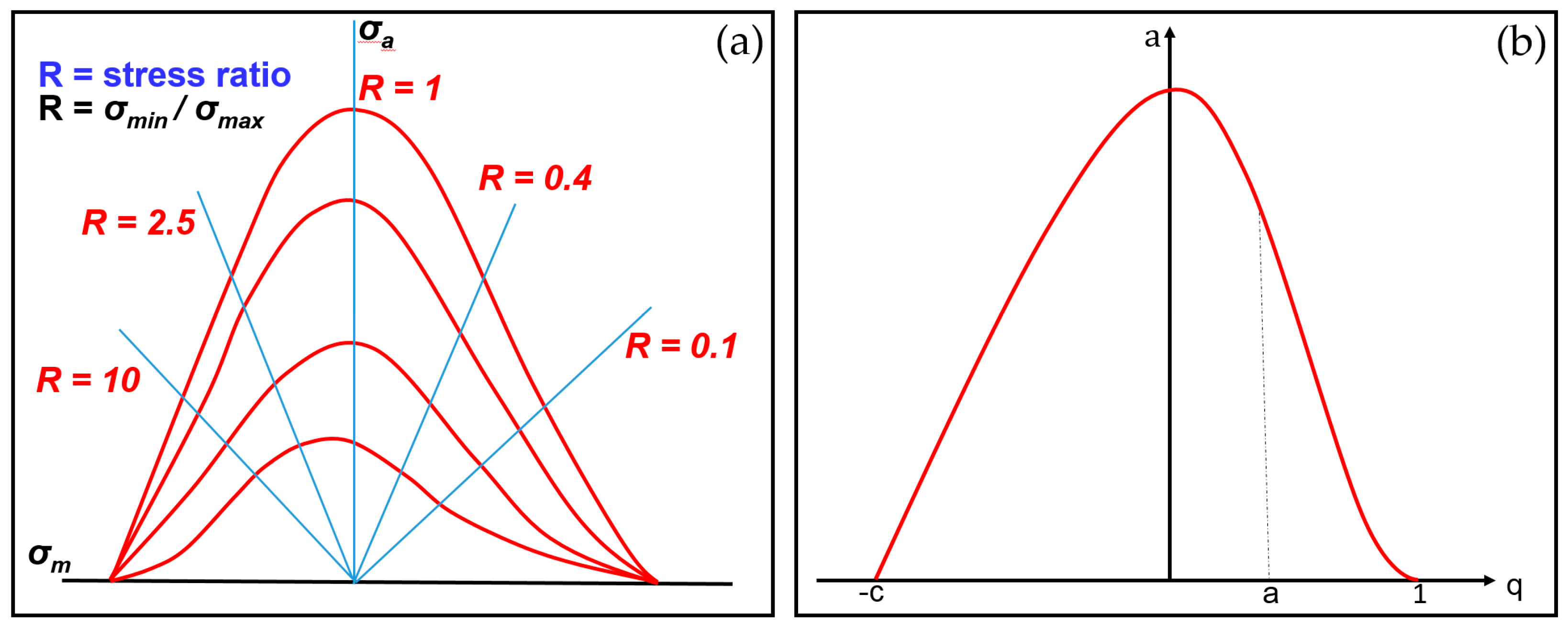
Constant life diagrams (CLD) are obtained from empirical fits to fatigue test data that relate cycles to failure to the mean and alternating stress values of the constant amplitude fatigue loading. The constant life curves are simply the contour curves corresponding to a given number of cycles of failure, plotted in the space of mean and alternating stress. Many different models and methods have been proposed to parametrically describe these curves [3]. Figure 1a shows a typical constant life diagram (CLD). The main axes on a CLD graph [20] are the mean cyclic stress () and the cyclic stress amplitude (). In addition, radial lines of constant R-ratio are shown on the graph to easily recognize how the stress ratio affects the shape of these curves. Goodman diagrams use linear fits for constant life curves. However, for composite materials researchers find that constant life curves are nonlinear and non-symmetric with respect to the mean stress axis. These curves allow interpolation of test data to estimate lifetimes for given stress loadings. A number of analytical models for parametrizing the curves have been published in literature [3,20,21,22]. Adam et al. [20] presented an analytical model that not only parametrizes the CLD but also allows unifying the different curves into a single two-parameter fatigue curve which in this work is referred to as the normalized fatigue life model (Figure 1b).
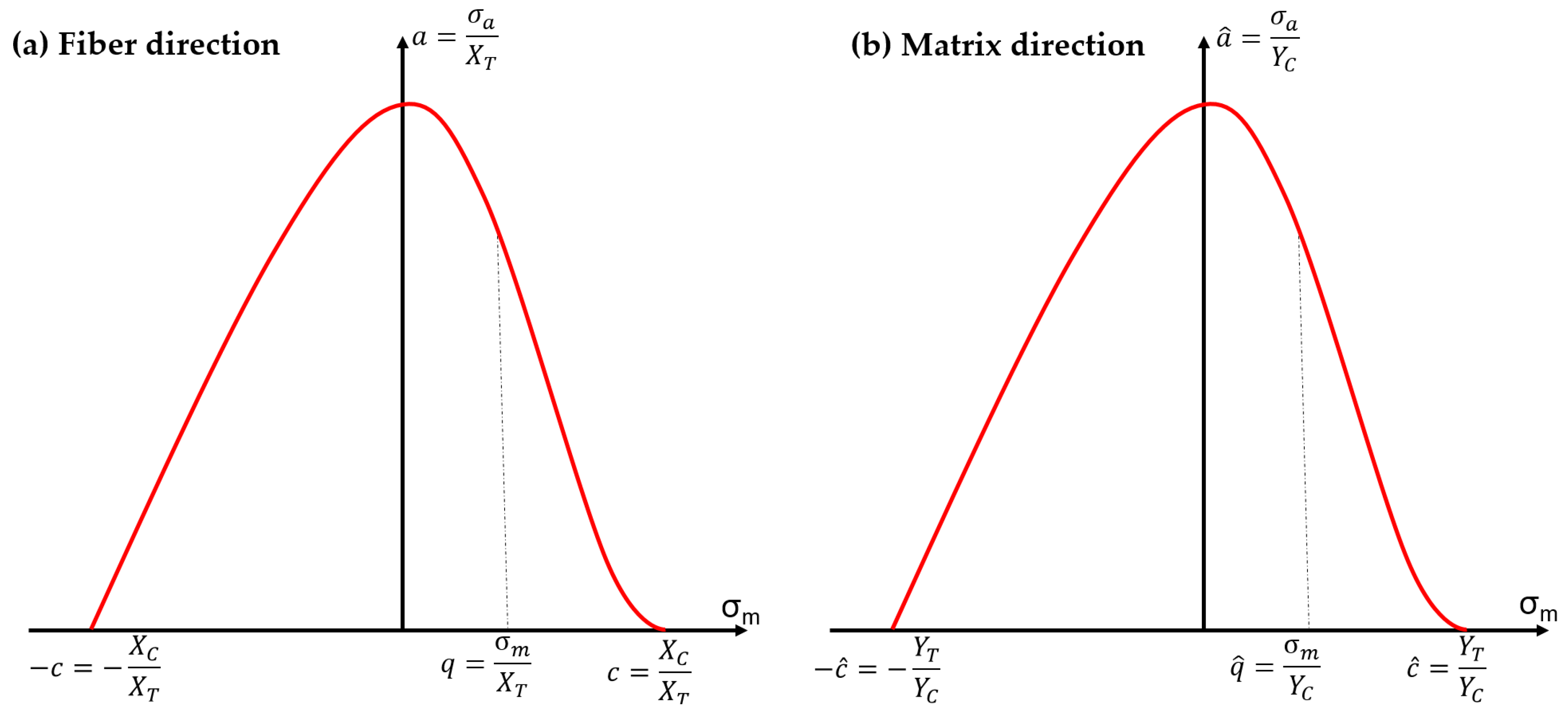
A two-parameter model of a constant life diagram was fitted to the non-dimensional mean stress q and stress amplitude a values and the ratio c of the static strengths Sref1 and Sref2 of the orthotropic ply material as shown in Equation (1).
For the composite lamina in the fiber directions, the Sref1 and Sref2 terms in Equation (1) take on values of the fiber tension and fiber compression strengths XT and XC, respectively. For the transverse to fiber direction, the Sref1 and Sref2 terms in Equation (1) take on values of the transverse to fiber compression and transverse to fiber tension strengths YC and YT, respectively. Normalization allows the definition of a unified load parameter u to fit constant life diagrams. The parametric model proposed by Adam et al. [16] is given by:
where f, u and v are model fit constants. The exponents u and v determine the shapes of the left and right wings of a bell-shaped CLD curve. However, Gathercole et al. [22] showed that the degree of curve-shape asymmetry was not very great for carbon-epoxy composites; therefore, the assumption that u and v are equal is valid. Thus, u is given by:
In Equation (3), f is a curve fitting parameter with a value of 1.06.
The unified load parameter u is used to relate the loading to the number of cycles to failure in the empirical model. Shokrieh used a linear fit model to the logarithm of the number for cycles to failure log(Nf) as a function of the unified load parameter u,
where A and B are the curve fitting constants.
The number of cycles to failure () is computed for the state of axial fiber direction loading using stress σ11 and for the transverse to fiber direction loading using stress σ22 by choosing the appropriate normalization stress in the definition of the load parameter u, as described above. Shokrieh and Lessard also showed that the unified load parameter for the pure shear state of stress (σ12, σ13, or σ23) requires modification. There is no equivalent loading direction strength tension or compression when loaded in shear. The unified load parameter for shear loading as proposed by Shokrieh [6] is
In the above expression z = σa/σshear and q = σshear/S, where σa is the stress amplitude, σshear is the applied shear stress and S is the static shear strength.
The unified parameter u, in Equation (3) is also modified slightly for loading in the transverse to fiber direction (matrix failure dominated state of stress), σ22. Our implementation of the model found that the estimation of the number of cycles to the failure using the general form of Equation (3) used by Shokrieh [6] does not provides a realistic prediction for the loading transverse to the fiber. The model is required to be normalized by the compression strength, where the general form of Equation (3) normalized using the tensile strength in the matrix direction. Implementations of Shokrieh’s model by other authors found in the literature does not address this normalization approach for the unified load parameter in the matrix direction [23,24,25,26]. The unified parameter in the state of stress σ22 is normalized by the strength parameter YC and the unified parameter, can be expressed as:
The experimental value of the transverse compressive strength YC is significantly higher than the tensile strength YT, where the longitudinal tensile strength XT is generally larger than the compressive strength XC. Therefore, for the σ22 state of stress, the normalization was performed by the compressive strength of YC, as shown in Figure 2b.
Table 1 shows a comparison of the computed values of the unified load parameters, u and using the model presented by Shokrieh [6] given Equation (5) and the modification that was made in this paper which is given by Equation (6). The accurate prediction of the unified parameter, u modification is significant to predict fatigue life along the matrix direction as failure generally initiates in the matrix.
3. Shokrieh’s Material Degradation
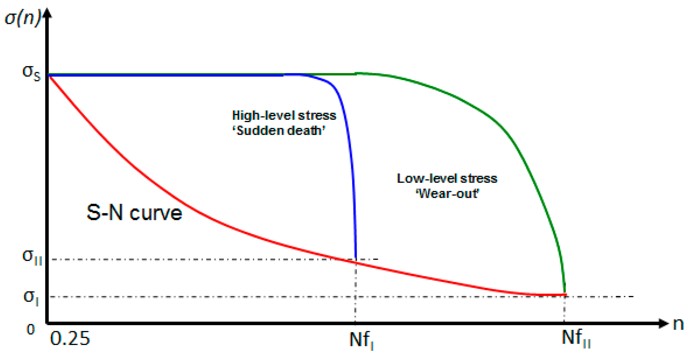
Shokrieh and Lessard [17,18] proposed a power law model (Figure 3) to represent the relationship between the number of cycles and the residual strength or stiffness of a laminate. This model is capable of capturing both the “sudden death” [27] and “wear out” [28] modes for failure in laminates. The “sudden death” mode is observed in fatigue tests at high stress levels whereas the “wear out” mode is observed in fatigue tests at low stress levels.
The power law fit for the degradation of the strength and the stiffness follows the form:
The number of cycles to failure is normalized as follows:
The residual strength and stiffness are normalized using:
Thus, the residual strength and stiffness as a function of the number of cycles, stress level and stress ratio are given by:
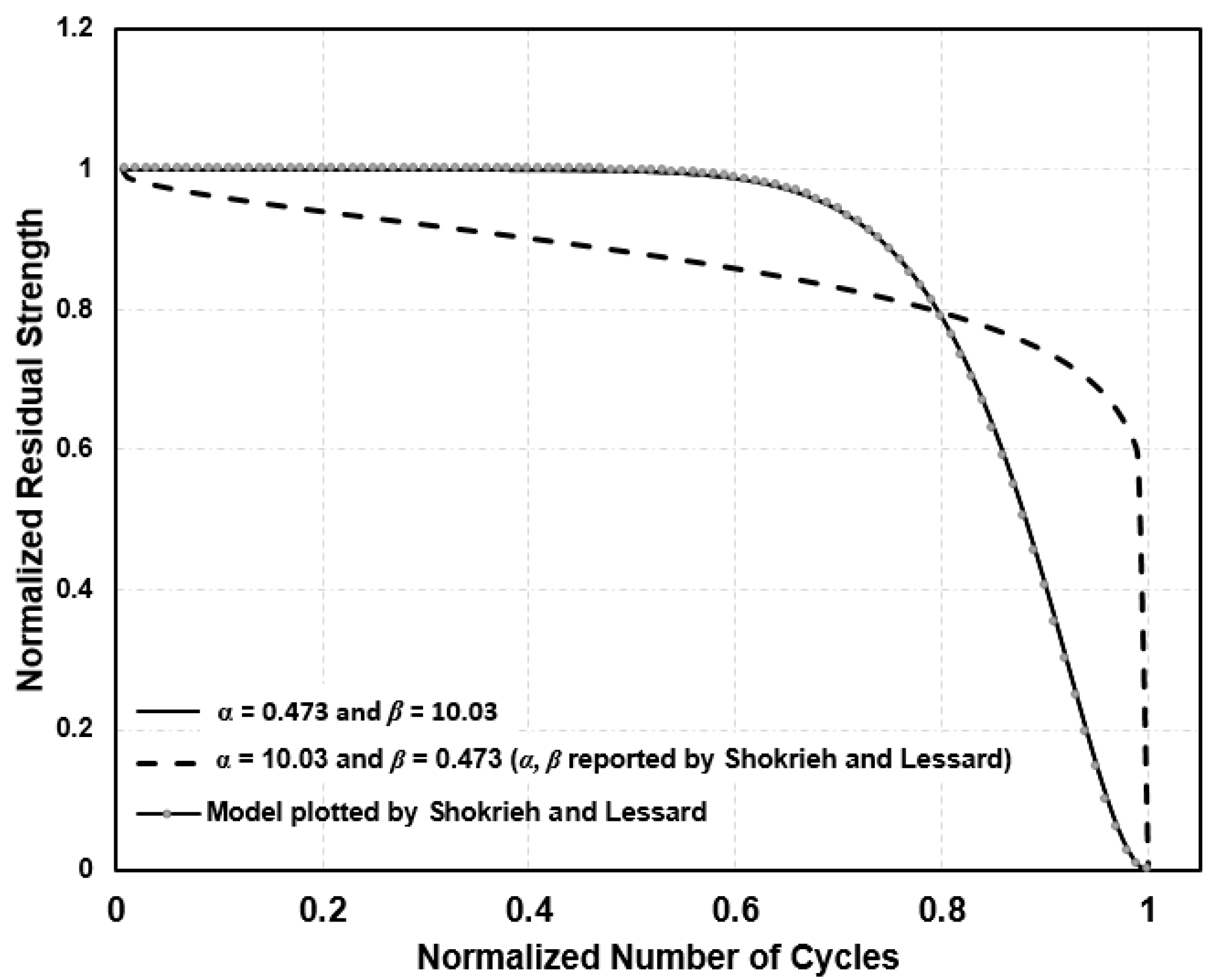
where σr is the residual strength, σ0 is static strength, σ is the stress level, n is the number of applied cycles, Nf is the number of cycles to failure at the current stress level (fatigue life), α and β are the experimental curve fitting parameters, E is the residual stiffness, σ is the stress level, n is the number of applied cycles, ES is the initial stiffness, εf is the strain at failure at applied stress σ and γ and λ are the experimental curve fitting parameters [17,18]. The curve fitting parameters α, β, γ and λ are given in Table 2. These fitting parameters provided by Shokrieh and Lessard [6,17,18,19] contain typographical errors where the α and β parameters are switched.
The material constants determined for the residual strength and the stiffness model reported by Shokrieh and Lessard contains typographical error in all the reported publications by the authors. Figure 4 shows the use of the parameters α and β for the strength degradation model of the uniaxial 0° test specimen as given by Equation (10). It is evident that the values of the parameters are switched [17,18] and causes significant discrepancies in residual strength prediction.
Cumulative Damage Approach
Number of authors have implemented Shokrieh and Lessards’s empirical model to predict fatigue behavior of composites [23,24,25,26]. The authors [23,24,25,26] did not account for any damage accumulation when the state of stress redistributes due to failure in a material point. The above models were developed using constant amplitude tests. To apply them to structural fatigue simulations under varying loads, a cumulative damage approach [29] is needed. Variations in stress amplitudes for applied stress may be due either to the applied load being time varying or to stress distributions arising from stiffness changes caused by stiffness degradation or local material failure. The cumulative damage approach introduces a damage variable to track damage accumulations and maintains continuity of the damage variable when stress changes occur. In this way damage accumulation at a new stress level starts with the initial damage level being what was sustained already due to previous history at different stress levels. The cumulative damage not only account for the damage due to the stress state redistribution but also accounts for the existing damage.
If a material that degrades due to cyclic loading is subjected to uniaxial fatigue load with maximum stress σ, failure occurs when the residual strength σr, reaches the applied stress level σ. Using the strength degradation model (Equation (10)), the ratio of the stress margin due to the degradation of strength after n cycles, to the maximum stress margin at start of the fatigue loading is expressed as:
where σr, is the residual strength, (n) is the number of cycles at applied load and (Nf) is the number of cycles to failure. The above ratio varies from unity at start to zero at failure. In this work, we adopt a definition of damage based on the reduction in material strength. The damage variable D therefore takes the form:
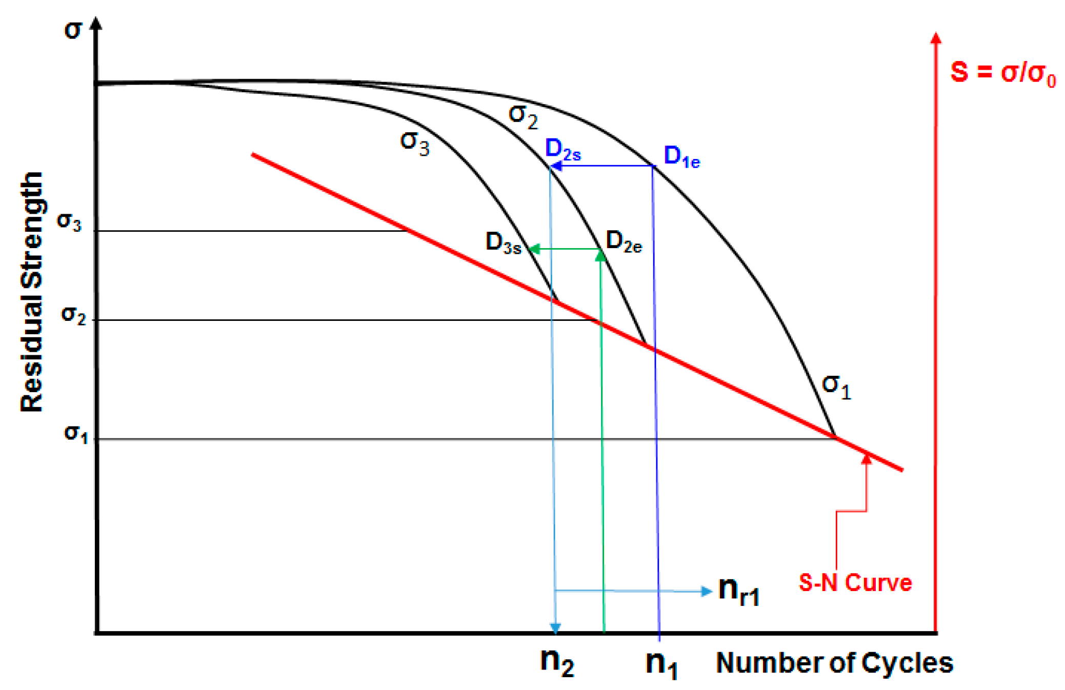
Figure 5 provides a schematic of the cumulative damage approach. The curves represent the residual strength degradation as a function of the number of cycles for different constant amplitude fatigue loading stress levels . Connecting the end points of each curve also gives the S-N curve. In the cumulative damage approach, we maintain equivalency of damage between fatigue cycles when there is a stress level change by equating the residual strength. Let us assume D1e is the damage accumulated at the end of the elapsed loading block of n1 fatigue cycles at stress level σ1. If the stress level changes to σ2 after the first block of n1 fatigue cycles at stress level σ1, the damage accumulation starts of the new block D2s must be equal to D1e. To use a degradation model for constant amplitude loading, with the new stress level σ2 we calculate first the equivalent number of cycles of loading at stress level σ2 that would have created the damage level D1e. Using the definition of damage in Equation (13), the equivalent cycles is calculated as shown below in Equation (14).
The remaining life at stress level σ2 is . If this is greater than zero then the fatigue loading can continue and the material degrades following the degradation law corresponding to stress level σ2. The damage accumulation in the new block n2 cycles at stress level σ2 is calculated based on total cycle count equal to . For any kth new block of fatigue load, we calculate the equivalent elapsed cycles as and the remaining life using Equation (15).
4. Failure Criteria and Instant Material Degradation
In our work, we use Hashin’s [30] failure criteria to determine the fiber and matrix failures in a unidirectional lamina. Equations (16)–(19) summarize equation for the failure envelopes for fiber and matrix failure from Hashin’s criteria.
Fiber failure in tension
Fiber failure in compression
Matrix failure in tension (σ22 + σ33 ≥ 0)
Matrix failure in compression (σ22 + σ33 < 0)
In Equations (16)–(19), XT and XC are the longitudinal tensile and compressive strengths, YT and YC are the transverse tensile and compressive strengths, S12 is the in-plane shear strength and S23 is the out of plane shear strength. An instantaneous ply stiffness degradation scheme is used for the progressive failure when ply failure is detected. Camanho [31] showed that a small but finite residual stiffness after failure is needed to accurately predict the evolution of progressive failure. Table 3 shows the residual stiffness of the ply following failure in each mode.
5. Finite Element Implementation
Finite element analysis software ABAQUS [32] was used to perform the fatigue analysis of composite laminates and laminates structures. Fatigue material degradation was implemented as a user-defined material subroutine (UMAT) for use in ABAQUS non-linear implicit solution. The laminates were modelled as a three-dimensional solid with ply by ply representation. Each ply was modeled using the eight-node bilinear reduced integration C3D8R solid elements, with enhanced hourglass control. Figure 6 shows a flow chart of the material degradation model implementation. The Jacobian update implemented in the UMAT subroutine was consistent for use with geometric nonlinear analyses. Failure indices, residual strengths and damage parameters at each integration point are stored as Solution Dependent Variables (SDVs) in ABAQUS.
The fatigue loading is simulated by two load steps: a static load step under load control up to the maximum loading during each cycle, followed by a constant load over a specified time. The degradation with cycles is performed with a forward time marching scheme in with an increment of 1000 cycles for each time increment in the second step. To determine residual stiffness, additional load steps are added to unload the structure and then load the structure under displacement control until failure.
6. Verification and Validation
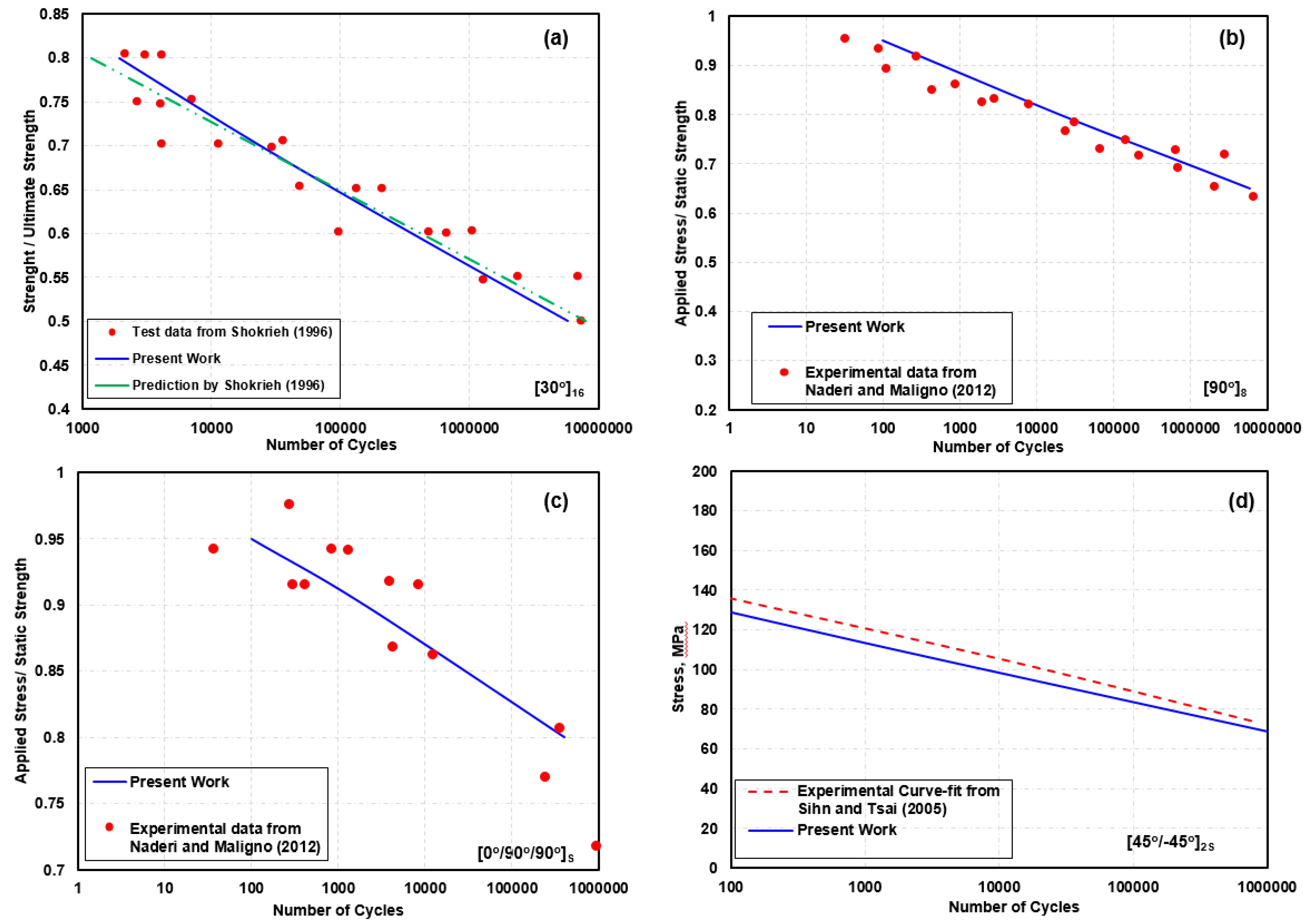
The UMAT subroutine implemented in ABAQUS was first verified using experimental data for the six unidirectional laminate cases presented by other authors for stress ratios of R = 0.1 and 10. This was followed by simulations of laminate coupons tested under homogenous stress states. Figure 7 shows the comparison of the model predicted S-N curve with experimental data and simulations results obtained from the literature for [30°]16 laminate from Ref. [6], [90°]8 laminate from Ref. [23], [0°/90°/90°]S from Ref. [23] and [45°/−45°]2s from Ref. [33]. The test data exhibits significant scatter. The empirical model predictions lie within the scatter of the test data, except for the fatigue test at loading level at 80% of ultimate strength. All tests and simulations correspond to AS4/3501-6 graphite epoxy composite from Shokrieh and Lessard [6] and listed in Table 2 and Table 4.
7. Open-Hole Tension Specimen
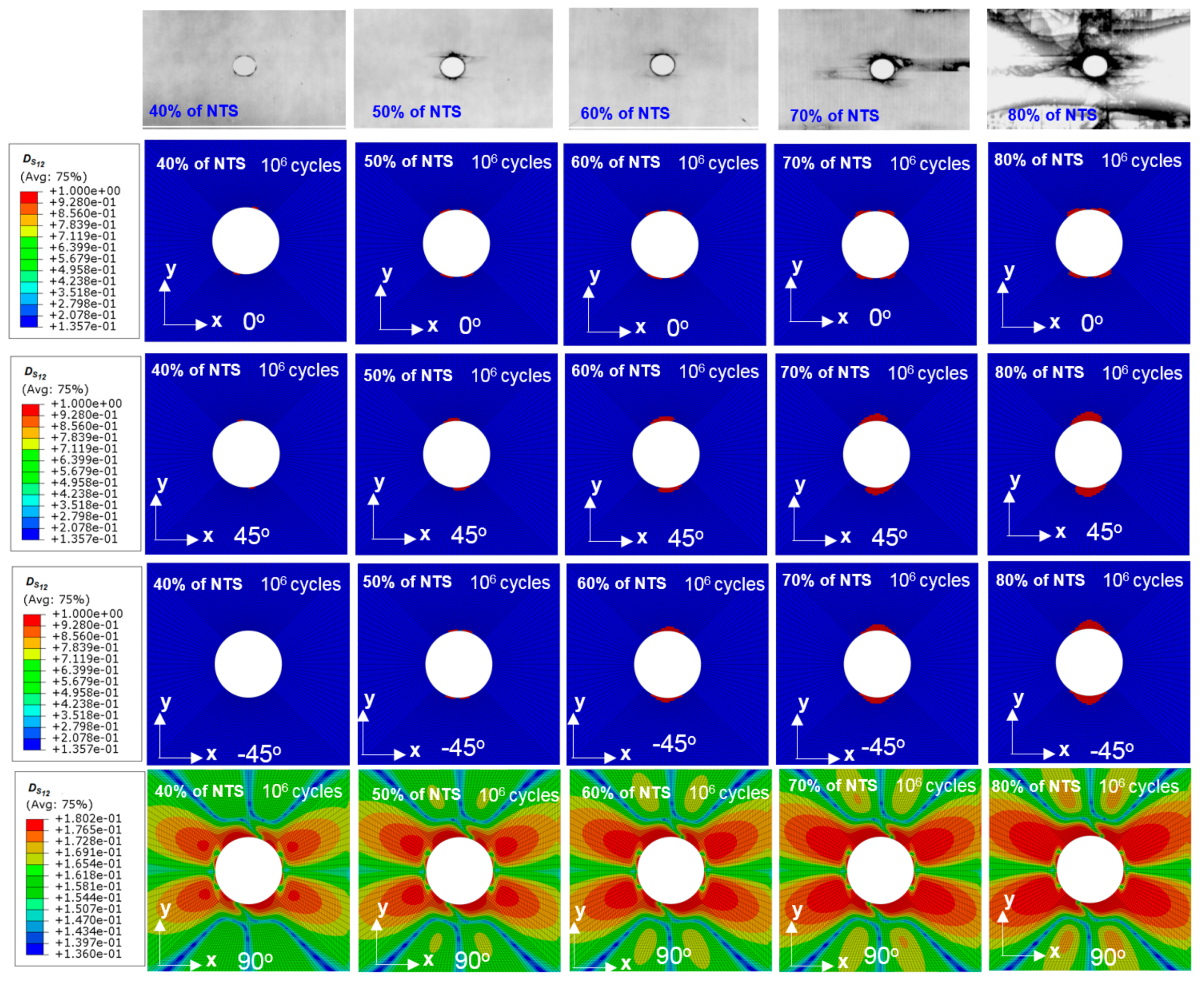
Han et al. [34] published experimental data for open-hole specimen fatigue tests performed for AS4 3501-6 composite material laminates. They tested seventy open-hole-laminate coupon specimens under constant amplitude tension and compression fatigue loading. The laminate tested was a 24-ply quasi-isotropic [0/ ± 45/90]3S laminate. The tension-tension fatigue tests at R = 0.1 were performed for maximum stress levels of 40%, 50%, 60%, 70% and 80% of the Notched Tensile Strength (NTS) of the laminate. NTS is the ultimate stress at failure of the laminate under quasi-static tension loading. After one million fatigue cycles at 40%, 50%, 60%, 70% and 80% of the NTS, the specimens were loaded to static failure to obtain the Residual Tensile Strength (RTS).
The instantaneous degradation scheme is known to be mesh sensitive. In fatigue only a small region around the hole sustains damage due to the stress concentration. However, to perform progressive failure to get NTS or RTS, where damage leads to two part failure of the specimen, the entire width of the specimen at the hole was finely meshed. The region away from the damage region where the mesh was not refined was modeled as elastic and did not include the UMAT provided damage degradation. This resulted in a mesh with total 13,600 elements in each ply and 11,600 elements in the refined mesh region (Figure 8).
Figure 9 shows the stress strain response of the laminate under quasi-static loading in pristine state and post fatigue tested state. The inset shows the ungripped portion of the specimen model for FE simulations. Table 5 summarizes the comparisons of the predicted and experimental values of NTS and RTS of the notched laminate specimen.
The experimentally measured NTS of the specimen [34] was 413 MPa. Progressive failure analysis prediction of NTS using the Hashin’s failure criteria and instantaneous stiffness degradation describer earlier was 405 MPa. It is to be noted the material properties for AS4 3501-6 used for analyses were from Shokrieh [6] as this was not provided in the reports of Han et al. [34]. No material property calibrations were done to match test results. Progressive failure analysis of the pristine specimen shows that the specimen experiences matrix damage in the 90° and ±45° plies at 40% of the NTS. This means for fatigue loading above this level there is damage from the very first cycle. This damage is higher when the specimen is loaded at 50 to 80% of the NTS. Fatigue damage for these cases represents growth of the initial damage.
The prediction the fatigue residual strength RTS notched specimens subjected to constant amplitude cyclic loading at 40%, 50%, 60% and 70% for 106 cycles, showed an increase in the residual strength. The local damage around the hole leads to stress distributions that minimize the stress concentration at the hole. The slope of the axial stress–strain curve (Figure 9) from progressive failure analyses of the specimens in post-fatigued state with simulated fatigue damage shows that the damage leads to a relatively small stiffness loss for cases when the fatigue loading maximum stress levels were 40% to the 70% of NTS. This is due to the fatigue damage being primarily due to matrix failure and damages being localized to the region around the hole. The stiffness loss due to fatigue damage was 12% for the specimen loaded at 80% of the NTS. None of the specimens failed after one million fatigue cycles at stress levels 40–80% of NTS. Post inspection of the tested specimens tested at 80% of the NTS showed significant delamination and edge peeling of the plies [34]. The delamination fatigue damage mode is not included in our fatigue analysis model.
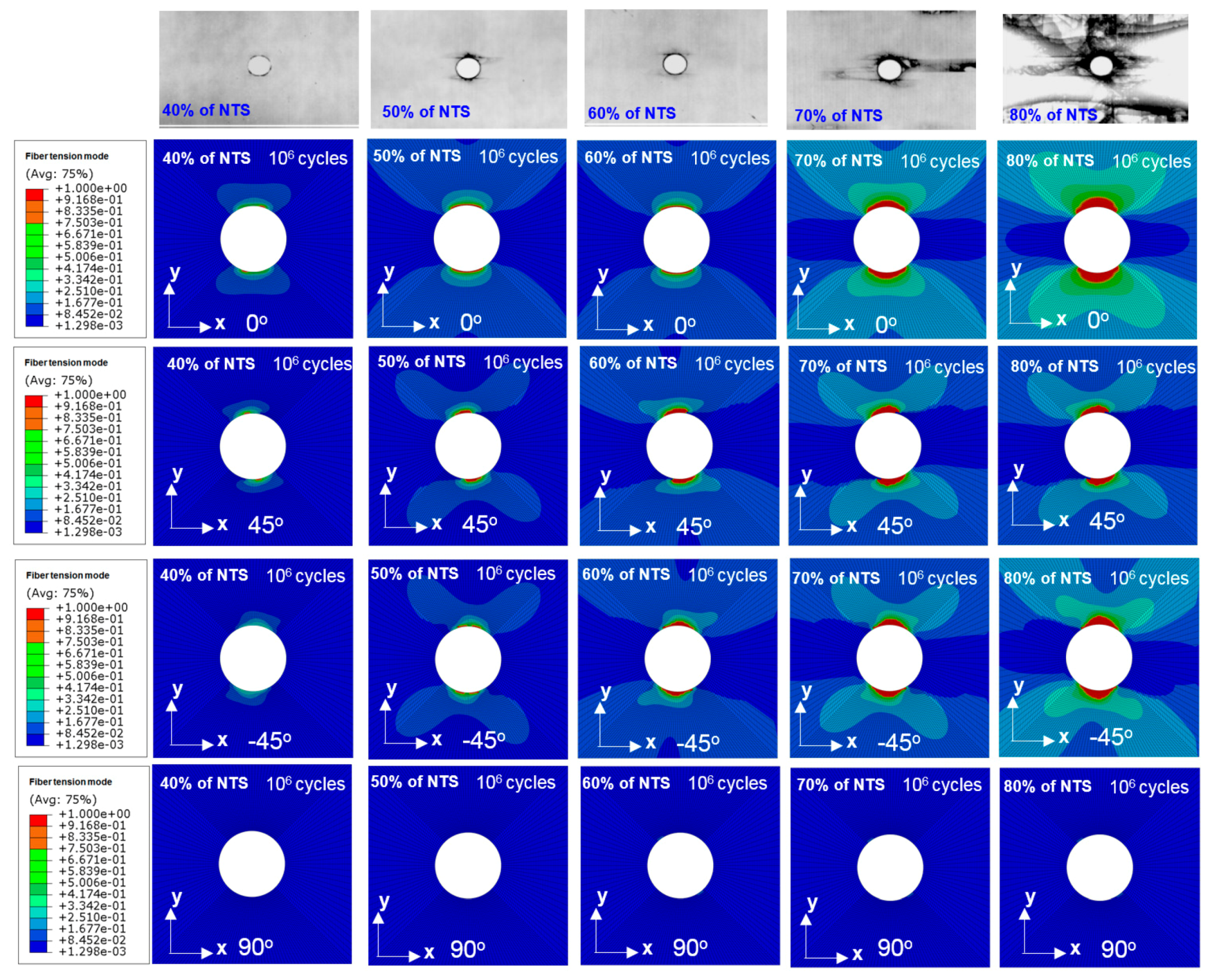
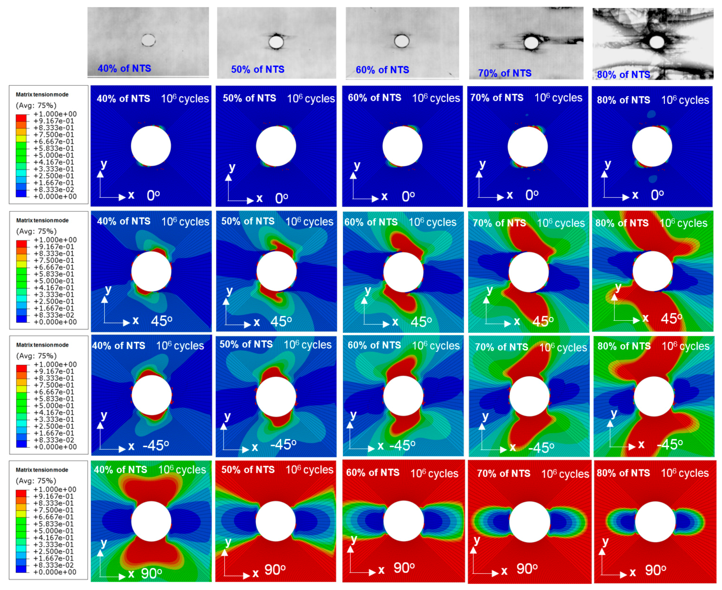
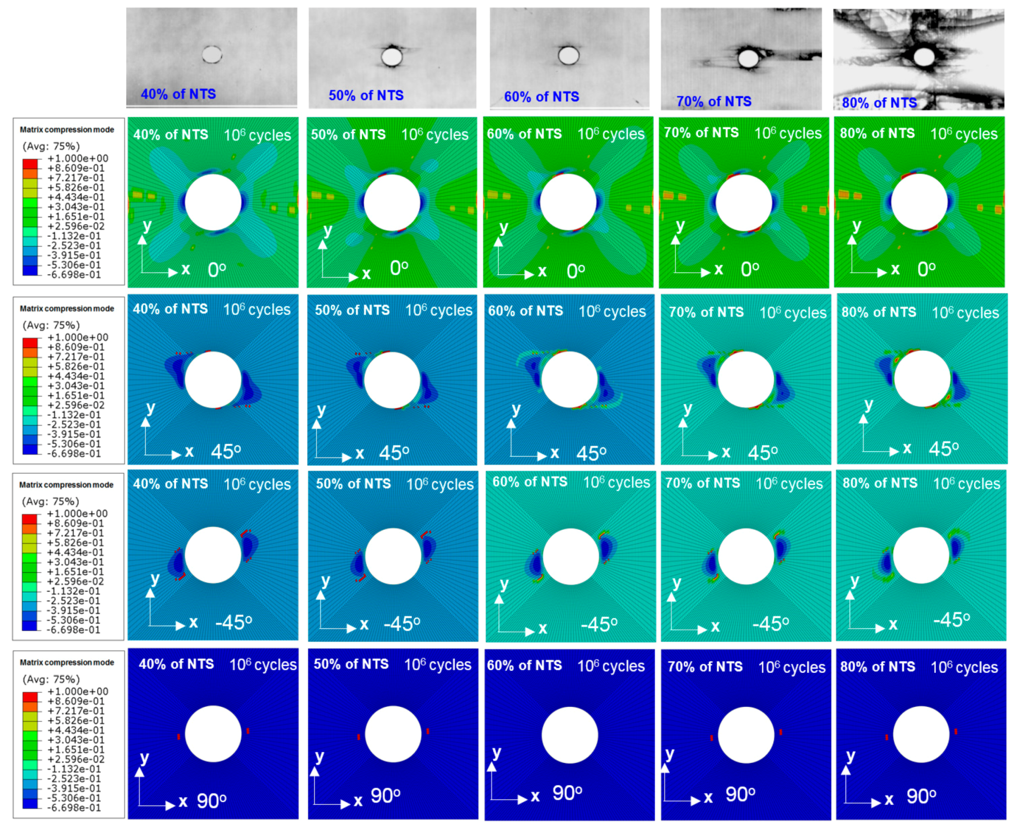
During a fatigue loading simulation, as the strength degrades the failure index increases until it reaches the critical value of one, at which point the ply is considered to be fully failed. Figure 10, Figure 11, Figure 12 and Figure 13 show contour plots of the failure indices in each ply for all four failure modes after one million fatigue cycles at 40–80% of the NTS. Failed elements are indicated by failure index of 1.0. The contour plots of the failure indices show the extent of failure and the margin to failure at the maximum stress level of the fatigue load cycle. Examination of these failure indices indicate that there is significant fatigue damage in matrix tension mode in 45° and 90° plies and matrix compression mode in the 0° plies and some fatigue damage due to fiber tension mode in the 0° plies at the edge of the hole.
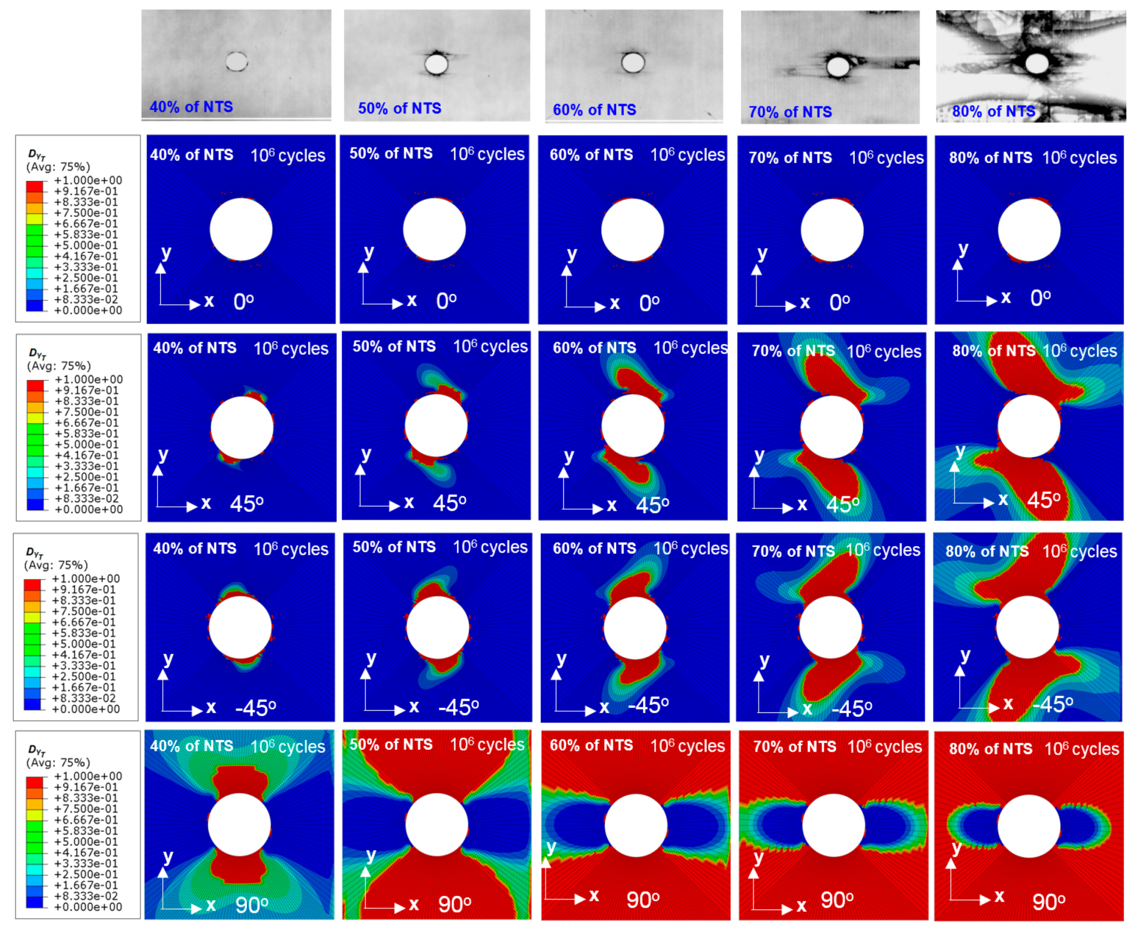
The fatigue model used here is based on stiffness and strength reduction directly applied to the engineering stiffness constants and strengths that are ply properties. To quantify and visualize the level of damage, a measure of the relative reduction in the stiffness/strength parameter due to damage , is calculated using Equation (20).
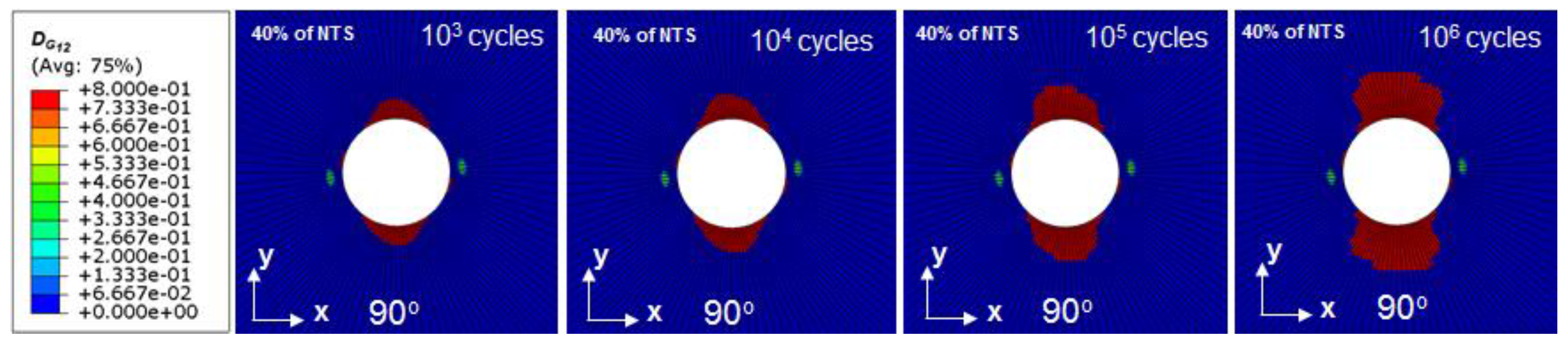
Figure 14, Figure 15, Figure 16, Figure 17 and Figure 18 show the relative reduction of stiffness and strength properties due to fatigue damage that exceeded 10%. The significant reductions (80–100%) are observed in the transverse to fiber (matrix) direction moduli E2 and tension strength YT and the plane shear moduli G12 in the 90° ply along the symmetry plane perpendicular to the loading direction. A small (less than 20%) reduction in in-plane shear strength is observed in all plies. Although the laminate is loaded in its plane, reduction of in-plane properties leads to transverse shear stresses (captured by the 3D modeling) that induce damage and reduction in transverse shear strengths S23. Although none of the specimen experienced complete failure under tension-tension loading after a million cycles, radiograph images show significant damage. The Figure 14, Figure 15, Figure 16, Figure 17 and Figure 18 show the X-ray radiograph images of the damage accumulated in the specimen from Han et al. [34] at load level of 40–80% of the NTS. Significant damage is visible at 50%, 60% and 70% of NTS, even though the change in residual strength is not significantly high. At 80% of the NTS the damage state is significantly visible in the specimen as several modes of failure can cause the damage. In addition to the matrix damage the specimen also experienced delamination mode of failure.
Figure 19 and Figure 20 show the evolution of damage quantified by the relative reductions in the transverse tensile strength and in-plane shear stiffness of the ply. The progression shows that the damage starts early (103 cycles) and continues to grow in a stable fashion. It is to be noted that while stiffness degradations redistribute loads to other plies leading to small decreases in stress. This has the potential to arrest the progression damage. The degradation in matrix properties do not seem to play a significant role on the overall stiffness or strength of the notched specimen. This is because the transverse (matrix) stiffness is one order of magnitude lower than fiber direction stiffness in our laminate. However, quantifying matrix damage is useful as matrix damage is undesirable as it can lead to delamination. The matrix damage also makes the composite prone to moisture intrusion or leakage.
The effect of the interlaminar failure and damage patterns are shown by researchers for open hole composite specimens under tensile loading. Archard et al. [35] presented a discrete ply model approach to experimentally quantify damage under static loading for a composite plate with a hole under tensile loading. Nixon-Pearson et al. [36] presented an extensive experimental framework to show the sequence of damage development throughout the life of open-hole quasi-isotropic IM7/8552 carbon fiber/epoxy laminates loaded in tension–tension fatigue. Work of Nixon-Pearson et al. [36] showed that there is delamination between 0/45 and 45/90 layers during fatigue cycles. For the open hole tension specimen, we have depicted the reduction in the strength and stiffness properties in each ply and determined the residual strength of the specimen after a million fatigue cycles. The ultimate strength was determined using Hashin’s failure criteria where right after fiber failure the stiffness E1 was reduced to 7% of its initial value (Table 3). Thus, the effect of delamination to predict the ultimate residual strength of the specimen can be neglected mostly due the nature of the intralaminar failure of the specimen for predicting residual strength.
The methodology presented in this paper was specific to the model and material parameters presented by Shokrieh and Lessard [17,18]. The primary goal of this paper was to develop and present a FE framework by using a UMAT subroutine to predict residual strength of the open hole specimen and show intralaminar damage plots in each ply. The number of parameters associated with the model can be significant sources of uncertainty. The model contains forty two parameters that is required to be calibrated from unidirectional tests. Thus, a separate study for the uncertainty quantification is required for the model. Using high fidelity model such as a continuum damage mechanics (CDM) based model has shown that fewer number of such fatigue parameters [37]. The methodology (FE framework) can be extrapolated to any sets of material provided the material parameters (Table 2) for static and fatigue tests are available from experiment.
Shokrieh’s [6,16,17] model develops the empirical S-N curves, stiffness and strength degradation using uniaxial tests along each material direction and uses these models for multiaxial fatigue. However, the model has some limitations. The model does not capture the correlation or interaction between the degradation in stiffness and the residual strength parameters along different material directions of the ply. Matrix cracking failure should cause degradation of both the transverse normal and shear properties. In this model, the transverse to fiber property degradation is only due to transverse stress and the in-plane shear property degradation is only due to shear loads. The matrix cracking failures in the plies is induced by both transverse to fiber normal stresses and shear stresses. The model can be improved fitting the empirical models to the evolution of damage variables with these damage variables used to compute the constitutive stiffness and strength properties following a continuum damage approach. The models used for fatigue analysis of composites can be categorized by the fidelity of the model. In most of the cases empirical models are considered as lower fidelity model with less computational time but often having large number of fatigue parameters. Higher fidelity model includes the Continuum Damage Mechanics based model and micro-mechanics based models that are computationally expensive. Computationally cheap lower fidelity models can significantly aid in multi-level and multifidelity modeling approaches for uncertainty quantification [38]. Our revisit of the Shokrieh and Lessard model [17,18] was for its use as a low fidelity model in a multifidelity framework. However, the inherent typographical errors in the original publication and ensuing citations to the paper led to large discrepancies. In this paper, we present the corrected version for these fit parameters reported by Shokrieh and Lessard [17,18]. As a result of the corrections the low fidelity model provides an improved prediction accuracy that can be further refined and calibrated with other high fidelity models.
8. Conclusions
This paper presents the empirical stiffness and strength degradation model of Shokrieh’s [6], its implementation as a user material subroutine UMAT in ABAQUS FE software and its validation using test data from literature. The results indicate this empirical model can provide a good engineering estimate of fatigue life and residual strength for preliminary design analysis. The modification in the definition of the unified load parameter for the transverse to the fiber direction improved the prediction accuracy.
We found that residual strength for open-hole tension specimen is mostly related to fatigue failure in the fiber failure in 0 degree plies. Our developed user defined material subroutine (UMAT) enabled us to predict residual strength of the open hole tension specimen without the inclusion of any delamination model. The translaminar failure is captured by the degradation of the transverse normal and shear moduli of the lamina. The inclusion of the cumulative damage model adds to the capabilities to account for the stress level changes due to the failure during fatigue loading.
FE based progressive failure analysis with instantaneous degradation is highly mesh size sensitive and requires mesh convergence studies. In uncertainty quantification, the discretization errors must therefore be included as a source of model uncertainty. Further, the value of the residual stiffness used after ply failure has a significant influence on the peak load. For example, changing the residual stiffness from the values listed in Table 1 to a uniform 4% value reduces the NTS and RTS values by 25%. The lack of correlation between degradations to transverse to fiber direction normal modulus and in plane shear due to matrix damage is also a source of model error. These two are the most significant source of epistemic uncertainty that needs higher fidelity models and test data to correct.
Acknowledgments
This work was performed under a contract from the Air Force Office of Scientific Research FA8650-16-C-5010-01.
Author Contributions
Arafat I. Khan and Satchi Venkataraman contributed to the model implementation and contributed in writing the paper. Ian Miller contributed to discussions during the implementation and provided valuable suggestions to the work reported here.
Conflicts of Interest
The authors declare no conflict of interest.
References
- Degrieck, J.; Van Paepegem, W. Fatigue damage modeling of fiber-reinforced composite materials: Review. Appl. Mech. Rev. 2001, 54, 279–300. [Google Scholar] [CrossRef]
- Hashin, Z.; Rotem, A. A fatigue failure criterion for fiber reinforced materials. J. Compos. Mater. 1973, 4, 448–464. [Google Scholar] [CrossRef]
- Vassilopoulos, A.P.; Mashie, B.D.; Keller, T. Influence of the constant life diagram formulation on the fatigue life prediction of composite materials. Int. J. Fatigue 2010, 324, 659–669. [Google Scholar] [CrossRef]
- Whitworth, H.A. A stiffness degradation model for composite laminates under fatigue loading. Compos. Struct. 1997, 40, 95–101. [Google Scholar] [CrossRef]
- Zhang, Y.; Vassilopoulos, A.P.; Keller, T. Stiffness degradation and fatigue life prediction of adhesively-bonded joints for fiber-reinforced polymer composites. Int. J. Fatigue 2008, 30, 1813–1820. [Google Scholar] [CrossRef]
- Shokrieh, M. Progressive Fatigue Damage Modeling of Composite Materials. Ph.D. Thesis, McGill University, Montreal, QC, Canada, 1996. [Google Scholar]
- Philippidis, T.P.; Passipoularidis, V.A. Residual strength after fatigue in composites: Theory vs. experiment. Int. J. Fatigue 2007, 29, 2104–2116. [Google Scholar] [CrossRef]
- Mao, H.; Mahadevan, S. Fatigue damage modelling of composite materials. Compos. Struct. 2002, 58, 405–410. [Google Scholar] [CrossRef]
- Van Paepegem, W. Development and Finite Element Implementation of a Damage Model for Fatigue of Fibre-Reinforced Polymers. Ph.D. Thesis, Ghent University, Ghent, Belgium, 2002. [Google Scholar]
- Krüger, H.; Rolfes, R. A physically based fatigue damage model for fibre-reinforced plastics under plane loading. Int. J. Fatigue 2015, 70, 241–251. [Google Scholar] [CrossRef]
- Reifsnider, K.L.; Stinchcomb, W.W. A critical-element model of the residual strength and life of fatigue-loaded composite coupons. In Composite Materials: Fatigue and Fracture; ASTM STP 907; Han, T., Ed.; ASTM International: Washington, DC, USA, 1986; pp. 298–313. [Google Scholar]
- Pineda, E.J.; Bednarcyk, B.A.; Arnold, S.M. Validated progressive damage analysis of simple polymer matrix composite laminates exhibiting matrix microdamage: Comparing macromechanics and micromechanics. Compos. Sci. Technol. 2016, 133, 184–191. [Google Scholar] [CrossRef]
- Chiachío, M.; Chiachío, J.; Rus, G.; Beck, J.L. Predicting fatigue damage in composites: A Bayesian framework. Struct. Saf. 2014, 51, 57–68. [Google Scholar] [CrossRef]
- Chiachío, J.; Chiachío, M.; Saxena, A.; Sankararaman, S.; Rus, G.; Goebel, K. Bayesian model selection and parameter estimation for fatigue damage progression models in composites. Int. J. Fatigue 2015, 70, 361–373. [Google Scholar] [CrossRef]
- Sankararaman, S.; Ling, Y.; Mahadevan, S. Uncertainty quantification and model validation of fatigue crack growth prediction. Eng. Fract. Mech. 2011, 78, 1487–1504. [Google Scholar] [CrossRef]
- Diao, X.; Lessard, L.B.; Shokrieh, M.M. Statistical model for multiaxial fatigue behavior of unidirectional plies. Compos. Sci. Technol. 1999, 59, 2025–2035. [Google Scholar] [CrossRef]
- Shokrieh, M.M.; Lessard, L.B. Multiaxial fatigue behavior of unidirectional plies based on uniaxial fatigue experiments-I. Modelling. Int. J. Fatigue 1997, 19, 201–207. [Google Scholar] [CrossRef]
- Shokrieh, M.M.; Lessard, L.B. Multiaxial fatigue behavior of unidirectional plies based on uniaxial fatigue experiments-II. Experimental evaluation. Int. J. Fatigue 1997, 19, 209–217. [Google Scholar] [CrossRef]
- Shokrieh, M.M.; Zakeri, M. Generalized technique for cumulative damage modeling of composite laminates. J. Compos. Mater. 2007, 22, 2643–2656. [Google Scholar] [CrossRef]
- Adam, T.; Fernando, G.; Dickson, R.F.; Reiter, H.; Harris, B. Fatigue life prediction for hybrid composites. Int. J. Fatigue 1989, 11, 233–237. [Google Scholar] [CrossRef]
- Harris, B.; Reiter, H.; Adam, T.; Dickson, R.F.; Fernando, G. Fatigue behaviour of carbon fibre reinforced plastics. Composites 1990, 21, 232–242. [Google Scholar] [CrossRef]
- Gathercole, N.; Adam, T.; Harris, B.; Reiter, H. A Unified Model for Fatigue Life Prediction of Carbon Fibre/Resin Composites. In Developments in the Science and Technology of Composite Materials ECCM 5; Elsevier Applied Science: Bordeaux, France, 1992; pp. 89–94. [Google Scholar]
- Naderi, M.; Maligno, A.R. Fatigue life prediction of carbon/epoxy laminates by stochastic numerical simulation. Compos. Struct. 2012, 94, 1052–1059. [Google Scholar] [CrossRef]
- Naderi, M.; Maligno, A.R. Finite element simulation of fatigue life prediction in carbon/epoxy laminates. J. Compos. Mater. 2013, 47, 475–484. [Google Scholar] [CrossRef]
- Shokrieh, M.M.; Taheri-Behrooz, F. Progressive fatigue damage modeling of cross-ply laminates, I: Modeling strategy. J. Compos. Mater. 2010, 44, 1217–1231. [Google Scholar] [CrossRef]
- Shokrieh, M.M.; Taheri-Behrooz, F. A unified fatigue life model based on energy method. Compos. Struct. 2006, 75, 444–450. [Google Scholar] [CrossRef]
- Chou, P.C.; Croman, R. Residual strength in fatigue based on the strength-life equal rank assumption. J. Compos. Mater. 1978, 12, 177–194. [Google Scholar] [CrossRef]
- Halpin, J.C.; Jerina, K.L.; Johnson, T.A. Characterization of composites for the purpose of reliability evaluation. In Analysis of the Test Methods for High Modulus Fibers and Composites; ASTM STP 521; ASTM International: Washington, DC, USA, 1973; pp. 5–64. [Google Scholar]
- Hashin, Z. Cumulative damage theory for composite materials: Residual life and residual strength methods. Compos. Sci. Technol. 1985, 23, 1–19. [Google Scholar] [CrossRef]
- Hashin, Z. Failure criteria for unidirectional fiber composites. J. Appl. Mech. 1980, 47, 329–334. [Google Scholar] [CrossRef]
- Camanho, P.P.; Matthews, F.L. A progressive damage model for mechanically fastened joints in composite laminates. J. Compos. Mater. 1999, 33, 2248–2280. [Google Scholar] [CrossRef]
- Abaqus™/Standard, Users Manuals V6.14-2; Dassault Systèmes Simulia Corp.: Pawtucket, RI, USA, 2014.
- Sihn, S.; Tsai, S.W. Prediction of fatigue S-N curves of composite laminates by Super Mic–Mac. Compo. Part A 2005, 36, 1381–1388. [Google Scholar] [CrossRef]
- Han, H.T.; Choi, S.W. The Effect of Loading Parameters on Fatigue of Composite Laminates: Part V; DOT/FAA/AR-01/24; Office of Aviation Research: Washington, DC, USA, 2001.
- Achard, V.; Bouvet, C.; Castanié, B.; Chirol, C. Discrete ply modelling of open hole tensile tests. Compos. Str. 2014, 113, 369–381. [Google Scholar] [CrossRef] [Green Version]
- Nixon-Pearson, O.J.; Hallett, S.R. An investigation into the damage development and residual strengths of open-hole specimens in fatigue. Compos. A Appl. Sci. Manuf. 2015, 69, 266–278. [Google Scholar] [CrossRef]
- Khan, A.I.; Venkataraman, S.; Miller, I. Predicting Fatigue Damage of Composites Using Strength Degradation and Cumulative Damage Model. In Proceedings of the SciTech 2018—AIAA Science and Technology Forum, Kissimmee, FL, USA, 8–12 January 2018. [Google Scholar]
- Eldred, M.S.; Geraci, G.; Gorodetsky, A.; Jakeman, J. Multilevel-Multidelity Approaches for Forward UQ in the DARPA SEQUOIA Project. In Proceedings of the SciTech 2018—AIAA Science and Technology Forum, Kissimmee, FL, USA, 8–12 January 2018. [Google Scholar]
Figure 1.
(a) Schematic of a typical constant life diagram; (b) Normalized fatigue life model derived from constant life diagram.
Figure 1.
(a) Schematic of a typical constant life diagram; (b) Normalized fatigue life model derived from constant life diagram.

Figure 2.
Unified parameter determination for (a) fiber direction; (b) matrix direction loading.

Figure 3.
The sudden death and wear out model for the power law fit used in Shokrieh’s model.

Figure 4.
The normalized residual strength model for the 0° specimen tested by Shokrieh and Lessard showing the effect of the parameters α and β obtained from the test data.
Figure 4.
The normalized residual strength model for the 0° specimen tested by Shokrieh and Lessard showing the effect of the parameters α and β obtained from the test data.

Figure 5.
A schematic showing the cumulative damage approach.

Figure 6.
Flow chart of the FEM implementation using UMAT subroutine.
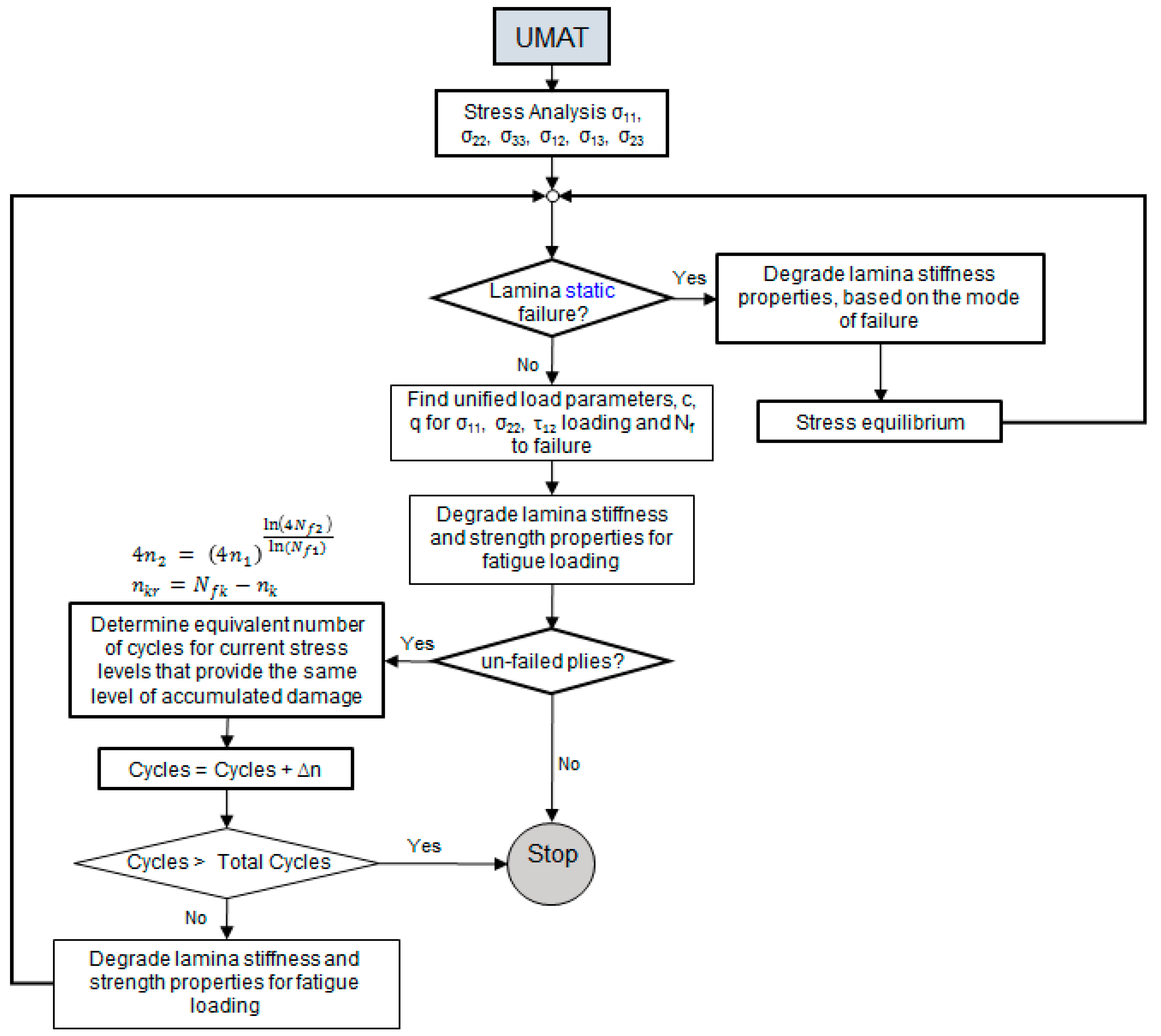
Figure 7.
Comparison of fatigue life of present numerical modeling and available experimental data for AS4/3501 laminate subjected to tension–tension fatigue loading at the frequency of 10 Hz and 0.1 load ratio. (a) [30°]16 laminate from Ref. [6]; (b) [90°]8 laminate from Ref. [23]; (c) [0°/90°/90°]S from Ref. [23] and (d) [45°/−45°]2s from Ref. [33].

Figure 8.
Mesh used for the notched tensile test specimen analyses.
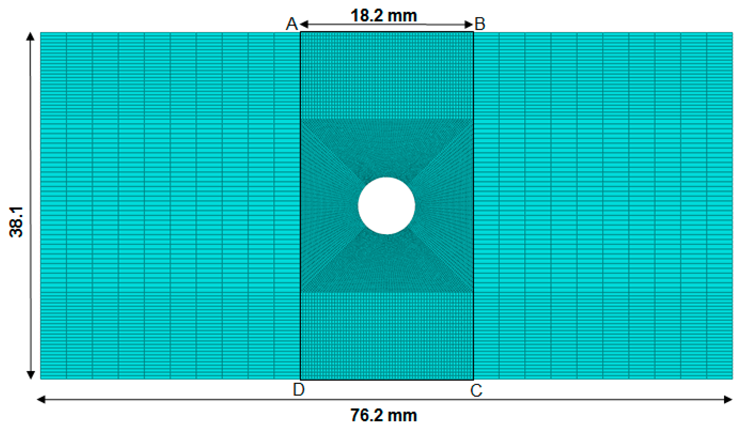
Figure 9.
Stress-strain response of the quasi-isotopic OHT specimen in pristine state and post-fatigue tested state after 106 fatigue load cycles (R = 0.1) at different specified maximum stress levels.
Figure 9.
Stress-strain response of the quasi-isotopic OHT specimen in pristine state and post-fatigue tested state after 106 fatigue load cycles (R = 0.1) at different specified maximum stress levels.
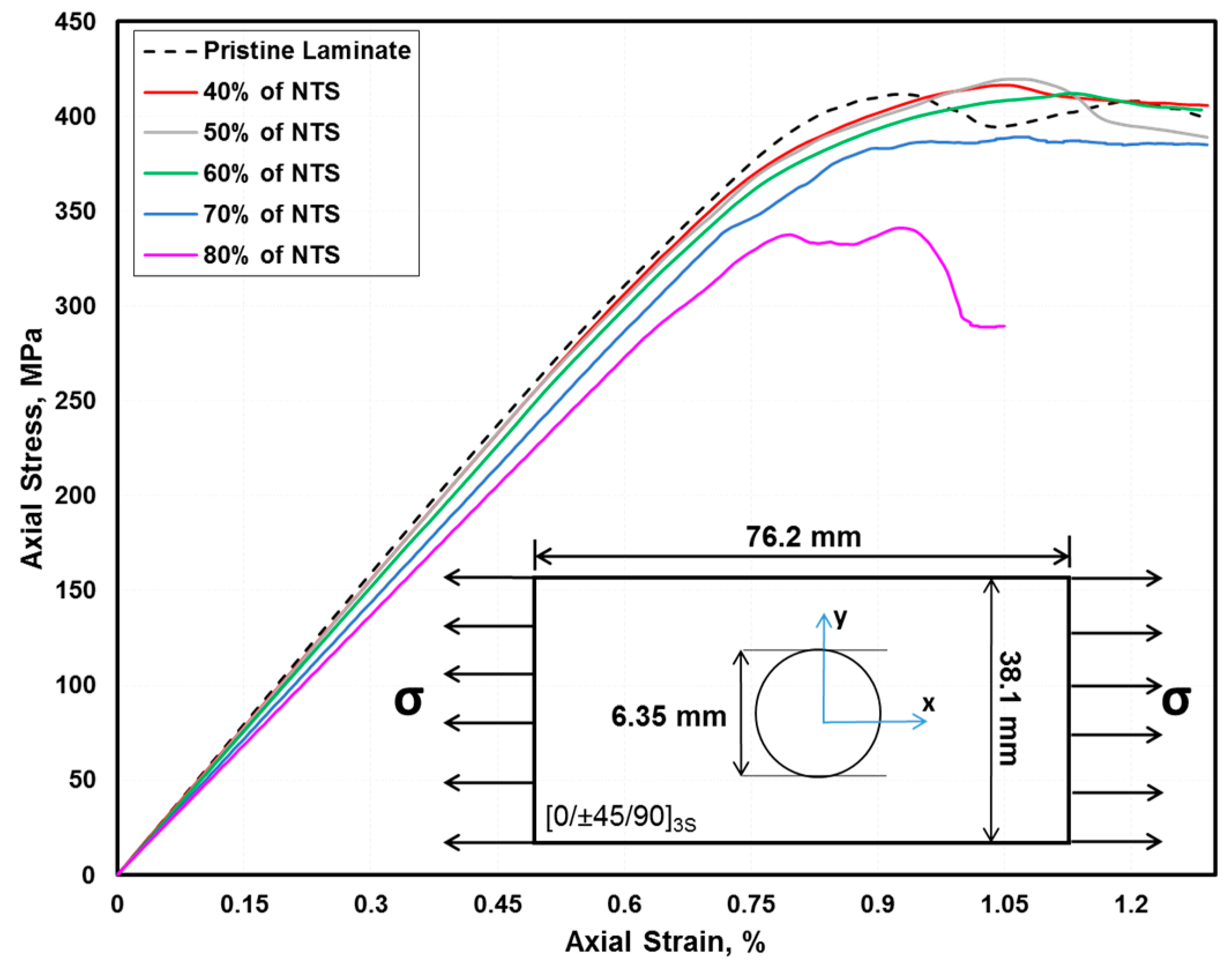
Figure 10.
Fiber tension failure index after 106 cycles in the quasi-isotropic Open Hole Tension (OHT) specimen.
Figure 10.
Fiber tension failure index after 106 cycles in the quasi-isotropic Open Hole Tension (OHT) specimen.

Figure 11.
Fiber compression failure index after 106 cycles in the quasi-isotropic OHT specimen.

Figure 12.
Matrix tension failure index after 106 cycles in the quasi-isotropic OHT specimen.

Figure 13.
Matrix compression failure index after 106 cycles in the quasi-isotropic OHT specimen.

Figure 14.
Reduction in stiffness E2 in each ply of the OHT specimen after 106 cycles.
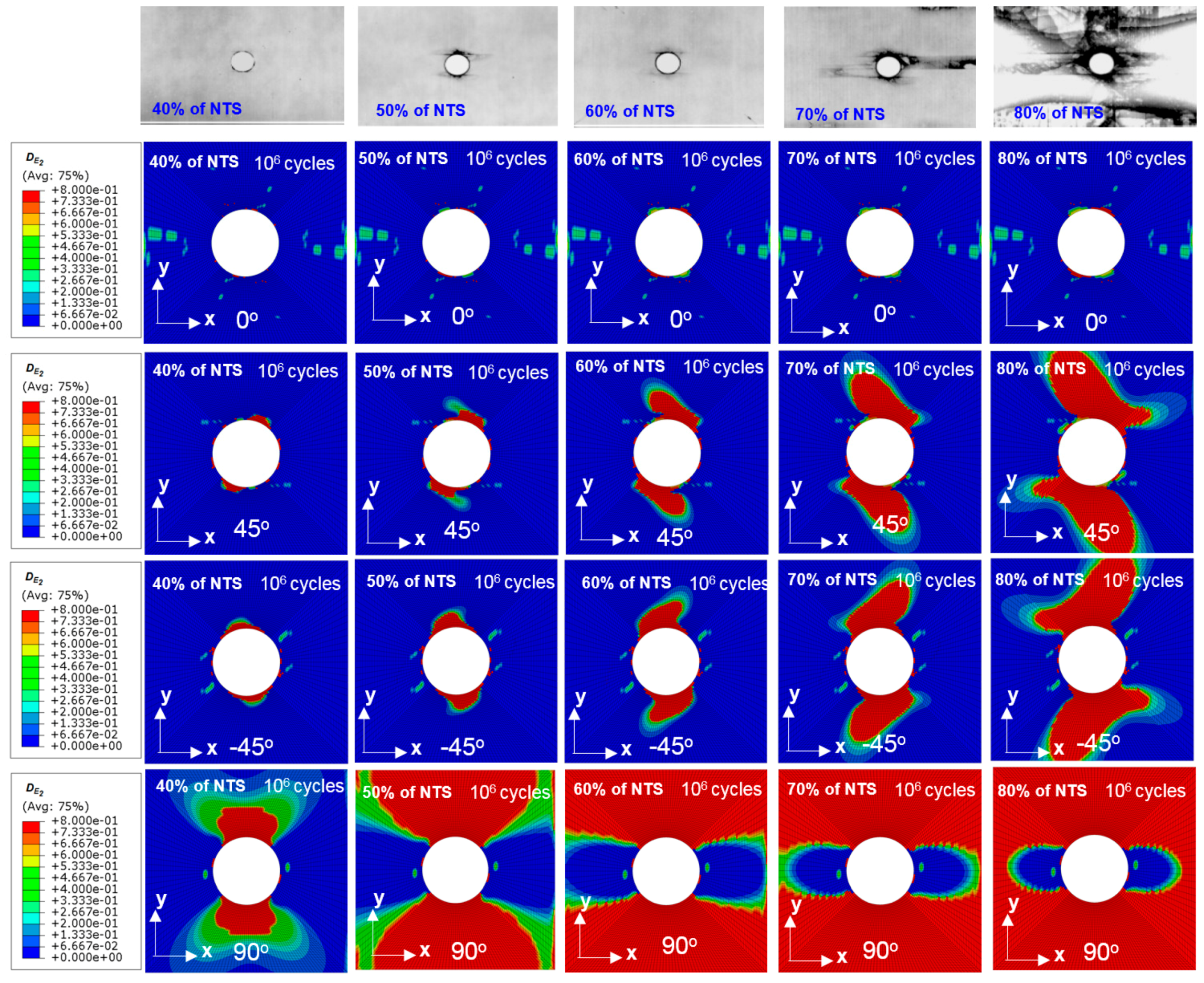
Figure 15.
Reduction in stiffness G12 in each ply of the OHT specimen after 106 cycles.
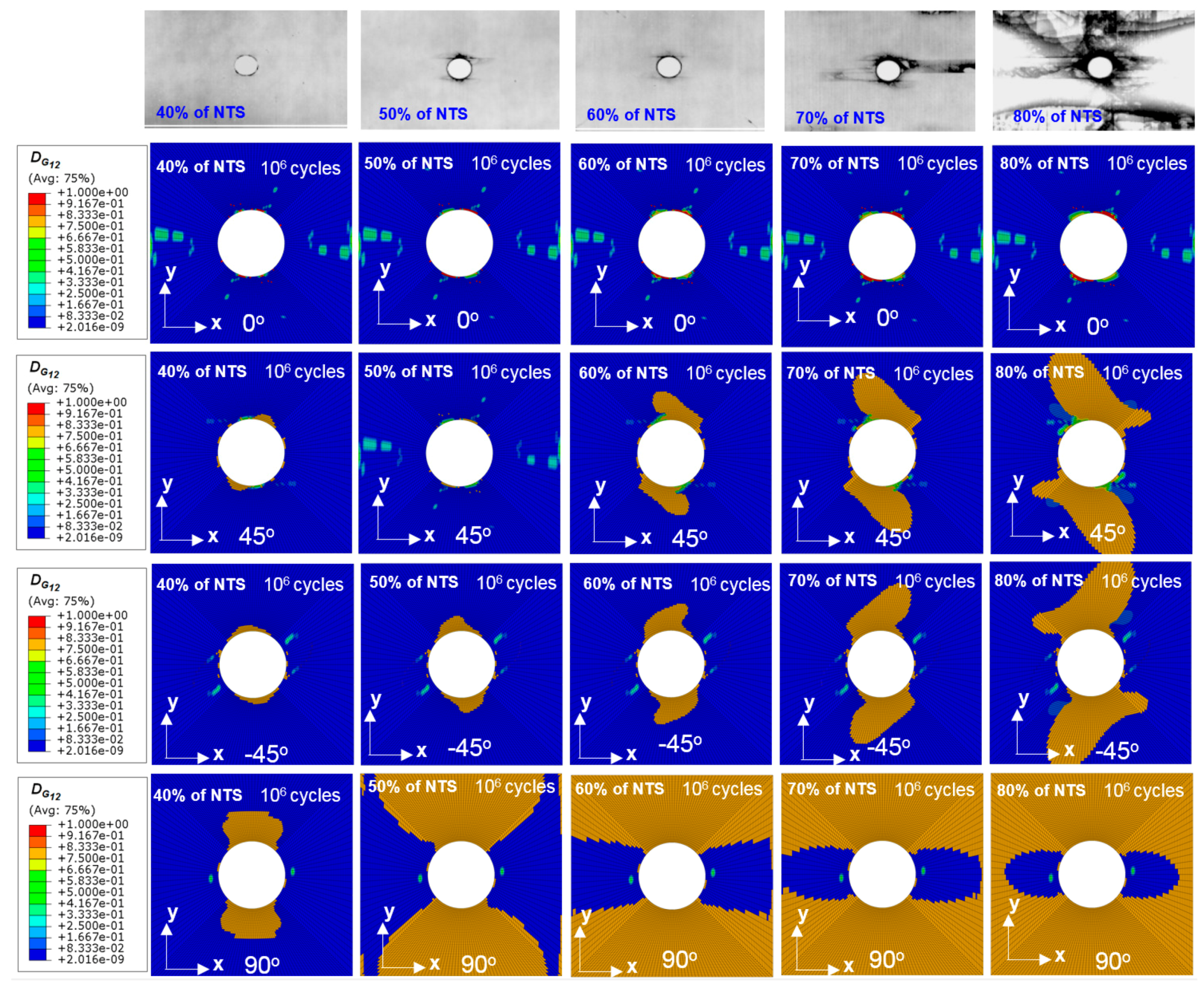
Figure 16.
Reduction in strength YT in each ply of the OHT specimen after 106 cycles.

Figure 17.
Reduction in strength S12 in each ply of the OHT specimen after 106 cycles.

Figure 18.
Reduction in strength S23 in each ply of the OHT specimen after 106 cycles.
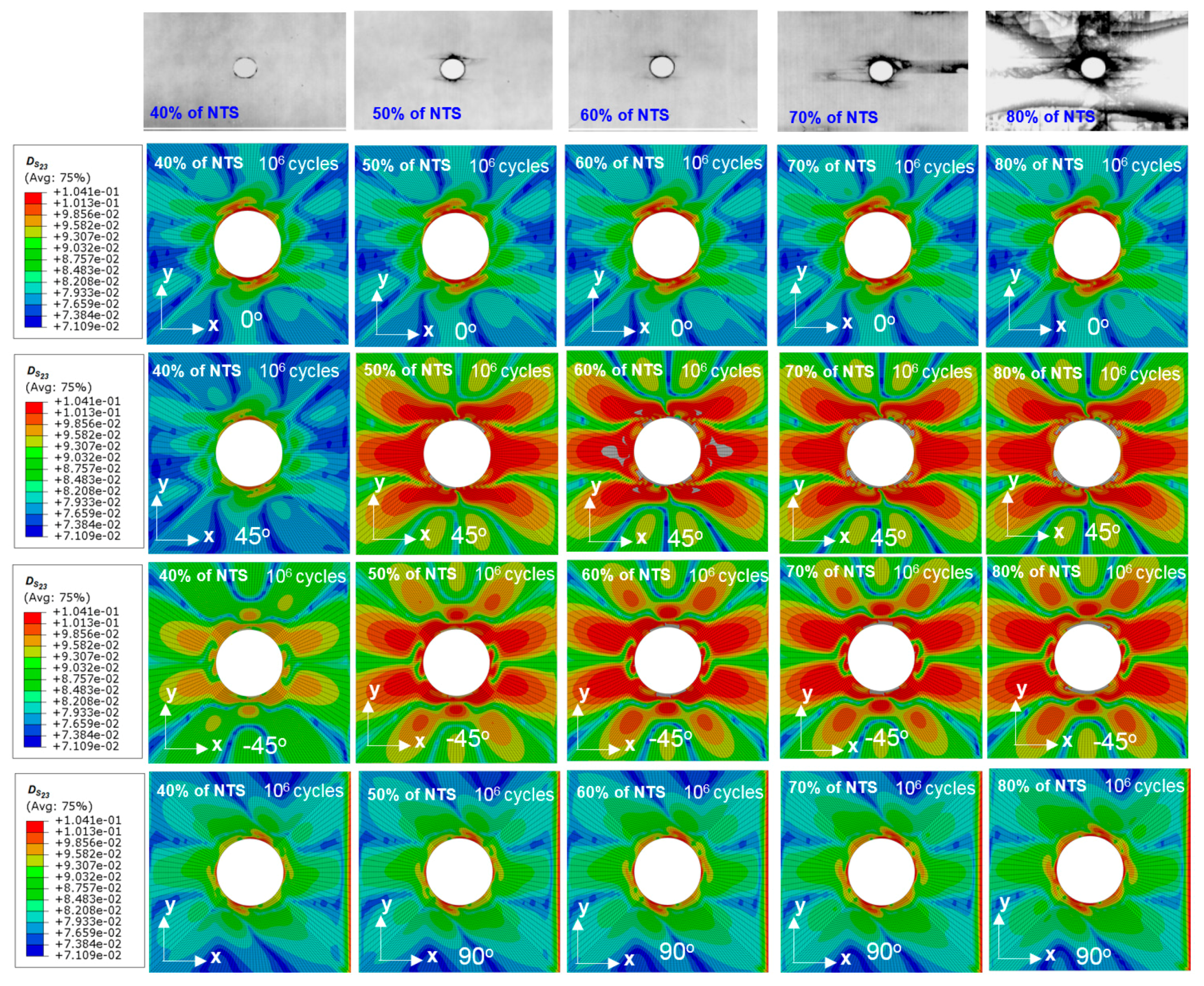
Figure 19.
Reduction in strength YT in 90° plies of the OHT specimen for increasing fatigue cycles.

Figure 20.
Reduction in stiffness G12 in 90° plies of the OHT specimen for increasing fatigue cycles.
Figure 20.
Reduction in stiffness G12 in 90° plies of the OHT specimen for increasing fatigue cycles.


Table 1.
A comparison to the values of the unified load parameters.
| Stress Level | u (Shokrieh’s Model) | Nf (Shokrieh’s Model) | u (Modified) | Nf (Modified) |
|---|---|---|---|---|
| 90% of YT | −1.2247 | 6.8624 × 10⁻²⁴ | 1.20938 | 155.394 |
| 80% of YT | −1.2344 | 5.6997 × 10⁻²⁴ | 1.33436 | 3114.24 |
| 70% of YT | −1.2671 | 2.4325 × 10⁻²⁴ | 1.47316 | 86931.2 |
| 60% of YT | −1.3282 | 5.7220 × 10⁻²⁵ | 1.62986 | 3.7281 × 10⁶ |
| 50% of YT | −1.4151 | 7.1256 × 10⁻²⁶ | 1.81064 | 2.8482 × 10⁸ |
Table 2.
Fatigue material constants in Shokrieh model for AS4 3501-6.
| Test | λ | γ | εf | α | β | A | B |
|---|---|---|---|---|---|---|---|
| Longitudinal tension | 14.57 | 0.3024 | 0.0136 | 0.473 | 10.03 | 1.3689 | 0.1097 |
| Longitudinal compression | 14.57 | 0.3024 | 0.0136 | 0.025 | 49.06 | 1.3689 | 0.1097 |
| Transverse tension | 14.57 | 0.1155 | 0.0068 | 0.1255 | 9.628 | 0.999 | 0.096 |
| Transverse compression | 14.57 | 0.1155 | 0.0068 | 0.0011 | 67.36 | 0.999 | 0.096 |
| In-plane shear | 0.70 | 11 | 0.101 | 9.11 | 0.16 | 0.0999 | 0.186 |
| Out-of-plane shear | 0.70 | 11 | 0.101 | 12 | 0.20 | 0.0999 | 0.111 |
Table 3.
Material properties to be degraded based on the mode of failure.
| Failure Mode | E1 | E2 | E3 | G12 | G13 | G23 |
|---|---|---|---|---|---|---|
| Fiber tension | 0.07 | - | - | |||
| Fiber compression | 0.14 | - | - | |||
| Matrix tension | - | 0.2 | 0.2 | 0.2 | 0.2 | 0.2 |
| Matrix compression | - | 0.4 | 0.4 | 0.4 | 0.4 | 0.4 |
Table 4.
Static material properties.
| Material Properties | Strength Parameters | ||
|---|---|---|---|
| E1 | 147 GPa | XT | 2000 MPa |
| E2 | 9 GPa | XC | 1200 MPa |
| E3 | 9 GPa | YT | 53 MPa |
| ν12 | 0.278 | YC | 204 MPa |
| ν13 | 0.278 | ZT | 53 MPa |
| ν23 | 0.40 | ZC | 204 MPa |
| G12 | 5 GPa | SXY | 137 MPa |
| G13 | 5 GPa | SXZ | 137 MPa |
| G23 | 5 GPa | SYZ | 42 MPa |
Table 5.
Comparison of the residual strength of the Open Hole Tension (OHT) specimen with test data [34].
Table 5.
Comparison of the residual strength of the Open Hole Tension (OHT) specimen with test data [34].
| Fatigue Loading Maximum Stress Level for R = 0.1, & 106 cycles | RTS Predicted (MPa) | RTS from Test (3 Replicates) (MPa) |
|---|---|---|
| 40% of NTS | 416 | 441, 461, 490 |
| 50% of NTS | 413 | 448, 468, 500 |
| 60% of NTS | 418 | 425, 445, 480 |
| 70% of NTS | 410 | 440, 467, 487 |
| 80% of NTS | 360 | 393, 412, 413 |
© 2018 by the authors. Licensee MDPI, Basel, Switzerland. This article is an open access article distributed under the terms and conditions of the Creative Commons Attribution (CC BY) license (http://creativecommons.org/licenses/by/4.0/).
Share and Cite
MDPI and ACS Style
Khan, A.I.; Venkataraman, S.; Miller, I. Predicting Fatigue Damage of Composites Using Strength Degradation and Cumulative Damage Model. J. Compos. Sci. 2018, 2, 9. https://doi.org/10.3390/jcs2010009
AMA Style
Khan AI, Venkataraman S, Miller I. Predicting Fatigue Damage of Composites Using Strength Degradation and Cumulative Damage Model. Journal of Composites Science. 2018; 2(1):9. https://doi.org/10.3390/jcs2010009
Chicago/Turabian StyleKhan, Arafat I., Satchi Venkataraman, and Ian Miller. 2018. "Predicting Fatigue Damage of Composites Using Strength Degradation and Cumulative Damage Model" Journal of Composites Science 2, no. 1: 9. https://doi.org/10.3390/jcs2010009