Multi-Objective Patch Optimization with Integrated Kinematic Draping Simulation for Continuous–Discontinuous Fiber-Reinforced Composite Structures

Abstract
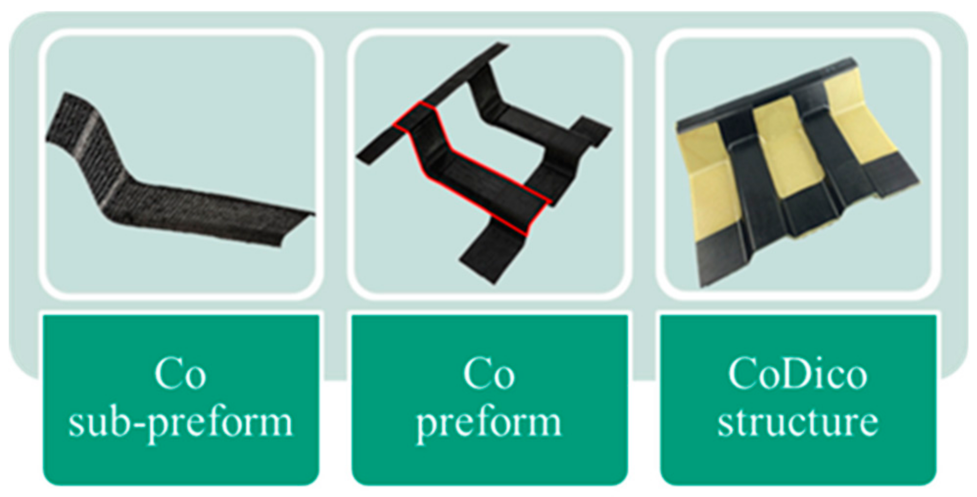
:1. Introduction
2. Draping Simulation
2.1. Suitability of Existing Draping Simulation Methods for Optimization
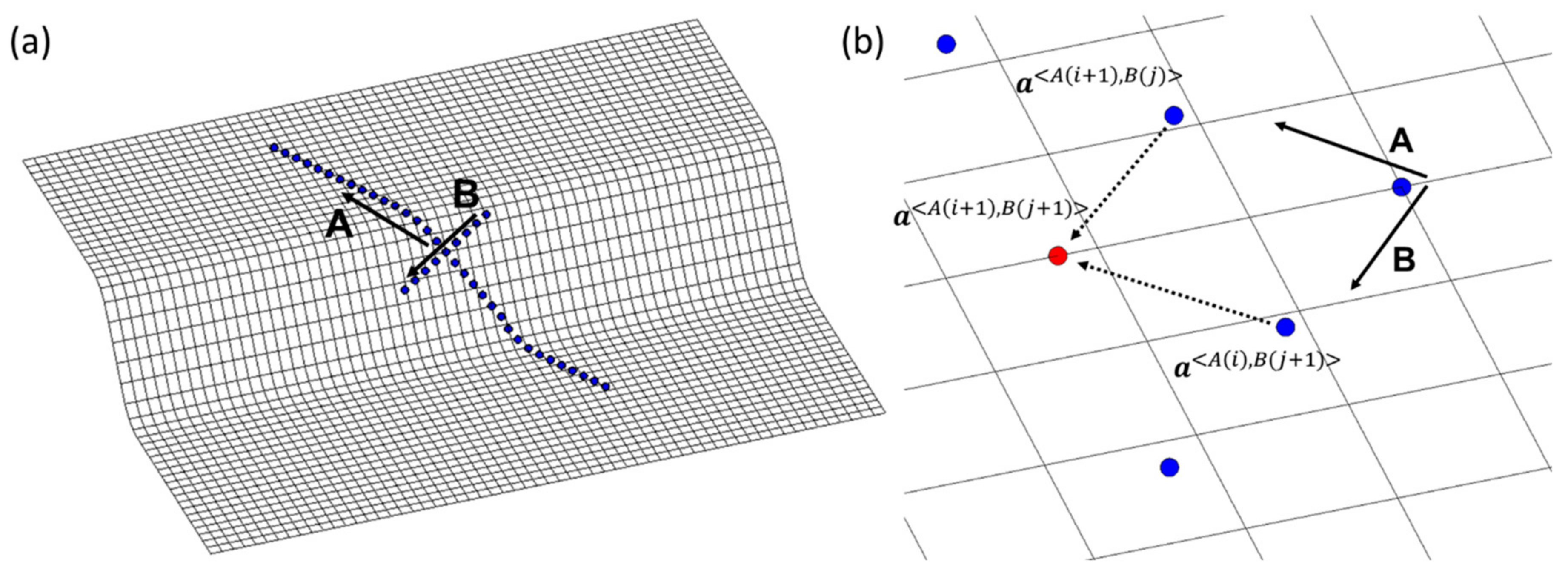
2.2. Kinematic Draping Algorithm to Be Embedded in the Optimization Workflow
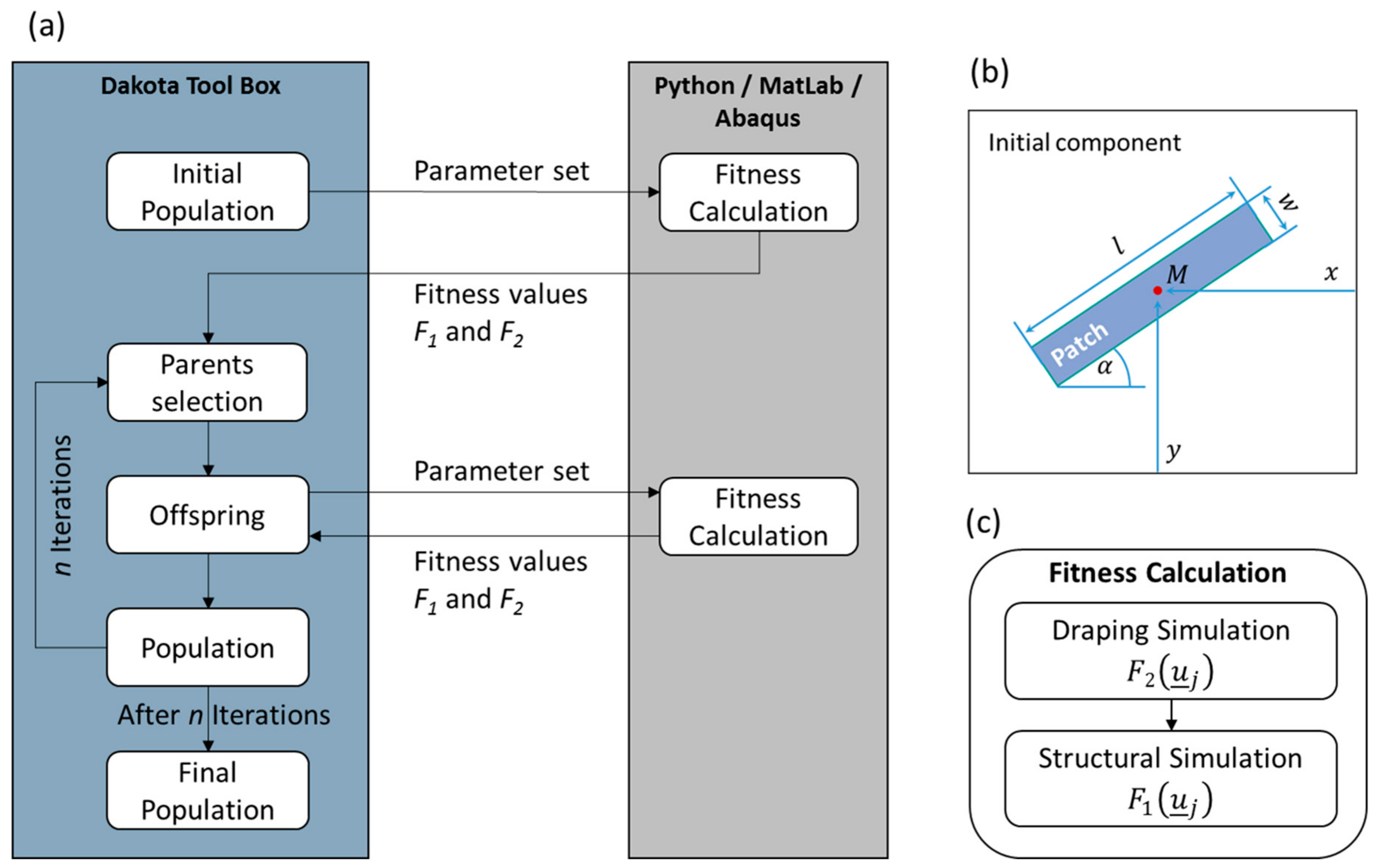
3. Multi-Objective Patch Optimization Workflow
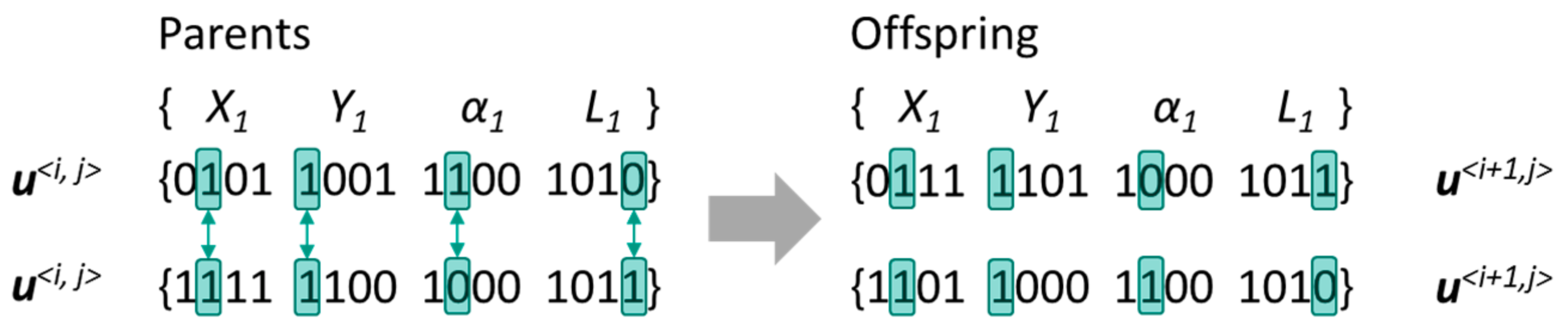
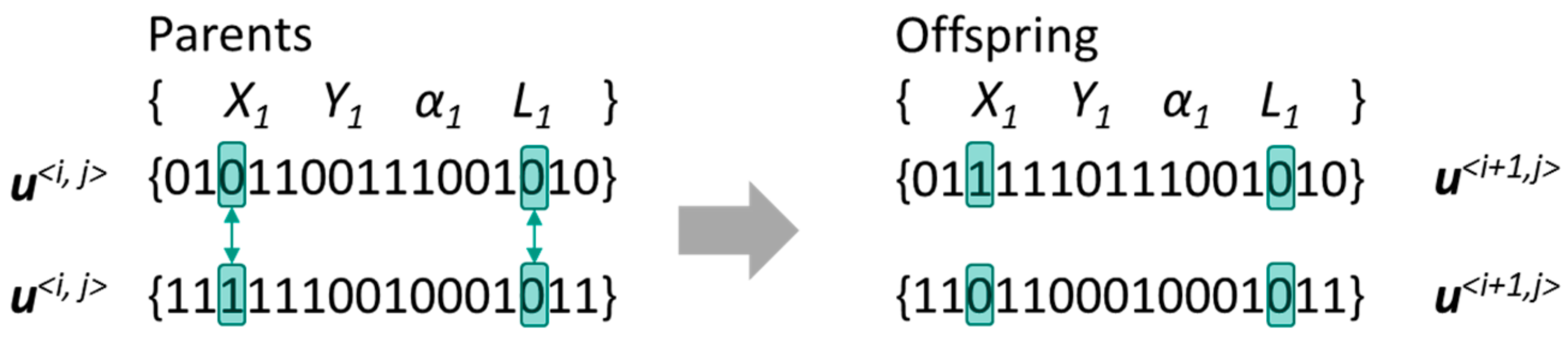
3.1. Genetic Algorithms for Multi-Objective Optimization
3.2. Patch Optimization Workflow with Embedded Kinematic Draping Simulation
- The patch fits completely on the DiCoFRP component: Here the patch usage is equal to the design parameter, representing the patch length.
- The patch does not fit completely on the DiCoFRP component: Here the patch is cut at the boarder of the component and the resulting length is returned as F2.
3.3. Convergence Criteria
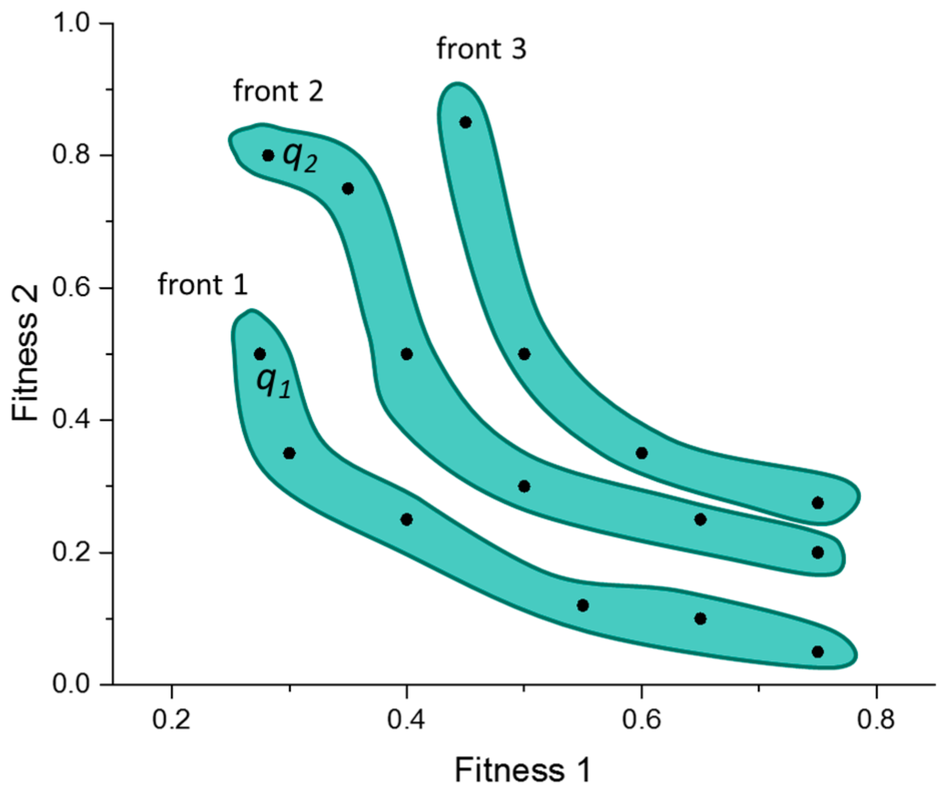
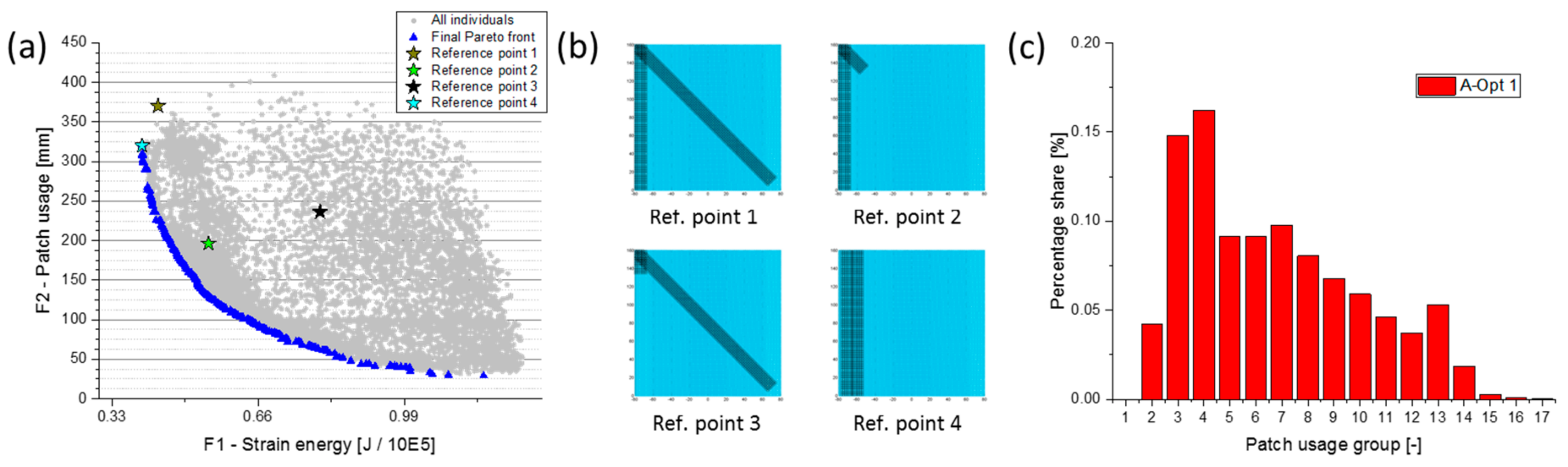
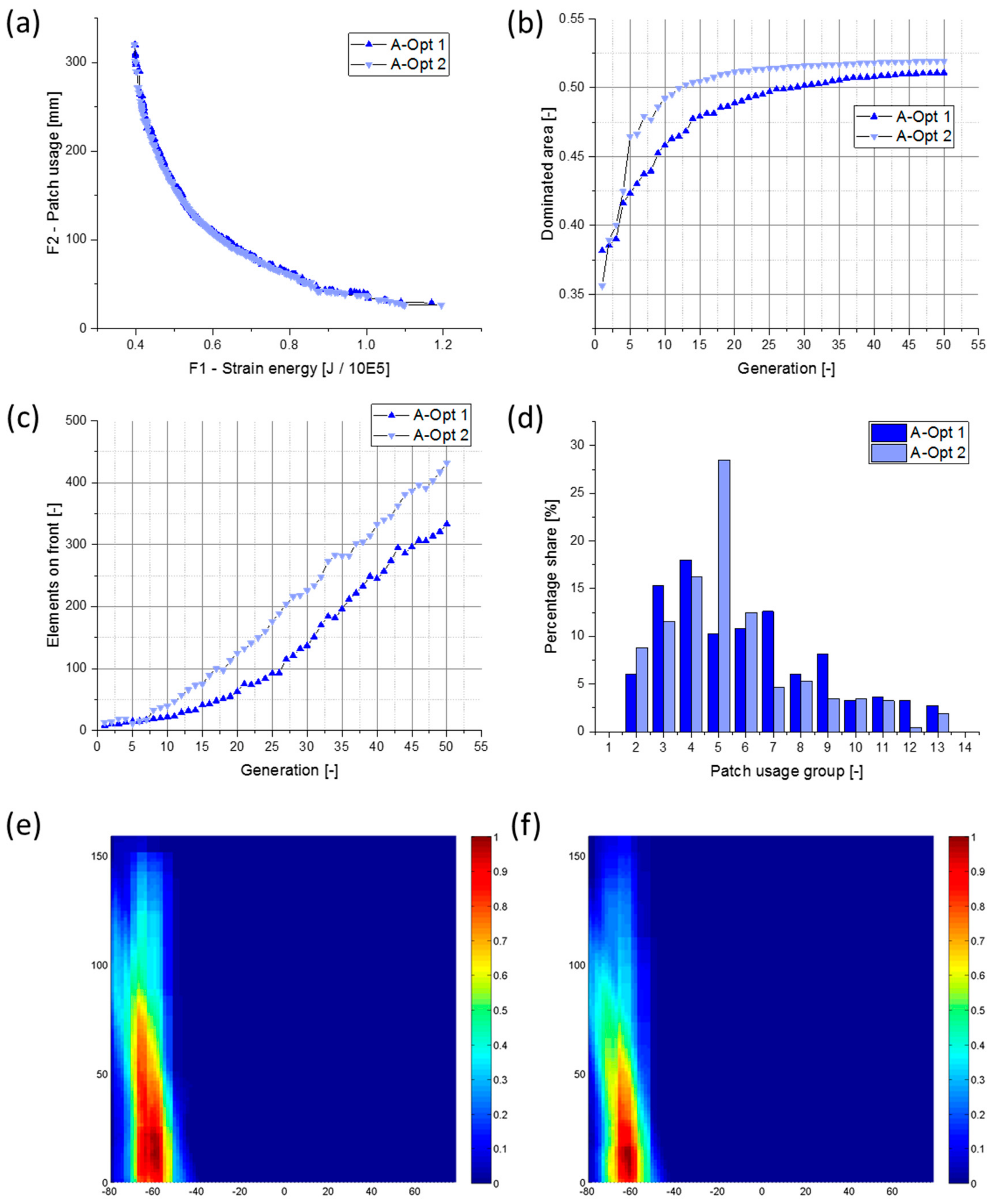
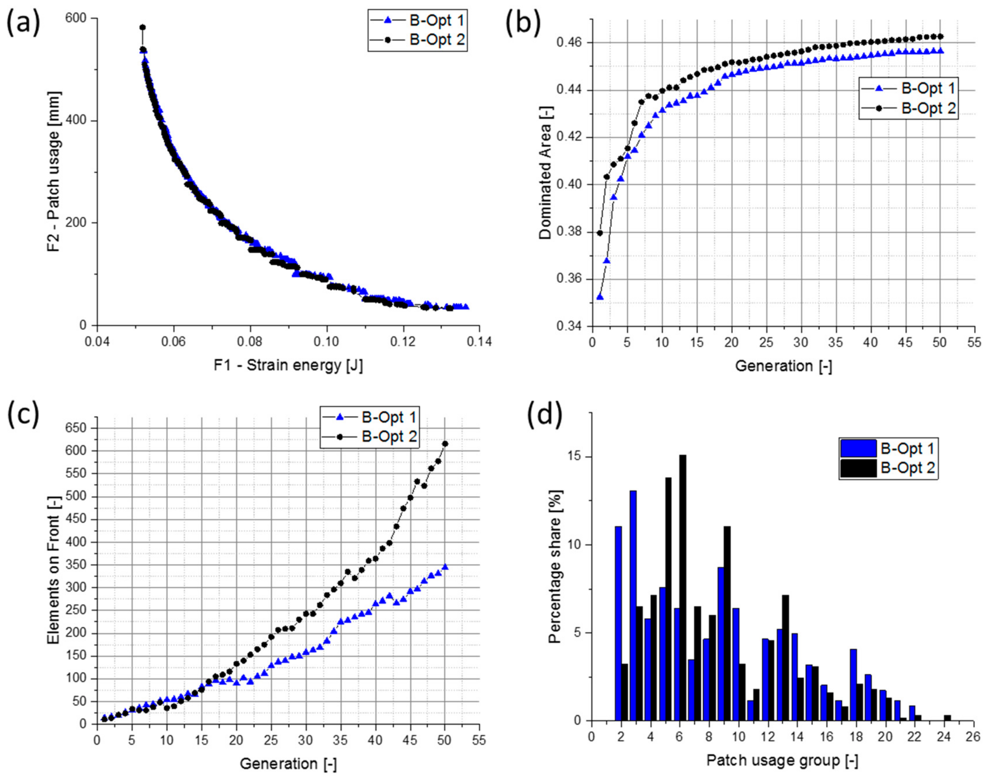
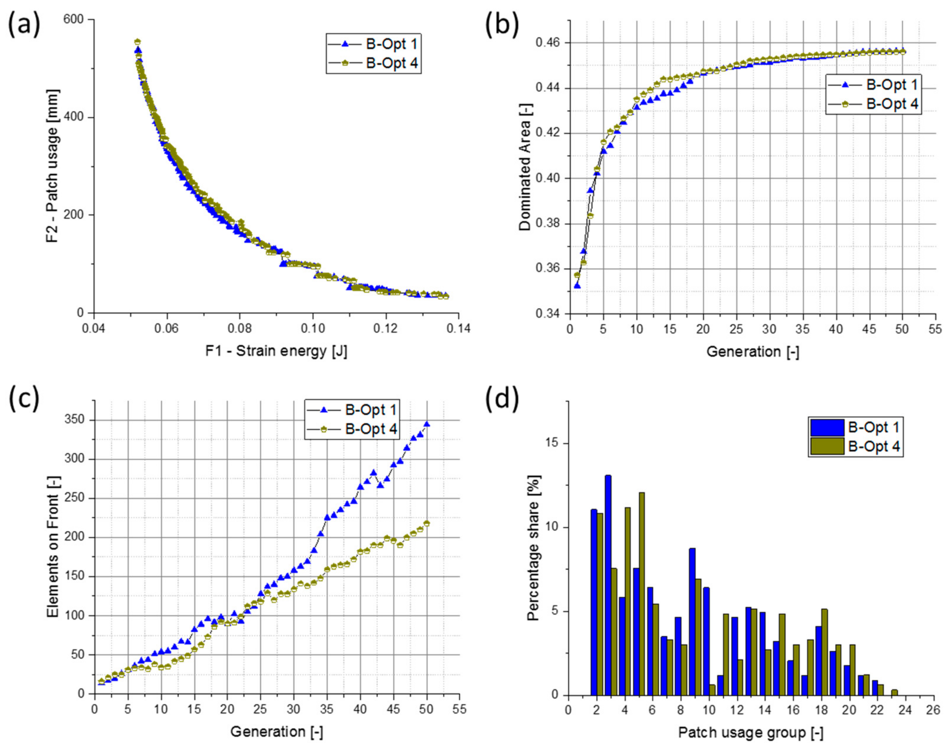
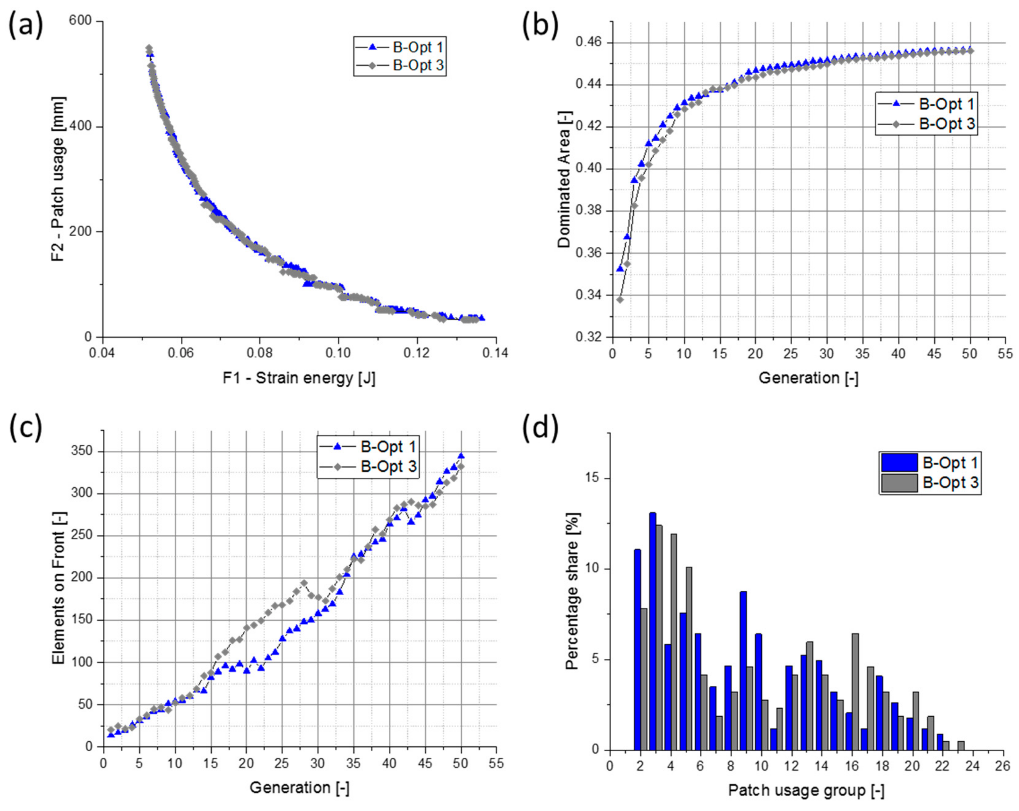
- Dominated area for the evaluation of the convergence rate. The dominated area is defined as the area enclosed by the current front and the extreme points and and therefore represents the progress of the optimization, cf. Figure 8. The extreme points are defined by
- Number of solutions along the Pareto front.
- Patch length distribution. The patch length is modeled as a discrete design variable. Therefore, the percentage share of the patch length partitions along the Pareto front is used to describe the distribution along the front.
4. Application Examples
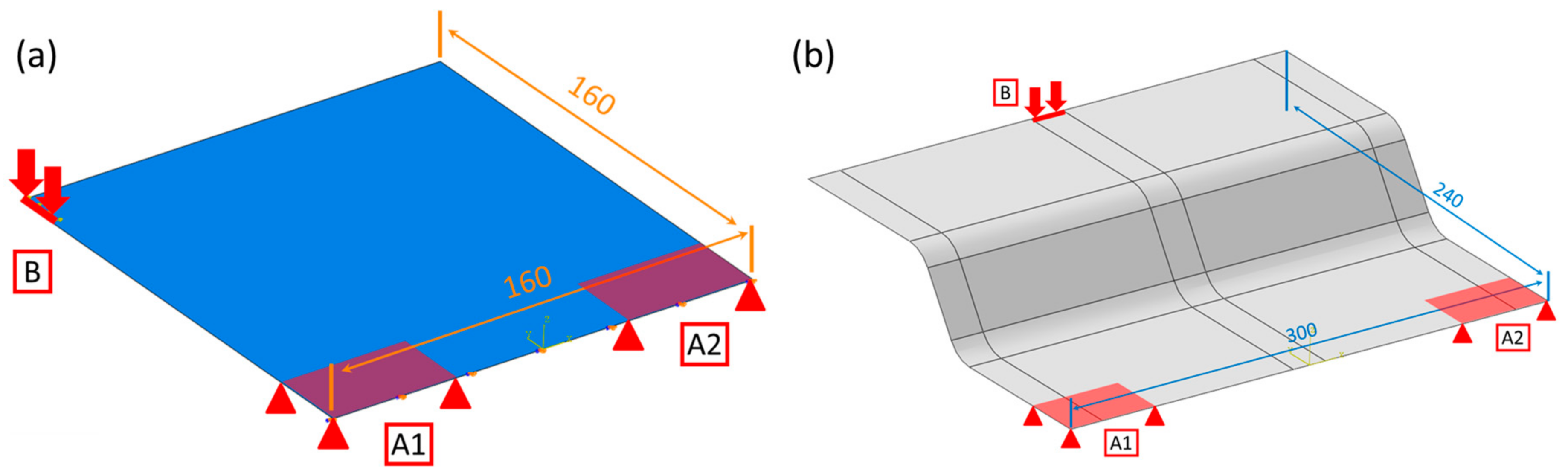
4.1. Problem Description and Optimization Parameter
4.2. Results and Discussion for the Flat Plate Example
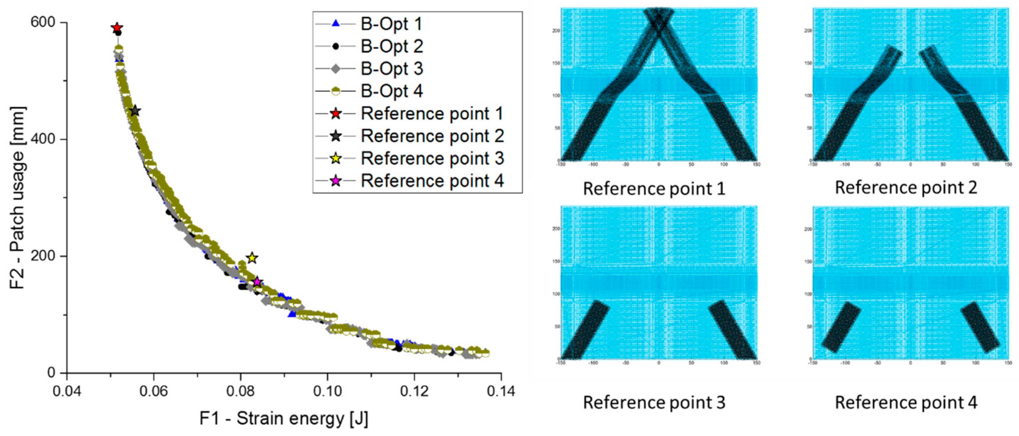
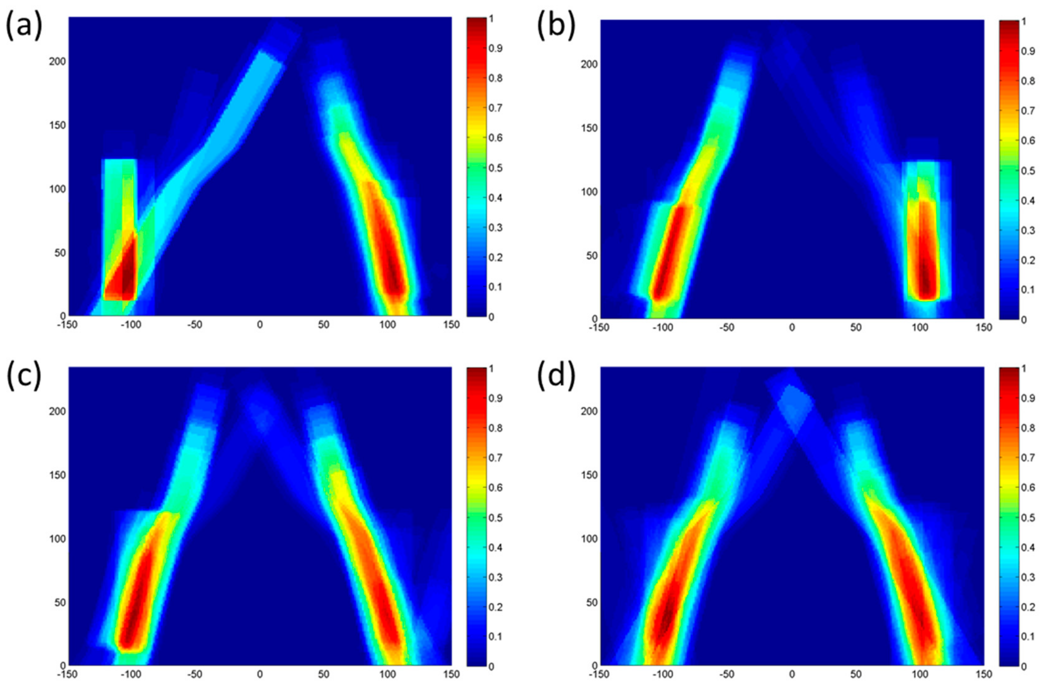
4.3. Results and Discussion for the Curved Structure Example
5. Conclusions
Acknowledgments
Author Contributions
Conflicts of Interest
References
- Bücheler, D.; Trauth, A.; Damm, A.; Böhlke, T.; Henning, F.; Kärger, L.; Seelig, T.; Weidenmann, K.A. Processing of continuous-discontinuous-fiber-reinforced thermosets. In Proceedings of the SAMPE Europe Conference, Stuttgart, Germany, 14–16 November 2017. [Google Scholar]
- Zhou, M.; Kemp, M.; Yancey, R.; Mestres, E.; Mouillet, J. Applications of Advanced Composite Simulation and Design Optimization. Altair Eng. 2011. [Google Scholar]
- Allaire, G.; Delgado, G. Stacking sequence and shape optimization of laminated composite plates via a level-set method. J. Mech. Phys. Solids 2016, 97, 168–196. [Google Scholar] [CrossRef]
- Saitou, K.; Izui, K.; Nishiwaki, S.; Papalambros, P. A Survey of Structural Optimization in Mechanical Product Development. J. Comput. Inf. Sci. Eng. 2005, 5, 214–226. [Google Scholar] [CrossRef]
- Huang, X.; Xie, Y.M. Topology optimization of nonlinear structures under displacement loading. Eng. Struct. 2008, 30, 2057–2068. [Google Scholar] [CrossRef]
- Qian, C.C.; Harper, L.T.; Turner, T.A.; Warrior, N.A. Structural optimisation of random discontinuous fibre composites: Part 1—Methodology. Compos. Part A Appl. Sci. Manuf. 2015, 68, 406–416. [Google Scholar] [CrossRef]
- Qian, C.C.; Harper, L.T.; Turner, T.A.; Warrior, N.A. Structural optimisation of random discontinuous fibre composites: Part 2—Case study. Compos. Part A Appl. Sci. Manuf. 2015, 68, 417–424. [Google Scholar] [CrossRef]
- Harzheim, L. Strukturoptimierung: Grundlagen und Anwendungen, 2nd ed.; Europa-Lehrmittel: Haan-Gruiten, Germany, 2014. [Google Scholar]
- Marler, R.T.; Arora, J.S. The weighted sum method for multi-objective optimization: New insights. Struct. Multidiscip. Optim. 2010, 41, 853–862. [Google Scholar] [CrossRef]
- Zuo, K.; Chen, L.; Zhang, Y.; Yang, J. Manufacturing- and machining-based topology optimization. Int. J. Adv. Manuf. Tech. 2006, 27, 531–536. [Google Scholar] [CrossRef]
- Sørensen, S.N.; Lund, E. Topology and thickness optimization of laminated composites including manufacturing constraints. Struct. Multidiscip. Optim. 2013, 48, 249–265. [Google Scholar] [CrossRef]
- Zein, S.; Madhavan, V.; Dumas, D.; Ravier, L.; Yague, I. From stacking sequences to ply layouts: An algorithm to design manufacturable composite structures. Compos. Struct. 2016, 141, 32–38. [Google Scholar] [CrossRef]
- Zhou, M.; Fleury, R.; Shyy, Y.; Thomas, H.; Brennan, J. Progress in Topology Optimization with Manufacturing Constraints. In Proceedings of the 9th AIAA/ISSMO Symposium on Multidisciplinary Analysis and Optimization, Atlanta, GA, USA, 4–6 September 2002. [Google Scholar]
- Hohberg, M.; Kärger, L.; Henning, F.; Hrymak, A. Process Simulation of Sheet Molding Compound (SMC) as key for the integrated Simulation Chain. In Proceedings of the Simulation of Composites—Ready for Industry 4.0? Hamburg, Germany, 24–27 October 2016; pp. 61–67. [Google Scholar]
- Kärger, L.; Bernath, A.; Fritz, F.; Galkin, S.; Magagnato, D.; Oeckerath, A.; Schön, A.; Henning, F. Development and validation of a CAE chain for unidirectional fibre reinforced composite components. Compos. Struct. 2015, 132, 350–358. [Google Scholar] [CrossRef]
- Kaufmann, M.; Zenkert, D.; Åkermo, M. Cost/weight optimization of composite prepreg structures for best draping strategy. Compos. Part A Appl. Sci. Manuf. 2010, 41, 464–472. [Google Scholar] [CrossRef]
- Kärger, L.; Galkin, S.; Dörr, D.; Schirmaier, F.; Oeckerath, A.; Wolf, K. Continuous CAE chain for composite design, established on an HPC system and accessible via web-based user-interfaces. In Proceedings of the NAFEMS World Congress, Stockholm, Sweden, 11–14 June 2017. [Google Scholar]
- Kärger, L.; Galkin, S.; Zimmerling, C.; Dörr, D.; Linden, J.; Oeckerath, A.; Wolf, K. Forming optimisation embedded in a CAE chain to assess and enhance the structural performance of composite components. Compos. Struct. 2018. [Google Scholar] [CrossRef]
- Bulla, M.; Beauchense, E.; Ehrhart, F.; Trickov, V. A holistic simulation driven composite design process. Proc. NAFEMS Semin. Simul. 2014, in press. [Google Scholar]
- Zehnder, N.; Ermanni, P. Optimizing the shape and placement of patches of reinforcement fibers. Compos. Struct. 2007, 77, 1–9. [Google Scholar] [CrossRef]
- Zehnder, N.; Ermanni, P. A methodology for the global optimization of laminated composite structures. Compos. Struct. 2005, 72, 311–320. [Google Scholar] [CrossRef]
- Mathias, J.; Balandraud, X.; Grediac, M. Applying a genetic algorithm to the optimization of composite patches. Comput. Struct. 2006, 84, 823–834. [Google Scholar] [CrossRef]
- Mejlej, V.G.; Falkenberg, P.; Türck, E.; Vietor, T. Optimization of Variable Stiffness Composites in Automated Fiber Placement Process using Evolutionary Algorithms. Procedia CIRP 2017, 66, 79–84. [Google Scholar] [CrossRef]
- Jansson, N.; Wakeman, W.D.; Månson, J.E. Optimization of hybrid thermoplastic composite structures using surrogate models and genetic algorithms. Compos. Struct. 2007, 80, 21–31. [Google Scholar] [CrossRef]
- Skordos, A.A.; Sutcliffe, M.P.F.; Klintworth, J.W.; Adolfsson, P. Multi-Objective Optimisation of Woven Composite Draping using Genetic Algorithms. In Proceedings of the 27th International Conference SAMPE Europe, Paris, France, 27–29 March 2006. [Google Scholar]
- Chen, S.; Harper, L.T.; Endruweit, A.; Warrior, N.A. Formability optimisation of fabric preforms by controlling material draw-in through in-plane constraints. Compos. Part A Appl. Sci. Manuf. 2015, 76, 10–19. [Google Scholar] [CrossRef]
- Lim, T.; Ramakrishna, S. Modelling of composite sheet forming: A review. Compos. Part A Appl. Sci. Manuf. 2002, 33, 515–537. [Google Scholar] [CrossRef]
- Spencer, A.J.M. Theory of fabric-reinforced viscous fluids. Compos. Part A Appl. Sci. Manuf. 2000, 31, 1311–1321. [Google Scholar] [CrossRef]
- Boisse, P.; Aimène, Y.; Dogui, A.; Dridi, S.; Gatouillat, S.; Hamila, N.; Khan, M.A.; Mabrouki, T.; Morestin, F.; Vidal-Sallé, E. Hypoelastic, hyperelastic, discrete and semi-discrete approaches for textile composite reinforcement forming. Int. J. Mater. Form. 2010, 3, 1229–1240. [Google Scholar] [CrossRef]
- Dörr, D.; Schirmaier, F.J.; Henning, F.; Kärger, L. A viscoelastic approach for modeling bending behavior in finite element forming simulation of continuously fiber reinforced composites. Compos. Part A Appl. Sci. Manuf. 2017, 94, 113–123. [Google Scholar] [CrossRef]
- Schirmaier, F.J.; Dörr, D.; Henning, F.; Kärger, L. A macroscopic approach to simulate the forming behaviour of stitched unidirectional non-crimp fabrics (UD-NCF). Compos. Part A Appl. Sci. Manuf. 2017, 102, 322–335. [Google Scholar] [CrossRef]
- Sharma, S.B.; Sutcliffe, M.P.F. Draping of woven fabrics: Progressive drape model. Plast. Rubber Compos. 2013, 32, 57–64. [Google Scholar] [CrossRef]
- Yang, B.; Jin, T.; Bi, F.; Li, J. A Geometry Information Based Fishnet Algorithm for Woven Fabric Draping in Liquid Composite Molding. Mater. Sci. 2014, 20, 513–521. [Google Scholar] [CrossRef]
- Smiley, A.J.; Pipes, R.B. Analysis of the Diaphragm Forming of Continuous Fiber Reinforced Thermoplastics. J. Thermoplast. Compos. Mater. 1988, 1, 298–321. [Google Scholar] [CrossRef]
- Long, A.C.; Rudd, C.D. A simulation of reinforcement deformation during the production of preforms for liquid moulding processes. Proc. Inst. Mech. Eng. Part B J. Eng. Manuf. 1994, 208, 269–278. [Google Scholar] [CrossRef]
- Pickett, A.K.; Creech, G.; Luca, P.D. Simplified and advanced simulation methods for prediction of fabric draping. Rev. Eur. Elem. 2012, 14, 677–691. [Google Scholar] [CrossRef]
- Van West, B.P.; Pipes, R.B.; Keefe, M. A Simulation of the Draping of Bidirectional Fabrics over Arbitrary Surfaces. J. Text. Inst. 1990, 81, 448–460. [Google Scholar] [CrossRef]
- Vanclooster, K.; Lomov, S.V.; Verpoest, I. Simulating and validating the draping of woven fiber reinforced polymers. Int. J. Mater. Form. 2008, 1, 961–964. [Google Scholar] [CrossRef]
- Bäck, T. Evolutionary Algorithms in Theory and Practice: Evolution Strategies, Evolutionary Programming, Genetic Algorithms; Oxford University Press: Oxford, UK, 1996. [Google Scholar]
- Coello, C.A. A Short Tutorial on Evolutionary Multiobjective Optimization. In International Conference on Evolutionary Multi-Criterion Optimization; Springer: Berlin/Heidelberg, Germany, 2001; pp. 21–40. [Google Scholar]
- Giger, M. Representation Concepts in Evolutionary Algorithm-Based Structural Optimization. Ph.D. Thesis, Zürich, Switzerland, 2007. [Google Scholar]
- Adams, B.M.; Bauman, L.E.; Bohnhoff, W.J.; Dalbey, K.R.; Ebeida, M.S.; Eddy, J.P.; Eldred, M.S.; Hough, P.D.; Hu, K.T.; Jakeman, J.D.; et al. Dakota, A Multilevel Parallel Object-Oriented Framework for Design Optimization, Parameter Estimation, Uncertainty Quantification, and Sensitivity Analysis: Version 6.0 User’s Manual. July 2014; Updated November 2015 (Version 6.3). Sandia Technical Report SAND2014-4633. Available online: https://dakota.sandia.gov/content/citing-dakota (accessed on 13 March 2017).


| Name | Structure | Crossover | Mutation | Replacement | Niching |
|---|---|---|---|---|---|
| A-Opt 1 | Plate | Parameterized binary | High | Elitist | No |
| A-Opt 2 | Plate | Multi-point binary | High | Elitist | No |
| B-Opt 1 | Curved shell | Multi-point binary | Low | Elitist | No |
| B-Opt 2 | Curved shell | Multi-point binary | High | Elitist | No |
| B-Opt 3 | Curved shell | Multi-point binary | Low | Below limit | No |
| B-Opt 4 | Curved shell | Multi-point binary | Low | Elitist | Yes |
© 2018 by the authors. Licensee MDPI, Basel, Switzerland. This article is an open access article distributed under the terms and conditions of the Creative Commons Attribution (CC BY) license (http://creativecommons.org/licenses/by/4.0/).
Share and Cite
Fengler, B.; Kärger, L.; Henning, F.; Hrymak, A. Multi-Objective Patch Optimization with Integrated Kinematic Draping Simulation for Continuous–Discontinuous Fiber-Reinforced Composite Structures. J. Compos. Sci. 2018, 2, 22. https://doi.org/10.3390/jcs2020022
Fengler B, Kärger L, Henning F, Hrymak A. Multi-Objective Patch Optimization with Integrated Kinematic Draping Simulation for Continuous–Discontinuous Fiber-Reinforced Composite Structures. Journal of Composites Science. 2018; 2(2):22. https://doi.org/10.3390/jcs2020022
Chicago/Turabian StyleFengler, Benedikt, Luise Kärger, Frank Henning, and Andrew Hrymak. 2018. "Multi-Objective Patch Optimization with Integrated Kinematic Draping Simulation for Continuous–Discontinuous Fiber-Reinforced Composite Structures" Journal of Composites Science 2, no. 2: 22. https://doi.org/10.3390/jcs2020022