Prediction of the Fiber Orientation State and the Resulting Structural and Thermal Properties of Fiber Reinforced Additive Manufactured Composites Fabricated Using the Big Area Additive Manufacturing Process

Abstract

Recent advances in Fused Filament Fabrication (FFF) include large material deposition rates and the addition of chopped carbon fibers to the filament feedstock. During processing, the flow field within the polymer melt orients the fiber suspension, which is important to quantify as the underlying fiber orientation influences the mechanical and thermal properties. This paper investigates the correlation between processing conditions and the resulting locally varying thermal-structural properties that dictate both the final part performance and part dimensionality. The flow domain includes both the confined and unconfined flow indicative of the extruder nozzle within the FFF deposition process. The resulting orientation is obtained through two different isotropic rotary diffusion models, the model by Folgar and Tucker and that of Wang et al., and a comparison is made to demonstrate the sensitivity of the deposited bead’s spatially varying orientation as well as the final processed part’s thermal-structural performance. The results indicate the sensitivity of the final part behavior is quite sensitive to the choice of the slowness parameter in the Wang et al. model. Results also show the need, albeit less than that of the choice of fiber interaction model, to include the extrudate swell and deposition within the flow domain.

1. Introduction

Fused Filament Fabrication (FFF) is an Additive Manufacturing (AM) technology that extrudes beads of thermoplastic materials onto a moving substrate, layer by layer, based on a digital three-dimensional model. Since its introduction nearly three decades ago, FFF (sometimes called Fused Deposition Modeling or FDM^TM) has become one of the fastest growing forms of AM. An attractive feature of FFF as compared to other AM systems is material selection (see e.g., [1]). While this advantage is responsible, in part, for the growth of FFF, the lack of structural materials and scalability to industrially relevant volumes are limiting factors that must be overcome in order to realize widespread application of AM systems. Recently, large scale FFF processes such as the Big Area Additive Manufacturing (BAAM) process developed at the Manufacturing Demonstration Facility (MDF) at Oak Ridge National Laboratories has significantly increased build volume. In addition, fiber reinforcements have recently been introduced in FFF systems to reduce distortion and improve the mechanical performance of the final part, particularly in the Z- or through-thickness direction where they are weak. This work seeks to quantify the intra-layer structural and thermal performance of the deposited bead. The inter-layer performance is another significant consideration, and there are a variety of authors who have presented methods to improve the inter-layer bonding strength such as tamping (see e.g., [2,3]), infrared preheating (see e.g., [4]), and plasma treating (see e.g., [5]).

Fiber reinforced matrix (FRM) composites are used in many industries using multiple manufacturing processes. For example, FRM composites have been used in construction for many years (see e.g., [6]). They have also been used in the aerospace and medical industries (see e.g., [7,8,9]). In addition, the use of short-fiber reinforced composites is widely prevalent throughout the injection and compression molding community and is the most closely related field to the present work. The significant difference between the presented work and previous modeling efforts of molding processes is that FFF systems have a closed cavity flow followed by an unconfined expansion with a subsequent confined boundary from the moving plate.

With the recent advances of large scale FFF, the use of fiber reinforcements in the AM process is a viable option for increasing the performance of AM parts (see e.g., [10,11]). The process of blending short, chopped fibers into a polymer melt coupled with the freeform nature of AM allows for the fabrication of complex and intricate parts with the potential for improved structural performance and with a geometric complexity previously unavailable. A key aspect to realize this vision is understanding the impact of the nozzle, both its geometry and position relative to the moving platen, on the internal fiber orientation state within the deposited bead and, by extension, the part’s final stiffness. The thermo-mechanical behavior of the bead is also quite critical as the deposition process induces large thermal gradients during fabrication and can impact the final part’s dimensionality. To quantify a-priori the distortion of the entire fabricated product, the spatially and directionally varying anisotropic stiffness and coefficient of thermal expansion tensors would be required. This work seeks to present a method to predict the anisotropic stiffness and thermal expansion tensors due to local variations in the fiber microstructure. The results from this paper can be used in a full scale simulation of the macroscopic fabricated product, and the methodology presented in this work can be used by designers in establishing new nozzle designs for the extruder to tailor the properties of the deposited bead.

Fiber microstructure predictions in a short-fiber reinforced polymer composite require an accurate understanding of the relationship between the fiber kinetics and the flow kinematics. There is an extensive body of literature to address the relationship between the local fiber orientation kinetics and the surrounding velocity field (see e.g., [12,13,14,15,16,17,18,19]). Several authors have developed methods for predicting part stiffness and thermal conductivity as a function of local fiber orientation in the hardened polymer melt (see e.g., [13,20,21,22]). Most fiber kinetics models are based on the motion of individual ellipsoids in a dilute Newtonian solvent as constructed by Jeffery [23]. It is unfeasible to track the motion of every fiber within a suspension, thus the fiber orientation distribution function (ODF) is often more desirable. The full ODF has been solved using control volumes (see e.g., Bay [24]) or the computationally efficient and numerically exact spherical harmonics (see e.g., Montgomery-Smith et al. [25]). Flow kinematics are coupled to the fiber orientation state in densely packed flows (see e.g., [26,27]) and several authors have performed numerical solutions for fully coupled flows (see e.g., [28,29]). In the present study, flow kinematics are decoupled from the fiber orientation state similar to what is often done in injection molding simulations (see e.g., [17,29,30,31]). This work focuses on the impact that the swell of the extrudate has on the final orientation state.

The kinetic equation for the ODF may be used to describe the concentrated suspension behavior of interacting fibers through the addition of a rotary diffusivity term $D_r$ as generalized by Bird et al. [32] for the related system of polymer chain alignment. The Folgar and Tucker [12] isotropic rotary diffusion (IRD) model to represent fiber interactions has been widely used for more than three decades. Recent studies demonstrate the IRD model predicts fiber alignment occurs at a rate faster than that observed experimentally and several authors have sought to address this limitation (see e.g., [15,17,18,33,34]). The strain-reduction factor model of Huynh [16] sought to reduce the alignment rate by a scaling parameter pre-multiplied on the equation of motion. The reduced strain closure model (IRD-RSC) of Wang et al. [17] expanded the Huynh [16] approach by reducing the rate of fiber alignment by operating exclusively on the eigenvalues of the orientation tensors and thus is invariant with respect to the chosen coordinate frame. Recently Phelps and Tucker [18] introduced the anisotropic rotary diffusion model (ARD) which introduces a directional dependence to fiber interactions and has been shown to be quite effective for select long-fiber systems. Unfortunately, the general behavior of the five ARD empirical coefficients as a function of the polymer melt and fiber packing is not yet well understood in the literature. Strautins and Latz [35] introduced a computationally efficient form for flexible fibers using the moments of the orientation distribution, and Ortman et al. [19] extended their work to allow fiber interactions using a strain-reduction extension of the IRD model based on the work of Sepehr et al. [34]. The current paper focuses on short, rigid fibers within a polymer melt and compares results between the classical IRD model and the recent IRD-RSC model. Particular focus is given to the sensitivity of the processed orientation state to the interaction coefficient $C_I$ within both models and the slow-down parameter $\kappa$ in the IRD-RSC model.

One objective of predicting the fiber orientation is to determine the mechanical performance of the deposited bead. Advani and Tucker [13] linked the stiffness of the solidified part to the local fiber microstructure using an orientation homogenization approach. In Jack and Smith [22] closed form expressions for the stiffness expectation and variance were derived using complex spherical harmonics. Nguyen et al. [36] performed a comparison between the $E_1$ and $E_2$ predicted by the IRD-RSC model and tensile tests. Recently Nguyen et al. [31] used the ARD model to predict the fiber orientation and the subsequent stress response for an injection molded long fiber thermoplastic. This work was extended by Agboola et al. [37] to investigate the impact the choice of fiber interaction model has on the expected macroscopic stiffness of a simple two dimensional part. Recently Stair and Jack [38] demonstrated the effectiveness of taking the measured properties of the neat polymer and fibers to predict both the locally varying stiffness and Coefficient of Thermal Expansion (CTE) tensors and then used this information to successfully predict the part warpage of laminated composites due to processing.

The current paper presents a computational approach that extends the work of Agboola et al. [37] and Stair and Jack [38] for related composite systems to predict the stiffness and CTE tensors for the deposited bead of a fiber reinforced polymer bead fabricated using the large volume FFF process. Results are presented based on predictions of the spatially varying fiber orientation obtained from process simulations that include the nozzle, die-swell and subsequent deposition and the constitutive properties of the neat polymer and individual fibers. A method is presented to predict the spatially varying, bulk stiffness tensors and CTE tensors for the beads for results from the IRD and the IRD-RSC fiber interaction models to determine the sensitivity of the final part performance to variations in fiber interaction parameters.

2. Fiber Orientation Modeling

The foundational work of Jeffery [23] describes the orientation change of a rigid and mass-less ellipsoidal particle in a fluid. The particle direction is defined by $\mathbf{p}$, a unit vector along the fiber longitudinal axis. While Jeffery’s equation is effective for the motion of a single fiber in a Newtonian solvent, it cannot adequately capture the motion of interacting fibers. Folgar and Tucker [12] applied the probability density distribution function for the orientation of fibers, labeled as $\psi \left(\mathbf{p}\right)$. For a dense suspension of interacting fibers the equation of motion is cast in a form, which is similar to the expression initially used for polymer chain alignment developed by Bird et al. [32], as

$$\begin{array}{c}\hfill \frac{D\psi }{Dt}=-\frac{1}{2}{\nabla }_{\mathbf{p}}·\left(\mathsf{\Omega } ·\mathbf{p}+\lambda \left(\mathsf{\Gamma }·\mathbf{p}-\lambda \mathsf{\Gamma }:\mathbf{p}\mathbf{p}\mathbf{p}\right)\psi \right)+{\nabla }_{\mathbf{p}}·{\nabla }_{\mathbf{p}}\left(D_r\psi \right)\end{array}$$

(1)

where the response to fiber interactions is contained within the rotary diffusivity term $D_r$, often expressed as a function of $\psi \left(\mathbf{p}\right)$ and the cartesian gradient of the suspension velocity $\mathbf{v}$ (see, e.g., [12,15,18]). In Equation (1), ${\nabla }_{\mathbf{p}}$ is the gradient operator in orientation space, and $\lambda$ relates to the fiber aspect ratio (see e.g., Zhang et al. [39]). In Equation (1) $\mathsf{\Omega }$ is the vorticity tensor $\mathsf{\Omega } =[(\nabla \mathbf{v})-{(\nabla \mathbf{v})}^T]$, $\mathsf{\Gamma }$ is the rate of deformation tensor $\mathsf{\Gamma } =[(\nabla \mathbf{v})+{(\nabla \mathbf{v})}^T]$, and $\frac{D}{Dt}$ is the material derivative defined as $\frac{D}{Dt}=\frac{\partial }{\partial t}+\mathbf{v}·\nabla$, where ∇ is the gradient operator in cartesian space. Solutions of $\psi (\mathbf{p},t)$ often take minutes to hours of computational time for a single streamline using control volume methods, but spherical harmonic methods (see e.g., Montgomery-Smith et al. [25]) reduce the computational time by several orders of magnitude. Unfortunately neither approach is easily mapped to a finite element form, thus precluding their use in complex geometries. This later issue is often addressed using the moments of $\psi \left(\mathbf{p}\right)$, called the orientation tensors, as used by Advani and Tucker [13] who define the second-order orientation tensor $\mathbf{A}$ and the fourth-order orientation tensor $\mathbb{A}$ as, respectively,

$$\begin{array}{c}\hfill \mathbf{A}={\int }_{\mathbb{S}}\mathbf{p}\mathbf{p}\psi \left(\mathbf{p}\right)d\mathbb{S},\mathbb{A}={\int }_{\mathbb{S}}\mathbf{p}\mathbf{p}\mathbf{p}\mathbf{p}\psi \left(\mathbf{p}\right)d\mathbb{S}\end{array}$$

(2)

where $\mathbb{S}$ is the surface of the unit sphere. The moments in orientation space have the interpretation similar to the moments of a one-dimensional probability distribution function, thus the first moment (called the expectation in one dimension) has the analogy of the mean and the second moment would be similar to the variance or the spread. As the fiber orientation distribution function is symmetric, all odd ordered moments will yield the zero tensor of the respective order, we will limit the discussion to the even ordered orientation tensors. The orientation equation of motion for $\psi \left(\mathbf{p}\right)$ from Equation (1) can be recast in terms of the orientation tensors as

$$\begin{array}{c}\hfill \frac{D\mathbf{A}}{Dt}=-\frac{1}{2}(\mathsf{\Omega } ·\mathbf{A}-\mathbf{A}·\mathsf{\Omega } )+\frac{1}{2}\lambda (\mathsf{\Gamma } ·\mathbf{A}+\mathbf{A}·\mathsf{\Gamma } -2\mathbb{A}:\mathsf{\Gamma } )+\mathcal{D}\left[\mathbf{A}\right]\end{array}$$

(3)

where $\mathcal{D}\left[\mathbf{A}\right]$ is the diffusion component of Equation (1) describing fiber interactions. The orientation tensor form allows solutions for the spatially varying fiber orientation to be readily incorporated into industrial finite element codes with the drawback that the higher-order orientation tensor is contained within the equation of motion for the lower ordered orientation tensor. This is observed in Equation (3) for the equation of motion for $\mathbf{A}$ that contains $\mathbb{A}$. This necessitates the need for a closure by which the higher order orientation tensor is approximated as a function of a lower order tensor, i.e., $\mathbb{A}=f\left(\mathbf{A}\right)$. There exist many closure approximations in the literature of $\mathbb{A}$ in terms of $\mathbf{A}$ (see e.g., [13,14,28,40,41,42,43,44,45,46] to list just a few) and several for the sixth-order orientation tensor (see e.g., [30,47,48]). Montgomery-Smith et al. [45] demonstrated that the orthotropic fitted (ORT) closure implemented by VerWeyst and Tucker [28] and the fast exact closure (FEC) [45] are the most accurate. In the current paper, we present orientation results obtained using an ORT closure.

2.1. Fiber Interactions: Isotropic Rotary Diffusion (IRD)

One of the most widely used models to predict the behavior of short fiber interactions is the isotropic rotary diffusion (IRD) model of Folgar and Tucker [12] where $\mathcal{D}\left[\mathbf{A}\right]$ of Equation (3) is expressed as

$$\mathcal{D}[\mathbf{A}]=C_I\gamma (2\mathbf{I}-6\mathbf{A})$$

(4)

where $\gamma$ is the scalar magnitude of the rate of deformation $\gamma =\sqrt{\mathsf{\Gamma }:\mathsf{\Gamma }/2}$ and $C_I$ is an empirically measured parameter termed the interaction coefficient. The isotropic rotary diffusion model assumes that all fibers within the melt interact with neighboring fibers in the same way, regardless of the surrounding orientation state of the fibers. The interaction coefficient is often found by matching the orientation observations of the steady state orientation in a pure shearing flow with those predicted by solutions of Equation (3). The value for the interaction coefficient is often obtained through the use of either measuring the resulting orientation state using sectioning (see e.g., [49]) and fitting the flow prediction results to that of the measured orientation state or through transient shear rheology and coupling the orientation state with that of the effective shear stress solution for concentrated suspensions (see e.g., [17]). The resulting value of the interaction coefficient will be different for different polymers and different packing densities. Regardless, authors typically present values for $C_I$ between ${10}^{-4}$ and ${10}^{-2}$ and their results show that $C_I$ is an increasing function of fiber packing density, the fiber aspect ratio, and the viscosity of the polymer matrix. The IRD results predict the steady state orientation with reasonable accuracy with the proper selection of $C_I$, and for several decades this model was considered the standard for use in industrial simulations of fiber motion. Recent work, such as that of Huynh’s thesis [16], Sepehr et al. [34] and Wang et al. [17], demonstrated that the alignment rate predicted by the IRD was faster than that observed experimentally. Of note in the present context is that the velocity gradients are continually changing within the FFF nozzle and subsequent deposition and then the flow immediately ceases prior to a steady state orientation being attained.

2.2. Fiber Interactions: Isotropic Rotary Diffusion—Reduced Strain Closure (IRD-RSC)

The isotropic rotary diffusion model with the reduced strain closure (IRD-RSC) developed by Wang et al. [17] controls the rate of change of the predicted fiber orientation through an empirical scaling parameter $0\le \kappa \le 1$ in an objective manner by providing mathematical diffusion exclusively on the eigenvalues of the orientation tensor $\mathbf{A}$ as [17]

$$\begin{array}{c}\hfill {\mathcal{D}}^{\mathrm{IRD}-\mathrm{RSC}}=-2\left(1-\kappa \right)\left(\mathbb{L}-\mathbb{M}:\mathbb{A}\right):\mathsf{\Gamma } +2\kappa C_I\gamma \left(\mathbf{I}-3\mathbf{A}\right)\end{array}$$

(5)

where $\mathbb{L}$ and $\mathbb{M}$ are expressed in terms of the eigenvalues ${\alpha }_i$ and the unit eigenvectors ${\mathbf{e}}_i$ of the second order orientation tensor defined as [17]

$$\begin{array}{c}\hfill \mathbb{L}=\sum _{i=1}^3{\alpha }_i{\mathbf{e}}_i{\mathbf{e}}_i{\mathbf{e}}_i{\mathbf{e}}_i,\mathbb{M}=\sum _{i=1}^3{\mathbf{e}}_i{\mathbf{e}}_i{\mathbf{e}}_i{\mathbf{e}}_i\end{array}$$

(6)

While the RSC is termed the reduced strain closure, it is not a closure in the context of Equation (3) as it is not an approximation of the fourth order orientation tensor. The fourth order orientation tensor remains explicit in Equation (3), both through the Jeffery component and the fiber interaction component and a closure is still required to solve $D\mathbf{A}/Dt$. The IRD and IRD-RSC for the same choice of $C_I$ achieve a similar steady state orientation so methods to capture $C_I$ from experimental data for the IRD model remain applicable. The parameter $\kappa$ can be fit to experimental observations during the transient alignment state and has been determined using rheological studies (see e.g., [17]) with values reported in the literature ranging between $\kappa =1/30$ and $\kappa =1$ for different fiber-polymer blends.

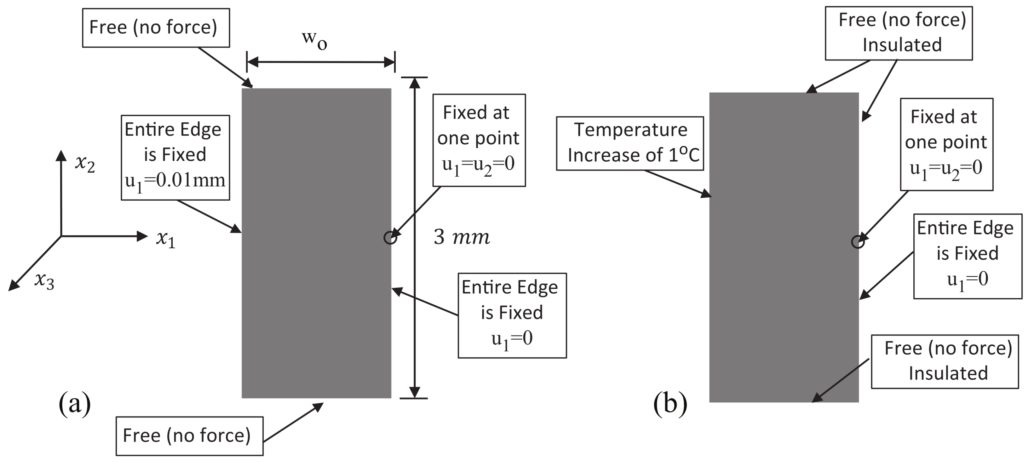
2.3. Mechanical Stiffness Tensor Predictions from Orientation

The homogenization approach for stiffness first proposed by Advani and Tucker [13] translates the constitutive behavior of the fiber and the matrix along with the spatially varying orientation distribution information to locally varying effective mechanical properties. This approach is derived in detail in [22] and was shown to extend to orthotropic reinforcement materials. The local stiffness $〈C_{ijkl}〉$ may be expressed as [13]

$$\begin{array}{c}\hfill \begin{array}{cc}〈C_{ijkl}〉=& B_1{A}_{ijkl}+B_2(A_{ij}{\delta }_{kl}+A_{kl}{\delta }_{ij})+B_3(A_{ik}{\delta }_{jl}+A_{il}{\delta }_{jk}{\delta }_{jl}+A_{jl}{\delta }_{ik}{\delta }_{jl}+A_{jk}{\delta }_{il})\hfill \\ & +B_4\left({\delta }_{ij}{\delta }_{kl}\right)+B_5({\delta }_{ik}{\delta }_{jl}+{\delta }_{il}{\delta }_{jk})\hfill \end{array}\end{array}$$

(7)

where ${\delta }_{ij}$ is the Kronecker delta, $A_{ij}$ is $\mathbf{A}$ in component form, $A_{ijkl}$ is $\mathbb{A}$ in component form, and the $B_m$ terms are given as [13]

$$\begin{array}{cc}{B}_1={\overline{C}}_{1111}+{\overline{C}}_{2222}-2{\overline{C}}_{1122}-4{\overline{C}}_{1212}\hfill & B_4={\overline{C}}_{2233}\hfill \\ B_2={\overline{C}}_{1122}-{\overline{C}}_{2233}\hfill & B_5=\frac{1}{2}({\overline{C}}_{2222}+{\overline{C}}_{2233})\hfill \\ B_3={\overline{C}}_{1212}+\frac{1}{2}({\overline{C}}_{2233}-2{\overline{C}}_{2222})\hfill \end{array}$$

(8)

where ${\overline{C}}_{ijkl}$ in Equation (8) indicates the $(i,j,k,l)$ component of the underlying unidirectional composite stiffness tensor defined in its principal material reference frame. In Equation (7), it can be seen that the material stiffness is a function of the second and the fourth-order orientation tensors as well as the underlying stiffness tensor of the unidirectional composite. The homogenization equation is constructed for dilute and semi-dilute suspensions as stress concentrations due to the fiber inclusions [13,22] are neglected. However, it was demonstrated in Caselman [50] that this approach yields reasonable results for both semi-concentrated and the low range of concentrated suspensions as well.

There are many options for the choice of micromechanics model used to calculate the unidirectional composite stiffness ${\overline{C}}_{ijkl}$ for the homogenization in Equation (7). The Halpin-Tsai micromechanics model [51], which is based on laminate theory, is a concise approach for aligned short fiber composites. However, as indicated in the work of Tucker and Liang [52], this approach is ineffective for the aspect ratios found in typical short-fiber composites, whereas the Tandon-Weng [53] and Lielens [54] models are quite effective (see e.g., [52]). Using the closed form suggested by Tucker and Liang [52], as expressed in Zhang [55], the Tandon-Weng micromechanics theory yields one of the most accurate set of solutions over the range of aspect ratios found in short-fiber composites and is used in the present study.

2.4. CTE Tensor Predictions from Orientation

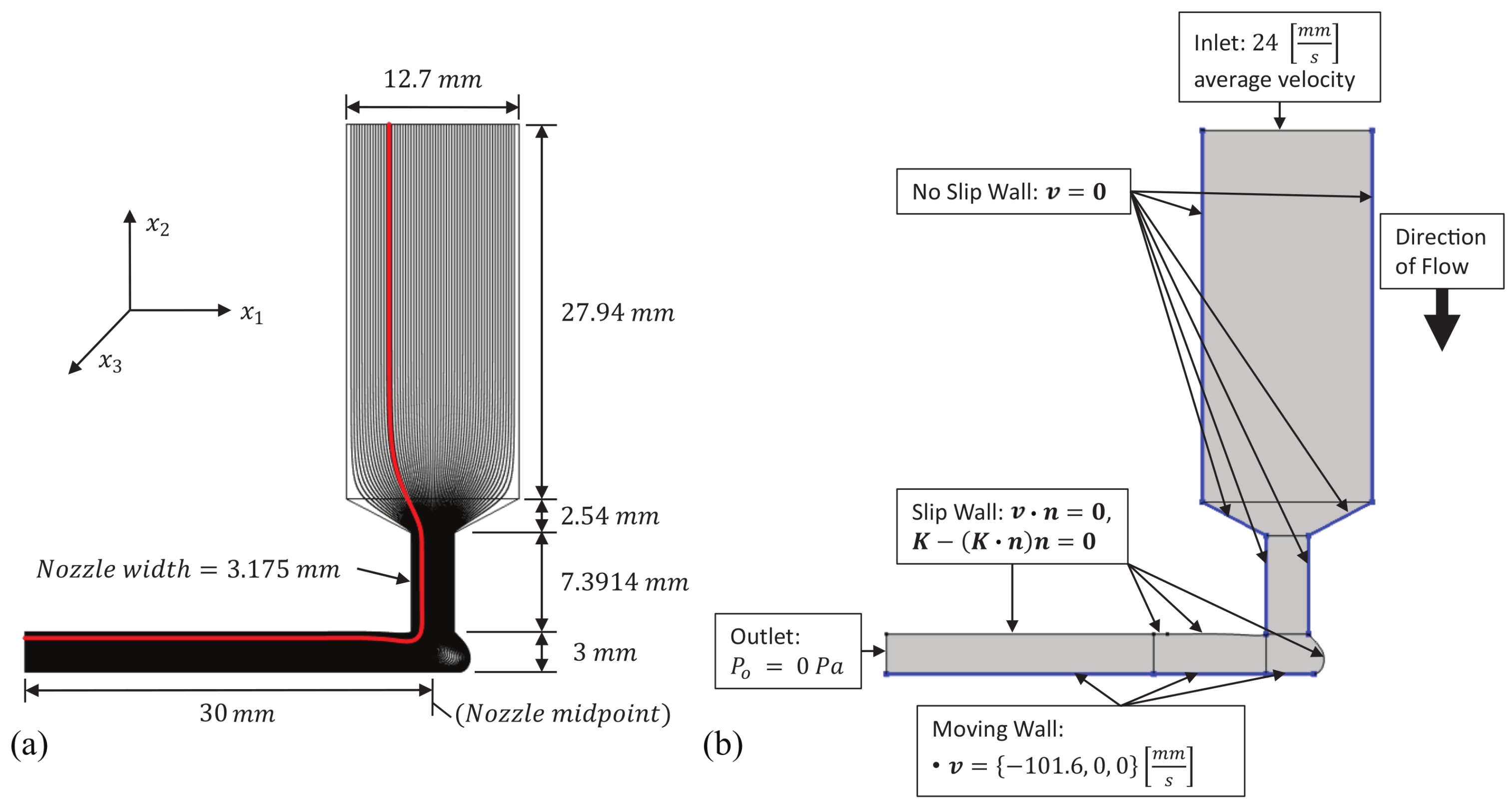
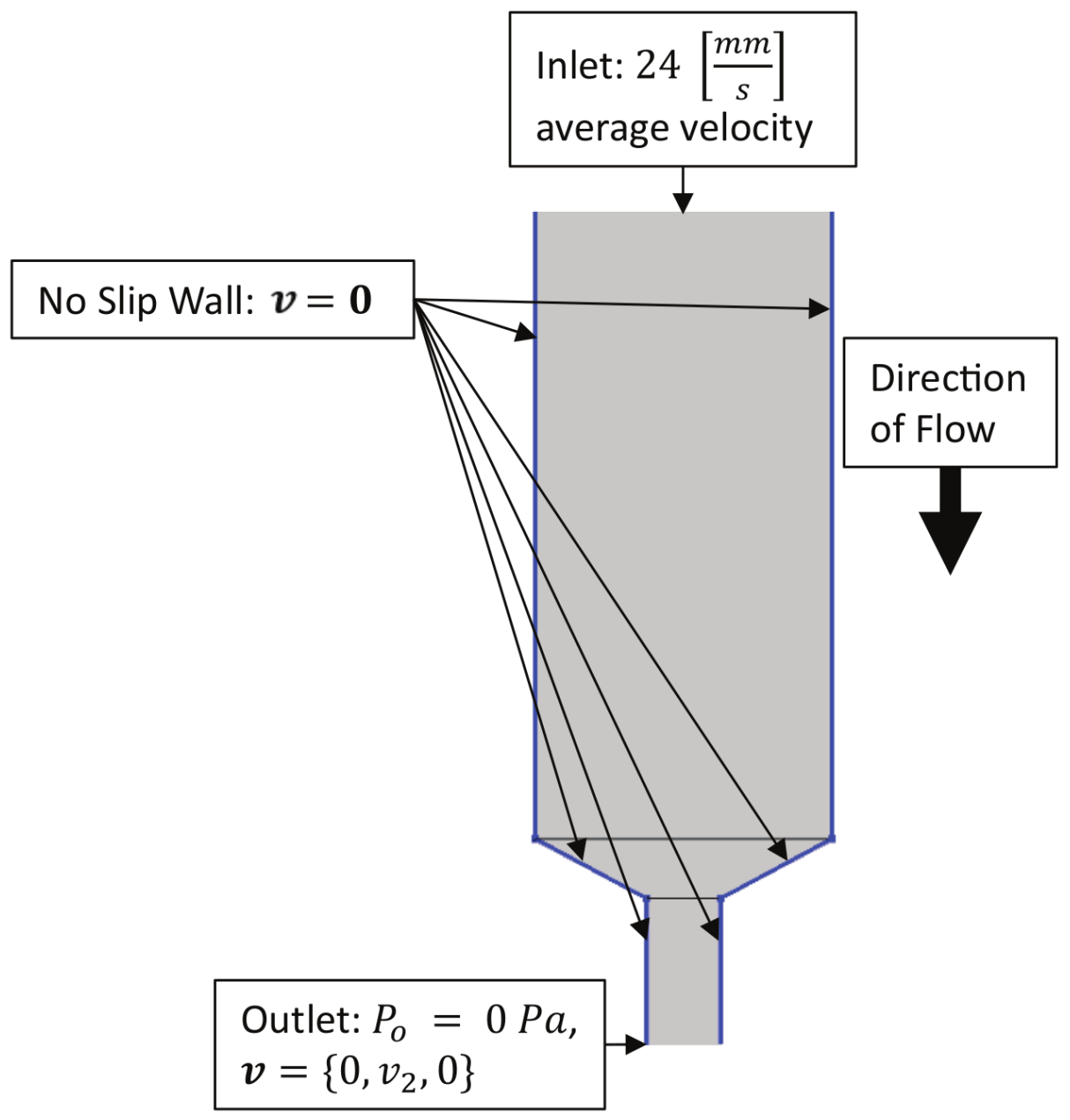
The second order, homogenized CTE tensor ${\alpha }_{ij}$ may be found from Camacho et al. [20] as

$$\begin{array}{c}\hfill 〈{\alpha }_{ij}〉=〈C_{ijkl}{\alpha }_{kl}〉{〈C_{ijkl}〉}^{-1}\end{array}$$

(9)

In this equation, ${〈C_{ijkl}〉}^{-1}$ is the inverse of $〈C_{ijkl}〉$ from Equation (7), which therefore must be determined prior to solving Equation (9). Calculating ${〈C_{ijkl}〉}^{-1}$ involves converting $〈C_{ijkl}〉$ into its contracted form, a $6\times 6$ matrix, inverting the contracted stiffness, and then converting the inverted $6\times 6$ stiffness matrix back into a full fourth order tensor. Equation (9) also involves the term $〈C_{ijkl}{\alpha }_{kl}〉$ which may be found from

$$\begin{array}{c}\hfill 〈C_{ijkl}{\alpha }_{kl}〉=D_1{A}_{ij}+D_2{\delta }_{ij}\end{array}$$

(10)

where

$$\begin{array}{c}{D}_1=A_1\left(B_1+B_2+4B_3+B_5\right)+A_2\left(B_1+3B_2+4B_3\right)\hfill \\ D_2=A_1\left(B_2+B_4\right)+A_2\left(B_2+3B_4+B_5\right)\hfill \end{array}$$

(11)

In Equation (11), the $B_i$ quantities come from Equation (8) which requires ${\overline{C}}_{ijkl}$. The $A_i$ quantities in Equation (11) come from

$$\begin{array}{ccc}\hfill A_1& =& {\alpha }_{11}-{\alpha }_{22}\hfill \\ \hfill A_2& =& {\alpha }_{22}\hfill \end{array}$$

(12)

where ${\alpha }_1$ and ${\alpha }_2$ are components of the transversely isotropic CTE tensor ${\overline{\alpha }}_{ij}$. Thus, ${\overline{\alpha }}_{ij}$ must also be predicted before Equation (9) can be calculated and this is done so using the method of Schapery [56] using the form expressed in Stair and Jack [38].

3. Flow Modeling

The planar deposition fluid flow model, defining the flow domain in this paper, is generated using the die-swell method suggested by the authors in Heller et al. [57]. A low nozzle configuration is used in this paper, where the deposited bead height is actually higher than that of the separation distance between the nozzle tip and moving platen as depicted in Figure 1a,b. The dimensions of the nozzle are taken to be similar to that of the Strangpresse Model 19 large scale FFF extrusion nozzle. The flow domain is confined within the nozzle region and experiences a no-slip boundary on the nozzle walls. Upon exiting the nozzle, the flow expands and the boundary is that of either air or the moving platen. The flow domain is modeled as a Newtonian fluid undergoing Stokes flow where the inertial effects in the flow domain are neglected as is typically done when modeling polymer flows (see e.g., [58]). The Newtonian fluid values used in the present study are those for a typical extrusion grade ABS polymer with a density, $\rho$, of 1040 kg/m${}^3$ and a dynamic viscosity, $\mu$, of 3200 Pa-s. Under the Newtonian fluid assumption, the density and viscosity only effect the pressure drop through the nozzle and do not change the velocity field within the flow domain and thus have no impact upon the resulting fiber orientation within the fluid. The modulus, CTE, and Poisson’s ratio of the ABS matrix were taken to be 2.25 GPa, $90\times {10}^{-6}$ (mm/mm)/${}^{\circ }$C, and 0.35, respectively. The Young’s modulus, CTE, Poisson’s ratio, and density of the carbon fiber were taken to be 230 GPa, $-2.6\times {10}^{-6}$ (mm/mm)/${}^{\circ }$C, 0.2, and 1700 kg/m${}^3$, respectively. The weight fraction was taken to be $13\%$ to match that of the composite system studied in Duty et al. [3] for a carbon fiber reinforced FFF bead with similar bead deposition geometry to that considered here. The shape of the fiber was taken into account using a geometric aspect ratio of 20, within the range of the carbon fiber reinforcement in [3].

The boundary conditions for the model are summarized in Figure 1b. The fiber-filled polymer enters the nozzle at the inlet with an average velocity of 24 mm/s, which would correspond to a mass flow rate of 12.2 kg/h for a circular nozzle with the same dimensions as that of the nozzle depicted in Figure 1. The nozzle walls are defined to be no-slip, meaning the velocity is zero all along the nozzle walls. The end of the bead, called the “outlet” in Figure 1b, is constrained to have zero pressure. The flat, bottom boundary of the printed bead is considered to be a moving wall with a velocity of 101.6 mm/s in the negative $x_1$ direction and zero velocity in the $x_2$ direction.

The shape of the leading and trailing free extrudate surfaces after the nozzle exit are defined using a zero surface tension minimization method presented by Heller et al. [57]. Free surfaces can be specified as zero penetration where the normal velocity is set equal to zero along the surface or zero surface tension where the normal stress along the surface is set to zero (see e.g., [59]). The selection of the curve to define the extrudate surfaces was complex due to a need for smoothness as well as having enough variability to accurately model the extrudate surface and reach an acceptable minimum. The curve that was found to give acceptable smoothness and variability for the given model is an n^th order Bezier curve ranging from 15 to 25 terms to define the polynomial, and the full details are provided in the companion paper by Heller et al. [57].

4. Results

In this section, the method of obtaining the effective longitudinal modulus and CTE is illustrated. The results between those of the full nozzle, die-swell and deposition problem are contrasted with those from a flow domain that neglects the orientational changes that occur outside of the nozzle by treating the problem as just that of an injection molded part. The flow domain of this simplified model, which is also planar, can be seen in Figure 2. The boundary conditions for the flow domain are also shown in Figure 2 and it has the same dimensions as the nozzle in the previous flow domain which was shown in Figure 1. For the new flow domain of just the nozzle, the pressure at the nozzle outlet was constrained to be 0 and the flow at the outlet was constrained to be in the normal, or vertical, direction. The flow simulations in both flow domains used an initial random orientation state, i.e., $A_{ij}=\frac{1}{3}{\delta }_{ij}$, taken to be well up-stream of the nozzle tip. In addition, the velocities and velocity gradients for both of the flow simulations were found along 61 streamlines, numbered from left to right starting from the top of the nozzle. Results are provided in this section for a comparison between the IRD and IRD-RSC models for both the full die-swell process and the flow domain that neglects the swell. After this, a final results table with the longitudinal property predictions of all the flow conditions considered will be used for conclusion purposes.

4.1. Results for a Single Flow Type—IRD, $C_I={10}^{-2}$

Beginning in COMSOL (Version 5.3; COMSOL Inc., Berlin, Germany, 2017), the flow domain was defined and the velocities in the $x_1$ and $x_2$ directions, that is $v_1$ and $v_2$, respectively, as well as the velocity gradients $\frac{\partial v_1}{\partial x_1}$, $\frac{\partial v_1}{\partial x_2}$, $\frac{\partial v_2}{\partial x_1}$, and $\frac{\partial v_2}{\partial x_2}$ were found along 61 streamlines. These were exported to MATLAB (R2016a; MathWorks, 2016) which, using an in-house implementation of the IRD model, obtained solutions for the orientation tensors for $C_I={10}^{-2}$ along each streamline. From the orientation tensors, Equations (7)–(12) were used to predict $〈C_{ijkl}〉$ and $〈{\alpha }_{ij}〉$ across cross sections of the flow domain.

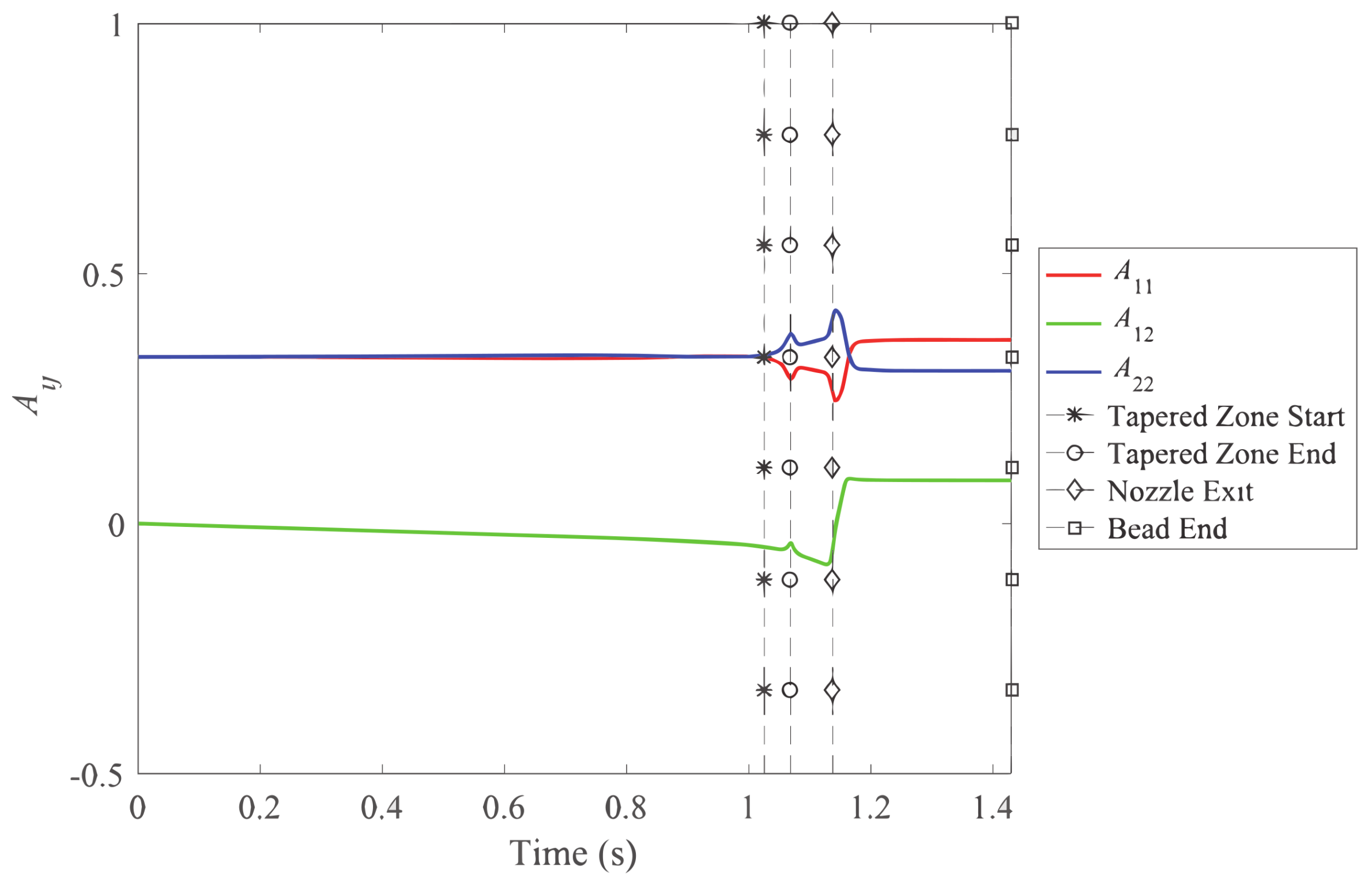
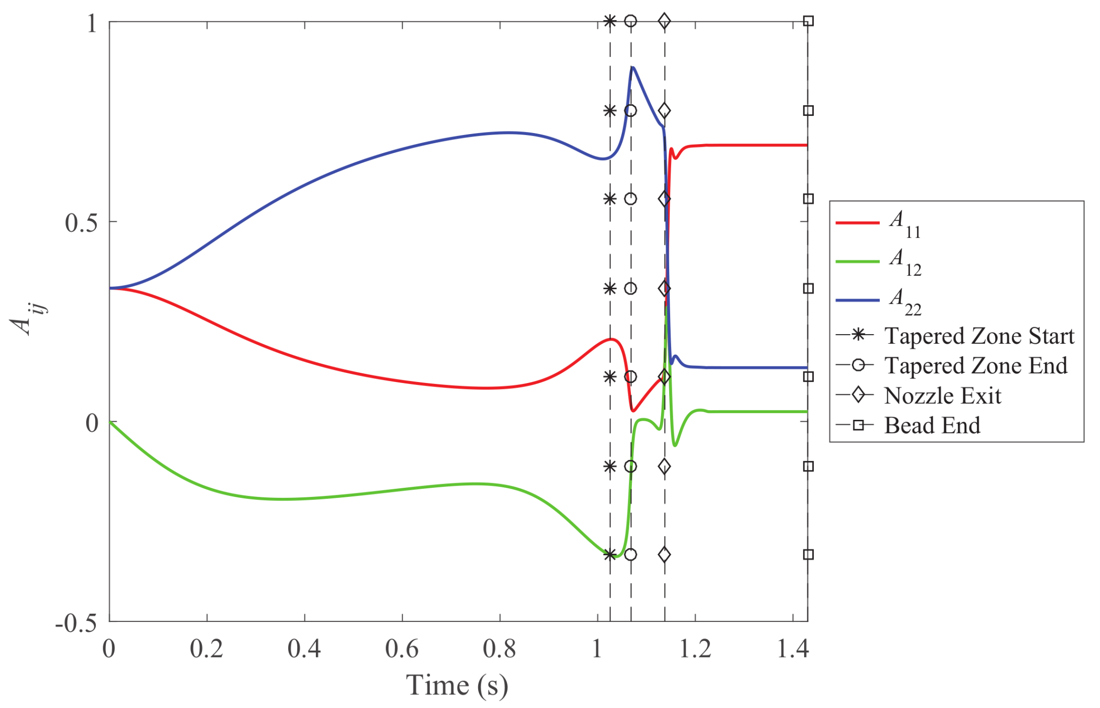
4.1.1. Orientation Tensors along a Streamline

The second order orientation tensor $A_{ij}$ was calculated using a custom code within MATLAB along streamline 15 (shown in Figure 1a) and some of the components of $A_{ij}$ are shown in Figure 3. The $A_{ij}$ results for the IRD model with $C_I={10}^{-2}$ are shown in Figure 3. It is worth noting that the choice of a random initial condition is effectively meaningless for the IRD model as the orientation attains a steady state just prior to the nozzle’s tapered zone. This will not be the case for the IRD-RSC results shown in Figure 8, where the final orientation state is clearly a function of the initial alignment state due to the slow rate of orientational changes. In the case of the IRD-RSC, a proper identification of the orientation state prior to the nozzle would need to be performed prior to industrial implementations.

There are two important cross sections of the flow that are worth highlighting. One is where the flow reaches the end of the nozzle and the other is where the flow reaches the end of the flow domain which is indicative of the final processed bead and will exhibit properties that represent the properties of the final 3D printed bead. At the end of the nozzle, the IRD model predicts a relatively high value of $A_{22}$ and a relatively low value of $A_{11}$. Since $A_{11}$ and $A_{22}$ are representative of the overall fiber alignment in the $x_1$ and $x_2$ directions, respectively, this means that the IRD model predicts that the nozzle induces a relatively high and low fiber alignment in the $x_2$ and $x_1$ directions, respectively. At the end of the flow domain, however, the IRD predicts higher $x_1$ alignment than $x_2$ alignment. Thus, the direction of highest fiber alignment tends to follow the flow direction.

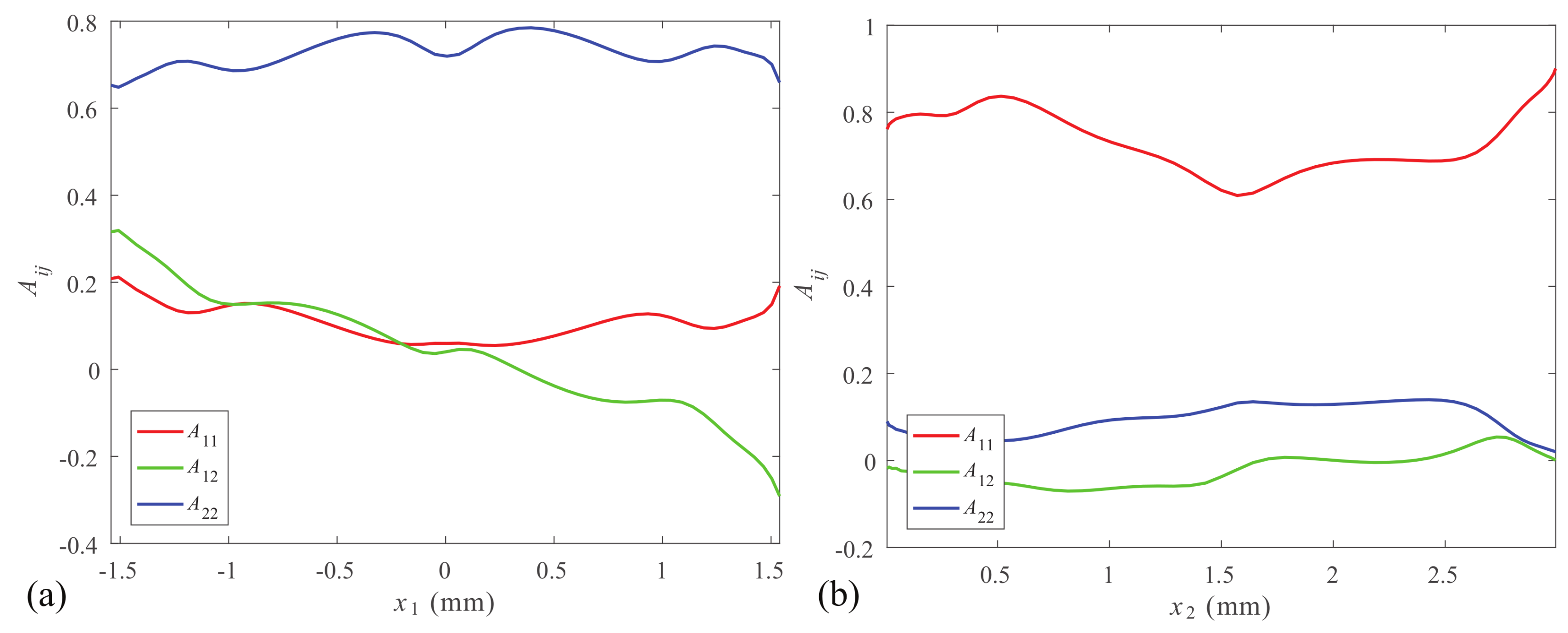
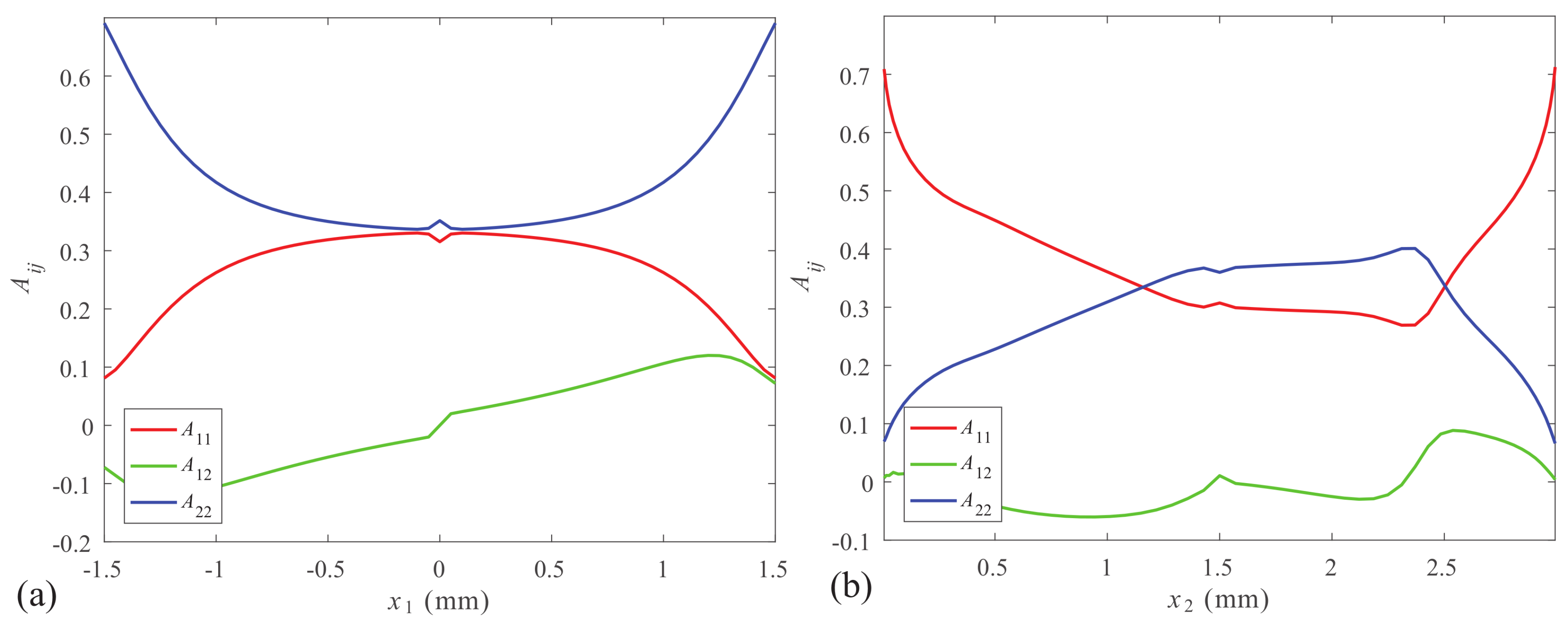
4.1.2. Orientation Tensors at the Exit and End

More information about the orientation state at the exit of the 3D printer nozzle was gained by calculating the second and fourth order orientation tensors $A_{ij}$ and $A_{ijkl}$ along 61 streamlines in the flow domain. This permitted $A_{ij}$ and $A_{ijkl}$ to be obtained across cross sections of the flow domain, such as at the nozzle exit. $A_{ij}$ as a function of $x_1$ at the nozzle exit was calculated (using the IRD model with $C_I={10}^{-2}$) and select components are shown in Figure 4a. In addition, to predict $A_{ij}$ as a function of $x_2$ at the end of the flow domain (the bead end, which is representative of the deposited bead), the flow domain as seen in Figure 1 was used. Components of $A_{ij}$ are shown in Figure 4b.

Since $A_{22}$ was found to be the dominant component of the orientation tensor along streamline 15 at the nozzle exit (see Section 4.1.1), it comes as no surprise that $A_{22}$ was the dominant component of the orientation tensor across the width of the nozzle at the nozzle exit. In addition, since the nozzle is symmetrical about the $x_2=0$ axis and the inlet condition for the flow was an average laminar inflow velocity, $A_{11}$ and $A_{22}$ are symmetrical about the $x_2=0$ axis as well and this can be seen in Figure 4a. Since $A_{12}$ contains the product of $p_1$ and $p_2$ according to Equation (2), $A_{12}$ is not symmetric about the $x_2=0$ axis. Furthermore, as $A_{11}$ was the dominant term at the end of streamline 15, it comes as no great surprise that this was the dominant $A_{ij}$ component within the deposited bead. This can be seen in Figure 4b. It can also be noted that $A_{11}$ and $A_{22}$ are not symmetrical within the deposited bead because the extruded melt turns over and experiences non-symmetrical shears as the bead is deposited.

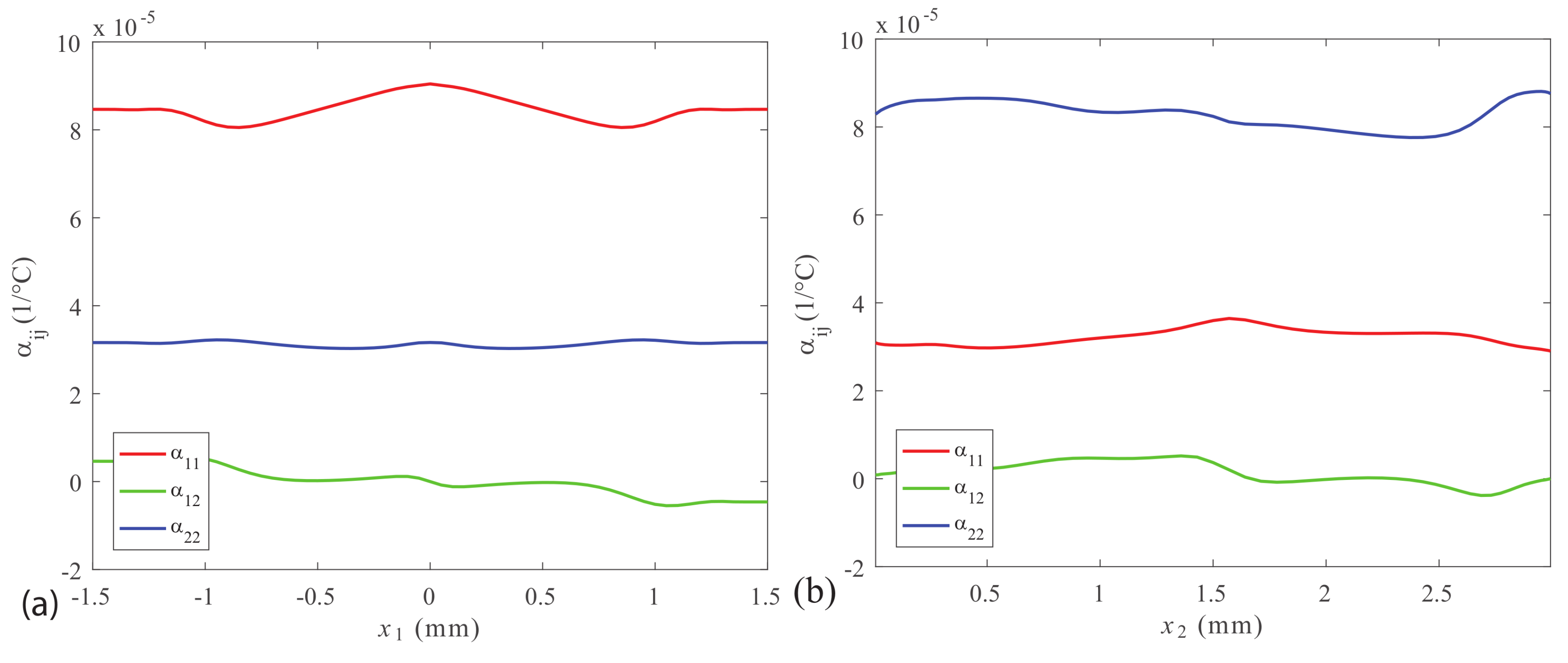
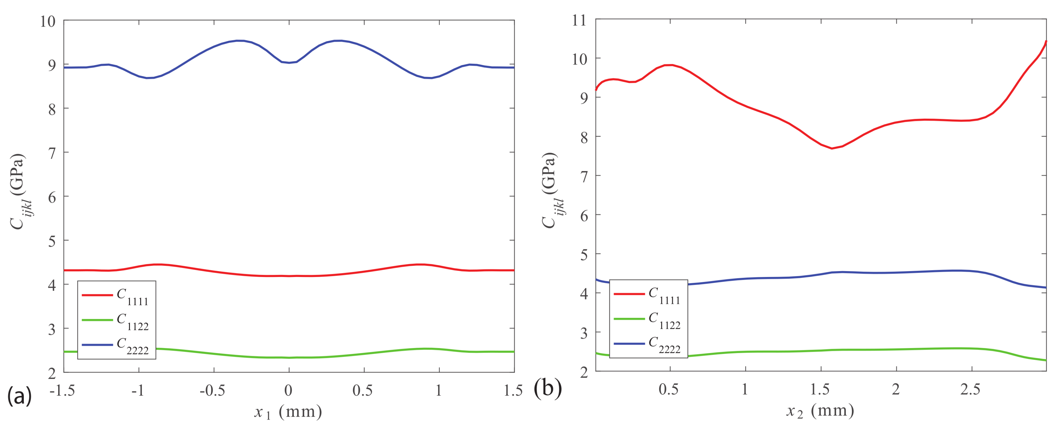
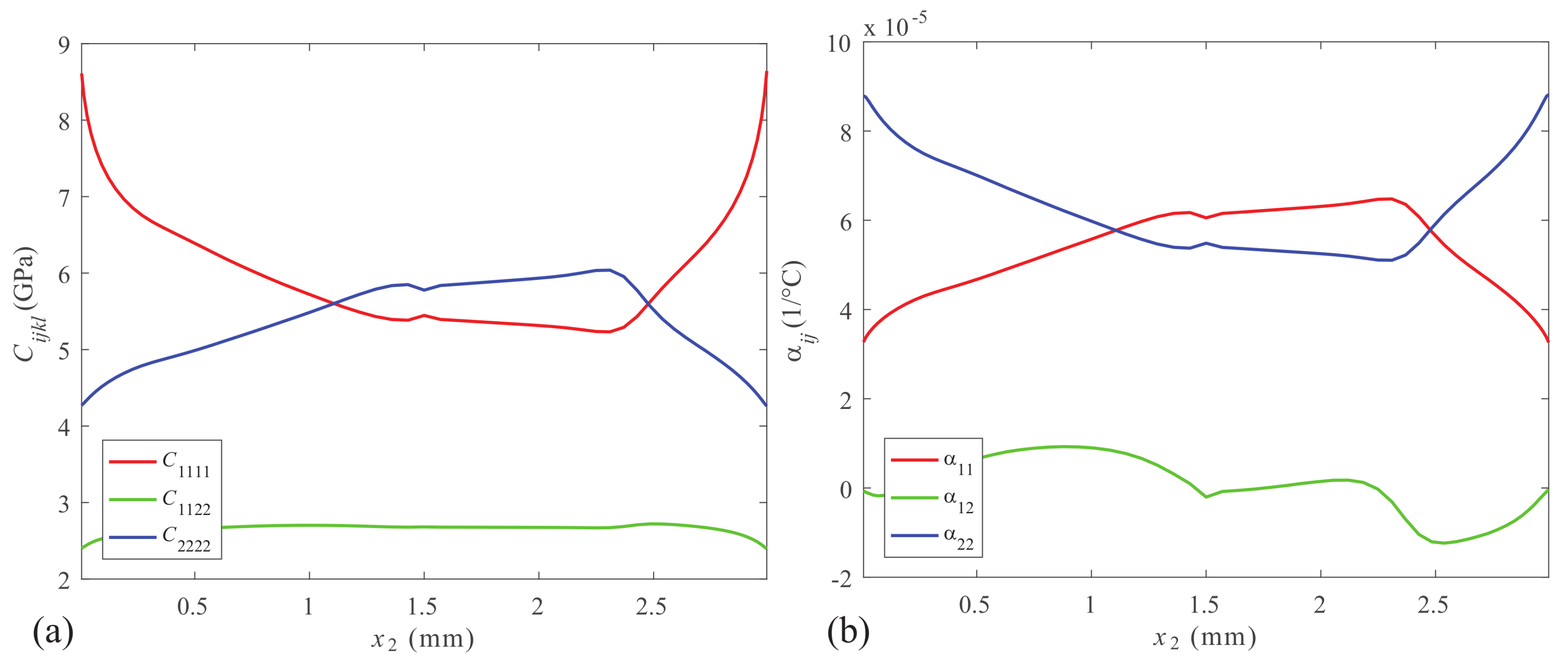
4.1.3. Stiffness and CTE at the Exit and End

In this section, we discuss the results for the stiffness and CTE at the nozzle exit and the deposited bead. Again, these results use the orientation tensors predicted using the IRD model with $C_I={10}^{-2}$, along with Equations (7)–(12). Select components of the fourth order, homogenized stiffness tensor across the nozzle exit and across the deposited bead are shown in Figure 5a,b, respectively.

There are striking similarities between Figure 4 and Figure 5. Figure 5a shows some of the components of the homogenized, fourth order stiffness tensor and shows that $〈C_{2222}〉$ dominates across the width of the nozzle at the nozzle exit. Since $〈C_{2222}〉$ is indicative of the stiffness in the $x_2$ direction, this result implies that the composite has greater stiffness in the vertical (or $x_2$) direction. It can be seen that $〈C_{2222}〉$ and $〈C_{1111}〉$ are symmetrical about $x_2=0$ at the nozzle exit and follow the trends of $A_{22}$ and $A_{11}$, respectively. Figure 5b shows similar trends to that of Figure 4b for the stiffness in the deposited bead. Again we see that $〈C_{2222}〉$ tends to follow the trend of $A_{22}$ and $〈C_{1111}〉$ follows the trend of $A_{11}$. Thus, the stiffness of the composite tends to be highest in the direction of highest fiber alignment and lower in the transverse direction. Since the direction of highest fiber alignment generally follows the direction of the flow, the direction of highest stiffness also tends to be in the flow direction.

The second order, homogenized CTE $〈{\alpha }_{ij}〉$, like $〈C_{2222}〉$, could also be found at any arbitrary point in the flow domain. Figure 6 shows some of the components of $〈{\alpha }_{ij}〉$ as a function of $x_1$ at the nozzle exit and as a function of $x_2$ within the deposited bead.

At first glance, it is perhaps harder to notice trends in the CTE that were set by the fiber orientation state, at least while using the IRD model with $C_I={10}^{-2}$. However, it can be seen that ${\alpha }_1$ is actually the dominant component of the CTE tensor at the nozzle exit and ${\alpha }_2$ is the dominant component in the deposited bead. Thus, the direction of highest fiber alignment is not the direction of highest CTE. This is due to the low CTE of carbon fibers which counteracts the higher CTE of the ABS matrix and decreases the overall CTE of the composite in the direction of highest fiber alignment. On the other hand, the direction transverse to the direction of highest fiber alignment has a relatively high CTE.

4.1.4. Effective Longitudinal Properties

After the stiffness and CTE tensors were found in the deposited bead, the stiffness tensor values were used to define the anisotropic stiffness tensor values across the width of a simulation tensile sample in COMSOL. MATLAB and COMSOL were linked via LiveLink so that the stiffness tensors, which were predicted at the end of each streamline, could be accessed by COMSOL. For COMSOL, the MATLAB function linearly interpolates the stiffness tensor values between streamlines and sets the stiffness tensor values in the region between the outermost streamlines and the boundary of the flow domain to be equivalent to the stiffness tensor values of the outermost streamlines. The simulation involved a displacement-prescribed tensile test after which the bulk, effective, longitudinal Young’s modulus was derived using the reaction stress and strain. The simulation tensile sample with boundary conditions as shown in Figure 7a represents an equivalent tensile test for obtaining the longitudinal modulus. The sample before deformation was 1.5 mm wide and 3 mm tall, the same height as the bead in Figure 1a. A $20\times 60$ rectangular element mesh was used (20 elements in $x_1$, 60 elements in $x_2$), the entire left side of the sample had a prescribed displacement of 0.01 mm in the -$x_1$ direction, the entire right side was fixed in the $x_1$ direction with the center point fixed also in the $x_2$ direction, and the top and bottom sides were free. After the displacement-prescribed tensile simulation was computed, the bulk effective longitudinal Young’s modulus in the $x_1$ direction, $E_1$, was derived using a line average method. This involved dividing the average $x_1$-reaction stress across the entire left side of the sample by the strain, where strain is the average $x_1$-displacement across the entire left side of the sample divided by the original width of the sample. In mathematical terms, this can be expressed as $E_1={\sigma }_{11}/(u_1/w_o)$, where $E_1$ is the bulk, effective, longitudinal Young’s modulus, ${\sigma }_{11}$ is the reaction stress on the left side of the sample, $u_1$ is the average displacement of the entire left side of the sample in the $x_1$ direction, and $w_o$ is the original $x_1$ dimension of the sample. Solving this equation yields a Young’s modulus at the end of the bead of $E_1$ = 6.82 GPa for the IRD model with $C_I={10}^{-2}$, not too dissimilar from those results provided in Duty et al. [3] for a similar system. A similar procedure can be done using the stiffness tensor values at the nozzle exit and this yields a Young’s modulus of $E_2$ = 7.10 GPa at the nozzle exit for the IRD model with $C_I={10}^{-2}$.

A thermomechanical analyzer (TMA) machine is often used to measure the linear CTE of a material sample by heating the sample in a furnace and measuring the displacement (expansion or contraction) of the sample along a particular direction due to the changing temperature (see, e.g., http://www.tainstruments.com/q400/). If the displacement is measured in the $x_1$ direction, for example, then the linear CTE in the $x_1$ direction can be calculated using the equation ${\alpha }_1=1/L_1\times d{L}_1/dT$, where $L_1$ is the original $x_1$-length of the sample, $d{L}_1$ is the change in the $x_1$-length, and $dT$ is the change in temperature of the sample. In this study, the boundary conditions for the representative domain for that of an equivalent test are shown in Figure 7b to calculate the bulk, effective, longitudinal CTE which is ${\alpha }_1$. The TMA sample was identical in dimensions to the tensile sample, the finite element mesh used was identical to that used in the tensile simulation, and the displacement boundary conditions were identical to those used in the tensile simulation. However, in this simulation, no loads were put on the sample. The sample was initially at a uniform temperature and a temperature increase of $\Delta T$ = 1 ${}^{\circ }$C was applied to the entire left side of the sample while the other sides were insulated. The bulk, effective, longitudinal CTE in the $x_1$ direction is calculated when thermal equilibrium is attained using the equation ${\alpha }_1=-u_1/w_o/\Delta T$, where the negative sign ensures ${\alpha }_1$ will be positive due to expansion in the $-x_1$ direction, $u_1$ is the average displacement in the $x_1$ direction of the entire left side of the sample, and $w_o$ is the initial $x_1$-length of the sample. After the TMA simulation, the bulk, effective, longitudinal CTE evaluated is ${\alpha }_1=32.2\times {10}^{-6}$/${}^{\circ }$C within the deposited bead for the IRD model with $C_I={10}^{-2}$. A similar procedure can be done for the CTE at the nozzle exit and this yields ${\alpha }_2=31.3\times {10}^{-6}$/${}^{\circ }$C at the nozzle exit for the IRD model with $C_I={10}^{-2}$.

4.2. Contrasting Results between IRD and RSC

The IRD-RSC model decreases the influence of strain on the fiber orientation state and thus predicts different values for the orientation tensors along the flow domain than the IRD model predicts and thus inevitably leads to different predictions for the stiffness and CTE tensors as well. Figure 8 shows components of $A_{ij}$ along streamline 15 in the low nozzle flow domain calculated using the IRD-RSC model with $C_I={10}^{-2}$ and $\kappa =1/30$. The IRD-RSC model predicted a much lower rate of alignment than the IRD model (compare Figure 8 with Figure 3), although the IRD-RSC model predicted a similar trend in the changes in the components of $A_{ij}$ along streamline 15. That is, $A_{22}$ is highest at the nozzle exit but $A_{11}$ is highest at the bead end, indicating that the fibers tend to align most in the flow direction.

Components of $A_{ij}$ across the nozzle exit and within the deposited bead, calculated using the IRD-RSC model with $C_I={10}^{-2}$ and $\kappa =1/30$, are shown in Figure 9. Once again, $A_{11}$ and $A_{22}$ are symmetrical about the $x_2=0$ axis at the nozzle exit as one would expect. Figure 9a shows that the IRD-RSC model predicts much higher $x_2$ alignment along the sides of the nozzle. This is due to the higher shear along the sides of the nozzle. Figure 9b also shows that the fiber alignment is highest near the sides of the flow domain in the deposited bead.

The homogenized stiffness and CTE tensors were also calculated using the orientation tensors from the IRD-RSC model with $C_I={10}^{-2}$ and $\kappa =1/30$. The results for these quantities at the end of the bead for the low nozzle domain are shown in Figure 10. Once again, it can be seen that the stiffness tends to follow a similar trend as the orientation tensors and that the CTE, in a sense, follows the opposite trend. Regardless, when comparing the results from that of the IRD-RSC with $\kappa =1/30$ to that of the IRD model with the same interaction coefficient $C_I$, there is a clear difference in the orientation, the stiffness, and the resulting coefficient of thermal expansion. Performing the same finite element analysis as in the preceding section within the deposited bead, the bulk longitudinal stiffness is $E_1$ = 4.82 GPa and the bulk coefficient of thermal expansion is ${\alpha }_1=45.5\times {10}^{-6}$/${}^{\circ }$C. Both of these numbers are significantly different than those of the IRD results.

4.3. Effective Longitudinal Properties—All Flow Conditions

Using the methodology discussed above, the effective, longitudinal stiffness and CTE properties are studied as functions of the interaction model, the degree of fiber interaction $C_I$, the amount of slowness $\kappa$, and whether or not the die swell is included in the analysis. A fiber interaction coefficient of $C_I=3\times {10}^{-3}$ is chosen to represent melt with a lower degree of interaction, and slowness parameters of $\kappa =1/10$ and $1/30$ are presented.

Table 1. Summary of Effective Longitudinal Properties for All Flow Conditions.

Location	Model	${\mathit{C}}_{\mathit{I}}$	$\mathit{\kappa }$	${\mathit{E}}_{\mathbf{long}}$ (GPa)	${\mathit{\alpha }}_{\mathbf{long}}\times {10}^{-6}$/${}^{\circ }$C
Deposited Bead	IRD	0.01	1	6.82	32.2
Deposited Bead	RSC	0.01	1/10	4.82	45.5
Deposited Bead	RSC	0.01	1/30	4.18	53.3
Deposited Bead	IRD	0.003	1	7.69	30.3
Deposited Bead	RSC	0.003	1/10	4.88	45.1
Deposited Bead	RSC	0.003	1/30	4.19	53.2
Nozzle Exit	IRD	0.01	1	7.10	31.3
Nozzle Exit	RSC	0.01	1/10	5.07	42.4
Nozzle Exit	RSC	0.01	1/30	4.40	49.5
Nozzle Exit	IRD	0.003	1	7.89	29.9
Nozzle Exit	RSC	0.003	1/10	5.20	41.7
Nozzle Exit	RSC	0.003	1/30	4.45	49.2

shows the results from the complete study. Comparisons of the results of the deterministic models between the various parameters is made through the use of the percent relative difference, defined as

$$\begin{array}{c}\hfill PRD=\left(\right|valu{e}_1-valu{e}_2\left|\right)/\left(\right|valu{e}_1-valu{e}_2|/2)\times 100\%\end{array}$$

(13)

The first study is of the relative importance of the full die-swell model and bead deposition versus that of model domain that stops at the nozzle end. Taking the bulk stiffness and CTE results from the IRD model, the PRD for the longitudinal modulus $E_{long}$ would be 4.02% for $C_I={10}^{-2}$ and 2.56% for $C_I=3\times {10}^{-3}$, whereas for the same interaction coefficients and a $\kappa =1/10$ the PRD in the longitudinal modulus is respectively, 5.05% and 6.34% with similar percentages for a $\kappa =1/30$. The trend in the PRD in the various CTEs ranges between 1.3% and 7.8%. Thus, it would appear that if the ultimate objective is the bulk behavior of the composite, the inclusion of the full model domain with die swell and deposition on the moving platen will refine the results on the order of 5%.

Focusing on the results from the deposited bead and looking at the results as a function of the interaction coefficient for the IRD model, there is a 12% PRD for the longitudinal modulus and a 6% PRD for the longitudinal CTE as the interaction coefficient changes from $C_I=3\times {10}^{-3}$ to ${10}^{-2}$. The change as a function of interaction coefficient is nearly non-existent when the IRD-RSC model is used with either value of $\kappa$, with the greatest PRD of 1.3% occurring in the longitudinal modulus for $\kappa =1/10$.

Comparing the results of the IRD model to that of the IRD-RSC model with $\kappa =1/10$, the PRD in the longitudinal modulus for $C_I={10}^{-2}$ is 34% and for $C_I=3\times {10}^{-3}$ it is nearly 45%, with similar numbers for the CTE values. Similarly, when looking at the longitudinal modulus for $\kappa =1/10$ as compared to that of $\kappa =1/30$, the PRD is 14% for the higher $C_I$ and 15% for the lower $C_I$, with similar values for the PRD of the CTEs.

Thus, of all the comparisons, the results are most sensitive to the choice of whether or not to use the IRD-RSC model or the original IRD model. It is very interesting to note, that in this flow scenario, where the melt experiences a rapid change in the nozzle region and then the velocity gradients go to zero, the choice of the interaction coefficient has very little bearing on the final part behavior for the newer IRD-RSC model. This observation is in contrast to results within an injection molded product as there is a large period of the melt time that the fibers are subjected to a shear after they have left the mold inlet. It is also worth noting, that although the die-swell and deposition have a substantial bearing on the internal orientation state, the bulk material response is less sensitive to that effect than to issues effecting the interaction coefficient and the slowness parameter. It would also be appropriate to note the sensitivity of the choice of initial conditions on the orientation tensor for the IRD-RSC model. The initial condition can be neglected for the IRD model as the orientation reaches a steady state prior to the tapered nozzle region, but for the IRD-RSC results this is not the case and the final orientation maintains some history based on the somewhat arbitrary choice of the initial conditions.

5. Conclusions

In this study, we have developed a methodology for predicting the fiber orientation state within the flow of an FFF 3D printer and subsequently predicting the effective, longitudinal stiffness $E_{\mathrm{long}}$ and CTE ${\alpha }_{\mathrm{long}}$. We found that incorporating the die swell into the FFF flow domain did not have a substantial impact on the predicted moduli. However, there was a significant difference between the IRD predictions and the IRD-RSC predictions. When the interaction coefficient $C_I$ varies within the range 0.003–0.01, it has moderate effects on the IRD predictions but the effects are insignificant on the IRD-RSC predictions. Finally, varying the value of the slowness factor $\kappa$, which appears in the IRD-RSC model, does indeed appear to significantly affect the $E_{\mathrm{long}}$ and ${\alpha }_{\mathrm{long}}$ predictions. A future study will focus on experimental validation of the computational methodology used in this paper.

References

1. Kannan, S.; Senthilkumaran, D.; Elangovan, K. Development of Composite Materials by Rapid Prototyping Technology using FDM Method. In Proceedings of the IEEE International Conference on Current Trends in Engineering and Technology (ICCTET), Coimbatore, India, 3 July 2013; pp. 281–283. [Google Scholar]
2. Lind, R.; Post, B.; Blue, C.; Love, L. Enhanced Additive Manufacturing with a Reciprocating Leveling and Force Sensing Platen; Technical Report 201403257; Oak Ridge National Laboratory: Oak Ridge, TN, USA, 2014.
3. Duty, C.; Kunc, V.; Compton, B.; Post, B.; Erdman, D.; Smith, R.; Lind, R.; Lloyd, P.; Love, L. Structure and Mechanical Behavior of Big Area Additive Manufacturing (BAAM) Materials. Rapid Prototyp. J. 2017, 23, 181–189. [Google Scholar] [CrossRef]
4. Kishore, V.; Ajinjeru, C.; Nycz, A.; Post, B.; Lindahl, J.; Kunc, V.; Duty, C. Infrared preheating to improve interlayer strength of big area additive manufacturing (BAAM) components. Addit. Manuf. 2017, 14, 7–12. [Google Scholar] [CrossRef]
5. Narahara, H.; Shirahama, Y.; Koresawa, H. Improvement and Evaluation of the Interlaminar Bonding Strength of FDM Parts by Atmospheric-Pressure Plasma. Proc. CIRP 2016, 42, 754–759. [Google Scholar] [CrossRef]
6. Lau, K.; Hung, P.; Zhu, M.; Hui, D. Properties of natural fibre composites for structural engineering applications. Compos. Part B Eng. 2018, 136, 222–233. [Google Scholar] [CrossRef]
7. Soutis, C. Fibre reinforced composites in aircraft construction. Prog. Aerosp. Sci. 2015, 41, 143–151. [Google Scholar] [CrossRef]
8. Sfondrini, M.; Cacciafesta, V.; Scribante, A. Shear bond strength of fibre-reinforced composite nets using two different adhesive systems. Eur. J. Orthod. 2011, 33, 66–70. [Google Scholar] [CrossRef] [PubMed]
9. Cacciafesta, V.; Sfondrini, M.; Lena, A.; Scribante, A.; Vallittu, P.; Lassila, L. Flexural strengths of fiber-reinforced composites polymerized with conventional light-curing and additional postcuring. Am. J. Orthodont. Dent. Orthop. 2007, 132, 524–527. [Google Scholar] [CrossRef] [PubMed]
10. Love, L.; Kunk, V.; Rios, O.; Duty, C.; Elliott, A.; Post, B.; Smith, R.; Blue, C. The Importance of Carbon Fiber to Polymer Additive Manufacturing. J. Mater. Res. 2014, 29, 1893–1898. [Google Scholar] [CrossRef]
11. Tekinalp, H.; Kunc, V.; Velez-Garcia, G.; Duty, C.; Love, L.; Naskar, A.; Blue, C.; Ozcan, S. Highly Oriented Carbon Fiber-Polymer Composites via Additive Manufacturing. Compos. Sci. Technol. 2014, 105, 144–150. [Google Scholar] [CrossRef]
12. Folgar, F.; Tucker, C. Orientation Behavior of Fibers in Concentrated Suspensions. J. Reinf. Plast. Compos. 1984, 3, 98–119. [Google Scholar] [CrossRef]
13. Advani, S.G.; Tucker, C. The Use of Tensors to Describe and Predict Fiber Orientation in Short Fiber Composites. J. Rheol. 1987, 31, 751–784. [Google Scholar] [CrossRef]
14. Cintra, J.S.; Tucker, C. Orthotropic Closure Approximations for Flow-Induced Fiber Orientation. J. Rheol. 1995, 39, 1095–1122. [Google Scholar] [CrossRef]
15. Koch, D. A Model for Orientational Diffusion in Fiber Suspensions. Phys. Fluids 1995, 7, 2086–2088. [Google Scholar] [CrossRef]
16. Huynh, H.M. Improved Fiber Orientation Predictions for Injection-Molded Composites. Master’s Thesis, University of Illinois at Urbana-Champaign, Champaign, IL, USA, 2001. [Google Scholar]
17. Wang, J.; O’Gara, J.; Tucker, C. An Objective Model for Slow Orientation Kinetics in Concentrated Fiber Suspensions: Theory and Rheological Evidence. J. Rheol. 2008, 52, 1179–1200. [Google Scholar] [CrossRef]
18. Phelps, J.; Tucker, C. An Anisotropic Rotary Diffusion Model for Fiber Orienation in Short- and Long Fiber Thermoplastics. J. Non-Newt. Fluid Mech. 2009, 156, 165–176. [Google Scholar] [CrossRef]
19. Ortman, K.; Baird, D. Using Startup of Steady Shear Flow in a Sliding Plate Rheometer to Determine Material Parameters for the Purpose of Predicting Long Fiber Orientation. J. Rheol. 2012, 56, 955–981. [Google Scholar] [CrossRef]
20. Camacho, C.; Tucker, C.; Yalvac, S.; McGee, R. Stiffness and Thermal Expansion Predictions for Hybird Short Fiber Composites. Polym. Compos. 1990, 11, 229–239. [Google Scholar] [CrossRef]
21. Gusev, A.; Heggli, M.; Lusti, H.; Hine, P. Orientation Averaging for Stiffness and Thermal Expansion of Short Fiber Composites. Adv. Eng. Mater. 2002, 4, 931–933. [Google Scholar] [CrossRef]
22. Jack, D.; Smith, D. Elastic Properties of Short-Fiber Polymer Composites, Derivation and Demonstration of Analytical Forms for Expectation and Variance from Orientation Tensors. J. Compos. Mater. 2008, 42, 277–308. [Google Scholar] [CrossRef]
23. Jeffery, G. The Motion of Ellipsoidal Particles Immersed in a Viscous Fluid. Proc. R. Soc. Lond. A 1923, 102, 161–179. [Google Scholar] [CrossRef]
24. Bay, R.; Tucker, C. Fiber orientation in simple injection moldings. Part I: Theory and numerical methods. Polym. Compos. 1992, 13, 317–331. [Google Scholar] [CrossRef]
25. Montgomery-Smith, S.J.; Jack, D.; Smith, D. A Systematic Approach to Obtaining Numerical Solutions of Jeffery’s Type Equations using Spherical Harmonics. Compos. Part A 2010, 41, 827–835. [Google Scholar] [CrossRef]
26. Dinh, S.; Armstrong, R. A Rheological Equation of State for Semiconcentrated Fiber Suspensions. J. Rheol. 1984, 28, 207–227. [Google Scholar] [CrossRef]
27. Lipscomb, G.I.; Denn, M.; Hur, D.; Boger, D. Flow of Fiber Suspensions in Complex Geometries. J. Non-Newt. Fluid Mech. 1988, 26, 297–325. [Google Scholar] [CrossRef]
28. Verweyst, B.; Tucker, C.L., III. Fiber Suspensions in Complex Geometries: Flow-Orientation Coupling. Can. J. Chem. Eng. 2002, 80, 1093–1106. [Google Scholar] [CrossRef]
29. Chung, D.; Kwon, T. Numerical Studies of Fiber Suspensions in an Axisymmetric Radial Diverging Flow: The Effects of Modeling and Numerical Assumptions. J. Non-Newt. Fluid Mech. 2002, 107, 67–96. [Google Scholar] [CrossRef]
30. Advani, S.; Tucker, C. Closure Approximations for Three-Dimensional Structure Tensors. J. Rheol. 1990, 34, 367–386. [Google Scholar] [CrossRef]
31. Nguyen, N.; Bapanapalli, S.; Kunc, V.; Phelps, J.; Tucker, C. Prediction of the Elastic-Plastic Stress/Strain Response for Injection-Molded Long-Fiber Thermoplastics. J. Compos. Mater. 2009, 43, 217–246. [Google Scholar] [CrossRef]
32. Bird, R.B.; Curtiss, C.; Armstrong, R.C.; Hassager, O. Dynamics of Polymeric Liquids. Vol. 2: Kinetic Theory, 2nd ed.; John Wiley & Sons, Inc.: New York, NY, USA, 1987. [Google Scholar]
33. Phan-Thien, N.; Fan, X.J.; Tanner, R.; Zheng, R. Folgar-Tucker Constant for a Fibre Suspension in a Newtonian Fluid. J. Non-Newt. Fluid Mech. 2002, 103, 251–260. [Google Scholar] [CrossRef]
34. Sepehr, M.; Carreau, P.; Grmela, M.; Ausias, G.; Lafleur, P. Comparison of Rheological Properties of Fiber Suspensions with Model Predictions. J. Polym. Eng. 2004, 24, 579–610. [Google Scholar] [CrossRef]
35. Strautins, U.; Latz, A. Flow-Driven Orientation Dynamics of Semiflexible Fiber Systems. Rheol. Acta 2007, 46, 1057–1064. [Google Scholar] [CrossRef]
36. Nguyen, N.; Bapanapalli, S.; Holbery, J.; Smith, M.; Kunc, V.; Frame, B.; Phelps, J.; Tucker, C. Fiber Length and orientation in Long-Fiber Injection-Molded Thermoplastics—Part I: Modeling of Microstructure and Elastic Properties. J. Compos. Mater. 2008, 42, 1003–1029. [Google Scholar] [CrossRef]
37. Agboola, B.; Jack, D.; Montgomery-Smith, S. Effectiveness of Recent Fiber-interaction Diffusion Models for Orientation and the Part Stiffness Predictions in Injection Molded Short-fiber Reinforced Composites. Compos. Part A 2012, 43, 1959–1970. [Google Scholar] [CrossRef]
38. Stair, S.; Jack, D. Comparison of Experimental and Modeling Results for Cure Induced Curvature of a Carbon Fiber Laminate. Polym. Compos. 2017, 38, 2488–2500. [Google Scholar] [CrossRef]
39. Zhang, D.; Smith, D.; Jack, D.; Montgomery-Smith, S. Numerical Evaluation of Single Fiber Motion for Short-Fiber-Reinforced Composite Materials Processing. J. Manuf. Sci. Eng. 2011, 133, 051002. [Google Scholar] [CrossRef]
40. Doi, M. Molecular Dynamics and Rheological Properties of Concentrated Solutions of Rodlike Polymers in Isotropic and Liquid Crystalline Phases. J. Polym. Sci. Part B Polym. Phys. 1981, 19, 229–243. [Google Scholar] [CrossRef]
41. Hand, G. A Theory of Anisotropic Fluids. J. Fluid Mech. 1962, 13, 33–46. [Google Scholar] [CrossRef]
42. Chung, D.; Kwon, T. Improved Model of Orthotropic Closure Approximation for Flow Induced Fiber Orientation. Polym. Compos. 2001, 22, 636–649. [Google Scholar] [CrossRef]
43. Chung, D.; Kwon, T. Invariant-Based Optimal Fitting Closure Approx. for the Numerical Prediction of Flow-Induced Fiber Orientation. J. Rheol. 2002, 46, 169–194. [Google Scholar] [CrossRef]
44. Jack, D.; Schache, B.; Smith, D. Neural Network Based Closure for Modeling Short-Fiber Suspensions. Polym. Compos. 2010, 31, 1125–1141. [Google Scholar] [CrossRef]
45. Montgomery-Smith, S.J.; Jack, D.; Smith, D. The Fast Exact Closure for Jeffery’s Equation with Diffusion. J. Non-Newt. Fluid Mech. 2011, 166, 343–353. [Google Scholar] [CrossRef]
46. Montgomery-Smith, S.J.; He, W.; Jack, D.; Smith, D. Exact Tensor Closures for the Three Dimensional Jeffery’s Equation. J. Fluid Mech. 2011, 680, 321–335. [Google Scholar] [CrossRef]
47. Jack, D.; Smith, D. An Invariant Based Fitted Closure of the Sixth-order Orientation Tensor for Modeling Short-Fiber Suspensions. J. Rheol. 2005, 49, 1091–1116. [Google Scholar] [CrossRef]
48. Jack, D.; Smith, D. Sixth-order Fitted Closures for Short-fiber Reinforced Polymer Composites. J. Thermoplast. Compos. 2006, 19, 217–246. [Google Scholar] [CrossRef]
49. Velez-Garcia, G.; Mazahir, S.; Hofmann, J.; Wapperom, P.; Barid, D.; Zink-Sharp, A.; Kunc, V. Improvement in Orientation Measurement for Short and Long Fiber Injection Molded Composites. In Proceedings of the 10th Annual SPE Automotive Composites Conference and Exposition, Detroit, MI, USA, 15–16 September 2010. [Google Scholar]
50. Caselman, E. Elastic Property Prediction of Short Fiber Composites Using a Uniform Mesh Finite Element Method. Master’s Thesis, University of Missouri, Columbia, MO, USA, 2007. [Google Scholar]
51. Halpin, J. Stiffness and Expansion Estimates for Oriented Short Fiber Composites. J. Compos. Mater. 1969, 3, 732–734. [Google Scholar] [CrossRef]
52. Tucker, C.; Liang, E. Stiffness Predictions for Unidirectional Short-Fiber Composites: Review and Evaluation. Compos. Sci. Technol. 1999, 59, 655–671. [Google Scholar] [CrossRef]
53. Tandon, G.; Weng, G. The Effect of Aspect Ratio of Inclusions on the Elastic Properties of Unidirectionally Aligned Composites. Polym. Compos. 1984, 5, 327–333. [Google Scholar] [CrossRef]
54. Lielens, G.; Pirotte, P.; Couniot, A.; Dupret, F.; Keunings, R. Prediction of Thermo-Mech Properties for Compression Moulded Composites. Compos. Part A 1998, 29, 63–70. [Google Scholar] [CrossRef]
55. Zhang, C. Modeling of Flexible Fiber Motion and Prediction of Material Properties. Master’s Thesis, Baylor University, Waco, TX, USA, 2011. [Google Scholar]
56. Schapery, R. Thermal Expansion Coefficients of Composite Materials Based on Energy Principles. J. Compos. Mater. 1968, 2, 380–404. [Google Scholar] [CrossRef]
57. Heller, B.; Smith, D.; Jack, D. Simulation of Planar Deposition Polymer Melt Flow and Fiber Orientation in Fused Filament Fabrication. In Proceedings of the Solid Freeform Fabrication Symposium, Austin, TX, USA, 7–9 August 2017; pp. 1096–1111. [Google Scholar]
58. Tadmor, Z.; Gogos, C. Principles of Polymer Processing, 2nd ed.; Wiley Interscience: Hoboken, NJ, USA, 2006. [Google Scholar]
59. Athanasopulos, I.; Makrakis, G.; Rodrigues, J.F. Free Boundary Problems: Theory and Applications; Chapman and Hill/CRC Press: Boca Raton, FL, USA, 1999. [Google Scholar]
Figure 1. (a) The flow domain and dimensions; streamline 15 is highlighted in red. (b) The flow domain with boundary conditions.
Jcs 02 00026 g001
Figure 2. The flow domain of the nozzle alone with boundary conditions. (Nozzle dimensions are the same as those shown in Figure 1).
Jcs 02 00026 g002
Figure 3. Components of A i j , predicted with the IRD model with C I = 10 2 , along streamline 15.
Jcs 02 00026 g003
Figure 4. Orientation tensors calculated using the IRD model with C I = 10 2 . (a) A i j as a function of x 1 at the nozzle exit, calculated using the model in Figure 2, and (b) A i j as a function of x 2 within the deposited bead, calculated using the model in Figure 1.
Jcs 02 00026 g004
Figure 5. Components of C i j k l from using the IRD model with C I = 10 2 (a) as a function of x 1 at the nozzle exit, and (b) as a function of x 2 within the deposited bead.
Jcs 02 00026 g005
Figure 6. Components of α i j from using the IRD model with C I = 10 2 (a) as a function of x 1 at the nozzle exit, and (b) as a function of x 2 at the end of the bead.
Jcs 02 00026 g006
Figure 7. Boundary conditions for finite element analysis: (a) the tensile sample boundary conditions, and (b) the TMA boundary conditions.
Jcs 02 00026 g007
Figure 8. A i j components along streamline 15—results are from using the IRD-RSC model with C I = 10 2 and κ = 1 / 30 .
Jcs 02 00026 g008
Figure 9. Orientation tensors calculated from the IRD-RSC model with C I = 10 2 and κ = 1 / 30 . (a) A i j as a function of x 1 at the nozzle exit and (b) A i j as a function of x 2 within the deposited bead.
Jcs 02 00026 g009
Figure 10. Results in the deposited bead from the IRD-RSC model with C I = 10 2 and κ = 1 / 30 . (a) C i j k l as a function of x 2 in the deposited bead, and (b) α i j as a function of x 2 .
Jcs 02 00026 g010