Numerical Study of the Mixed-Mode Delamination of Composite Specimens


1
Department of Innovation Engineering, University of Salento, Lecce 73100, Italy
2
Department of Civil, Chemical, Environmental and Materials Engineering (DICAM), School of Engineering and Architecture, University of Bologna, Bologna 40136, Italy
*
Author to whom correspondence should be addressed.
J. Compos. Sci. 2018, 2(2), 30; https://doi.org/10.3390/jcs2020030
Submission received: 15 April 2018
/
Revised: 30 April 2018
/
Accepted: 2 May 2018
/
Published: 4 May 2018
(This article belongs to the Special Issue Mechanics of Innovative Materials in Engineering Applications)
Abstract
:The present research deals with the delamination process in multi-layered composite specimens, with a reduced computational effort. The adhesive interface between sublaminates is represented as a continuous distribution of elastic-brittle springs in the normal and/or tangential direction depending on the interfacial mixed-mode condition. Each composite adherend, instead, is modelled according to the Timoshenko’s beam theory. The proposed formulation is here enhanced through the Generalized Differential Quadrature (GDQ) method, where the differential equations of the problem are solved directly in a strong form. Thus, the possibility of tracking the delamination response of the specimens is provided locally in a numerical sense, in terms of interface stresses, internal forces and displacements but also in terms of critical fracture energies and mode mixity angles. A further check of the proposed formulation is performed with respect to some standard solutions available in literature. The good agreement between numerical and theoretical predictions verifies the efficiency of the proposed GDQ approach for the study of complex mixed-mode delamination phenomena in composite materials and joints.
1. Introduction
In a context where a lot of engineering components and material systems are layered and made of high performance composites, an increased attention in the last decades has focused on the development of appropriate numerical tools to simulate the complex damage process known as delamination. This phenomenon can be approached at different scales, from the microscale up to the macroscale. At the micro-level, indeed, the cracks form within the matrix-reach regions, affecting the interfacial weakness of the microstructure. At a macro-level, laminated models are appropriate when the structure is subjected to in-plane, bending or combined loading conditions, as considered in the parametric analysis of the present work.
Different methods based on strength of materials or on fracture mechanics are applied in literature to detect the onset of damage, according to experimental observations, as well as to analytical or numerical approaches. In the first case, several test configurations have been developed to measure the delamination strength and/or toughness, see for example, [1,2,3,4], among others. The mixed-mode delamination can either be modelled through analytical approaches, accounting for possible geometrical and mechanical non-linearities of materials and interfaces.
In the pioneering work by Williams [5], the beam theory was applied to determine the mixed-mode energy release rate and its pure-mode contributions and , for homogeneous beams with arbitrary crack depths. Suo and Hutchinson proposed a Local Method (LM) to determine the mode-mixity associated to the growth of a semi-infinite crack between two homogeneous and isotropic layers [6] or within an infinite orthotropic elastic strip [7]. Further studies include the effects of shear forces on the delamination process of isotropic or orthotropic materials, as proposed by Li et al. [8] and Andrews and Massabò [9]. Subsequent elastic interface models, based on a continuous distribution of linear springs with appropriate stiffness parameters, where proposed in [10,11,12,13,14,15] to study the delamination process of homogeneous or bimaterial beams. More specifically, Bruno and Greco [10] proposed a simple approach in which the straight delamination growth was studied between layers, modelled as Kirchhoff or Reissner-Mindlin plates, while giving the closed form solutions for the energy release rate in the limited case of rigid interface. A comparative evaluation between rigid, semi-rigid and flexible interface models was also proposed by Qiao and Wang [11], who provided the closed-form solutions of fracture parameters, useful for practical applications. Alfredsson and Högberg [12] introduced a theoretical model for studying the mixed-mode behaviour of adhesive joints, including the Euler-Bernoulli beam hypotheses for the adherends and the elastic connection for the adhesive layer. The algebraic expression for the mode mixity was also presented by the same authors in the limit case of semi-infinite asymmetric double cantilever beam (ADCB) test. An improved version of the Timoshenko’s beam theory, named as Enhanced Beam Theory (EBT), was applied by Bennati et al. [13,14,15] to study the standard ADCB test [13], as well as the mixed-mode bending (MMB) test [14,15]. Based on the EBT model, the adherends were modelled as extensible, flexible and shear-deformable beams, whereas the adhesive interface was regarded as a continuous distribution of linearly elastic-brittle springs acting along the normal and tangential directions with respect to the interface plane. The same model has been recently extended in [16,17] to laminated orthotropic beams, including the effect of general stacking sequences, the bending-extension coupling and the shear deformability of the adherends. Starting with the main idea provided recently by Valvo [16] and Dimitri et al. [17], we apply the EBT to study the mixed-mode delamination of composite specimens, made by extensible, flexible and shear-deformable adherends, partly jointed by a deformable interface, under different axial, shear and bending loading conditions. The EBT is solved, first, in a closed form, for the simplest cases, while selecting the interface stresses as the main unknowns. This generalized formulation could be applied for the design of non-standard delamination toughness tests and may include different possible combinations of standard specimens, such as the symmetric or asymmetric DCBs, the end load split test (ELS), a peel test, as well as the same moment-loaded DCB (MLDCB), among others. This would enable a full account of mixed-mode effects, both on the static, kinematic, strain and energy response.
The same problem is further solved numerically via the Generalized Differential Quadrature (GDQ) method, in line with the approach proposed in the recent work by Dimitri et al. [17]. Thus, the main solution of the problem is found in terms of generalized displacements of the sublaminates, internal forces, local interface stresses, mode-mixity angle and critical energy. The feasibility of the EBT for generalized mixed-mode conditions is checked against the LM, as applied by Hutchinson and Suo [18] in a closed-form. At the same time, the accuracy of the GDQ approach is verified with a preliminary convergence analysis of the numerical solutions with respect to the analytical ones, with excellent results also for a reduced computational cost of the problem. In the recent years, it has been demonstrated that the GDQ is a fast and reliable approach for solving in-plane problems with discontinuities, for which a very fine mesh would be required to capture well the results around discontinuities (see e.g., the parametric investigations in [19,20] compared to the Finite Element Method (FEM), eXtended FEM (XFEM), or isogeometric approximations). The GDQ solves the strong form of the mathematical problem and needs to enforce the boundary conditions a posteriori, whereas FEM solves the weak problem and set a priori the boundary conditions. In this framework, we want to apply the GDQ approach to delamination problems in mixed-mode conditions, as recently done in the companion work [17], for a moment-loaded DCB and here extended to include different possible combinations of standard specimens. A further development of the proposed model will account for the presence of a softening stage in the stress-separation laws, as typically considered for cohesive crack models and recently applied by the authors in [21,22].
The manuscript is organized as follows: in Section 2 the analytical formulation of the problem based on the concepts of the EBT is provided. Section 3 describes a possible analytical solution strategy, while Section 4 focuses on the main fundamentals of the GDQ approach, here suggested to solve also complex cases. An extended parametric analysis is addressed in Section 5, whereas the main conclusions and possible developments are drawn in Section 6.
2. Mechanical Problem
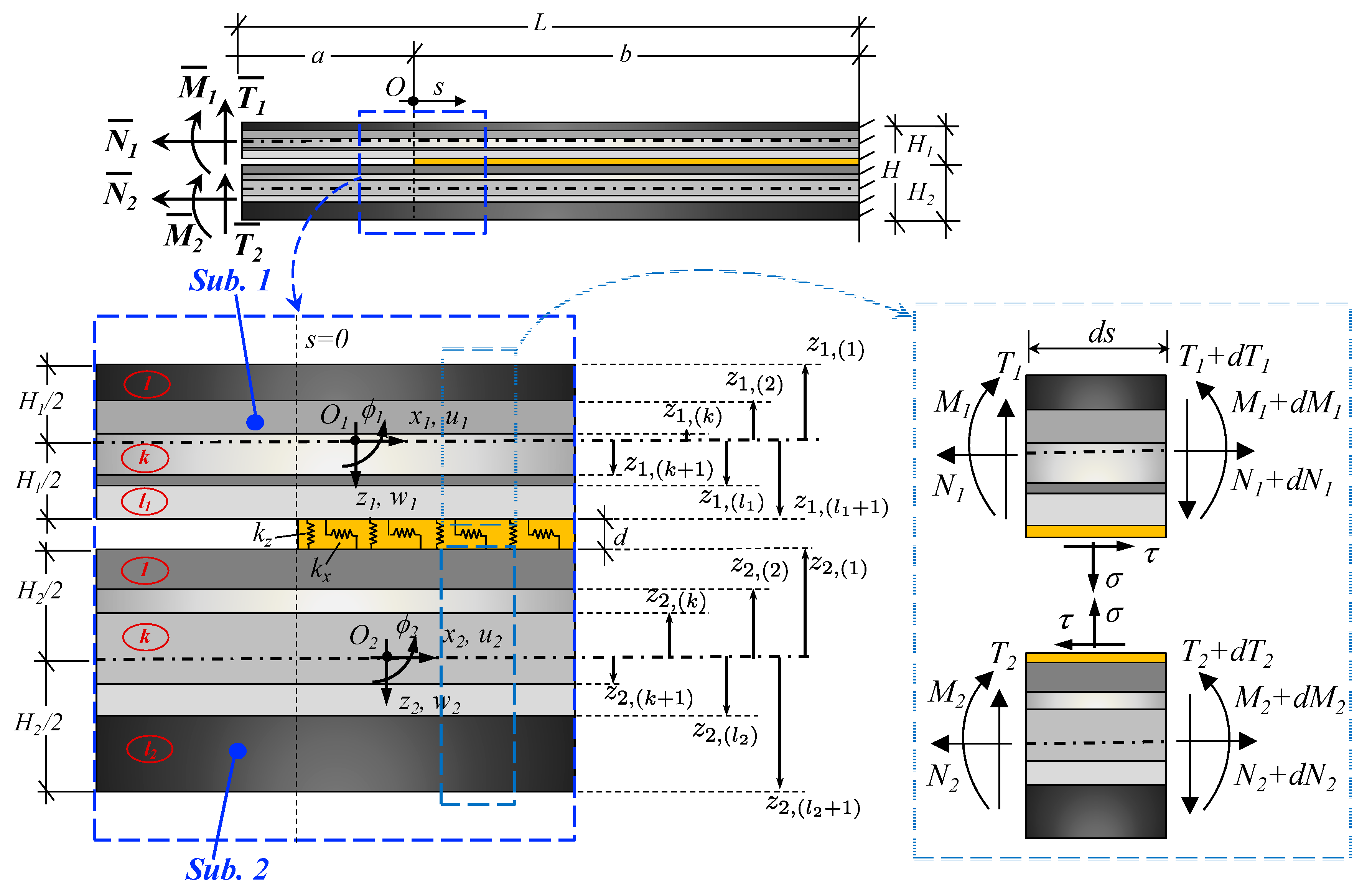
Consider a layered beam, with total length , precrack length , such that corresponds to the uncracked length. The specimen is made of two orthotropic sublaminates, here labelled as 1 and 2, with layers made of different materials and thicknesses, as well as fibre-reinforced laminae with different orientations. General stacking sequences are allowed by the proposed model, including those with bending-extension coupling but neglecting the out-of-plane effects (namely the torsion, the out-of-plane shear, etc.). The sublaminate thicknesses are indicated as and , respectively, whereas the global thickness of the specimen is . The width of the specimen is generally defined as and for sublaminates 1 and 2, respectively, such that . Each arm of the specimen is loaded at the left side with an external normal force , shear force , or bending moment (see Figure 1), in quasi-static conditions, such that the dimensionless loading ratios , and can be suitably varied from −1 to 1 in order to embrace the whole range of mixed-modes between pure-modes I and II.
The two sublaminates are here modelled as Timoshenko beams, partly connected by an elastic-brittle interface (see Figure 1). Each sublaminate is constituted by laminae, with the layer enclosed generally within the and coordinates from the centreline, such that its thickness is . This means that the total thickness for each arm is equal to , as visible in Figure 1.
The coordinate denotes the general distance of cross sections from the crack tip along the longitudinal direction. Thus, stands for the local reference system for each sublaminate centred at its mid-plane. Accordingly, we define the mid-plane displacements , for each sublaminate, along the axial and transverse directions, respectively and we denote the cross-section rotation , positive if counter-clockwise (Figure 1).
Based on classical lamination theory, the sublaminates are here modelled as homogeneous equivalent beams, while introducing the equivalent stiffnesses, to define their extensional stiffness, bending-extension coupling stiffness, bending stiffness and shear stiffness, respectively, as follows:
where stands for the shear correction factor, here assumed equal to 5/6. The equilibrium equations for sublaminates in the unbroken part (i.e.,) read
being, respectively, the axial and shear forces and bending moments within sublaminates. These actions are strictly related to the normal and tangential interface stresses, defined as:
where , are the relative interface displacements in the transverse and axial directions, respectively, whereas are the kinetic quantities at the bottom surface of sublaminate 1 () and are the kinetic quantities at the top surface of sublaminate 2 (). The mechanical formulation proposed hereafter, is based on the Timoshenko’s beam theory, according to which the transverse displacement maintains constant along the thickness (i.e.,) and the axial displacement varies linearly with the thickness coordinate (i.e., ). Hence, the relative separations are
The constitutive laws for each arm can be expressed as
where
By combining Equations (5), (6) and (2) we obtain the following set of differential equations
which is associated to the following boundary conditions (BCs)
These last relations can be expressed in terms of the kinematic quantities and their derivatives, by adopting Equations (5) and (6). Please, note that in Equation (8).
The differential problem (7) is solved, first, in closed form, for homogeneous, isotropic and unidirectional specimens, after a suitable change of variables, as proposed by Bennati et al. [13] for a similar problem. More in detail, the interfacial stresses are selected as primary unknowns for the analytical solution of the problem. The same is then solved numerically in a discretized GDQ setting, which enables a direct solution of Equation (7) in the kinematic unknowns with a reduced computational effort. Once the accuracy and stability of the proposed GDQ approach has been checked, we perform a parametric study of the delamination response in a static, kinematic and energy sense, for isotropic and orthotropic specimens under different mixed-mode conditions.
3. Analytical Solution Strategy
The closed-form solution of the differential problem (7) is not straightforward and it is here found only for the specimen with homogeneous, isotropic and unidirectional sublaminates. In this case, the sublaminate stiffnesses get as follows
where is the longitudinal Young’s modulus, is the shear modulus and is the second moment of inertia for each sublaminate. Thus, the problem is governed by the following differential equations
which can be redefined as function of the interface stresses, by combining Equations (3) and (4). After some mathematical manipulation, we obtain the following differential equation for the normal interface stress
with
and
The general solution of Equation (11) reads
where constants are computed by enforcing the BCs (8), whereas are the roots of the characteristic equation associated to Equation (14). In addition, the tangential stress is determined by solving the following 1st order differential equation
with defined according to Equation (14). By integration of Equation (15), the tangential stress is found to be equal to
where an additional constant must be determined. By substitution of Equations (14) and (16) into Equation (2) and by integration, we determine the explicit expressions for the internal forces, namely
for the axial forces,
for the shear forces and finally
for the bending moments.
With a similar procedure, we can determine the explicit expressions for the kinematic quantities of each arm. More specifically, the substitution of the internal forces (17)–(19) into Equations (5) and (6) and the integration of the final relations with respect to , yields to the expressions below
for the axial displacements,
for the transverse displacements and lastly
for rotations.
It is worth noticing that the static and kinematic relations in Equations (17)–(22) depend on 12 additional constants , with a total number of constants that has to be determined. In addition to the 12 BCs defined by the relations (8), other 7 relations are required to determine all the unknown constants. These remaining relations are determined by substituting Equations (14), (16), (20)–(22) into Equation (3). More specifically, the following relations can be applied to evaluate the first six constants independently, namely
with , for , whereas the following further constants have been introduced
Upon mathematical manipulation, the remaining 13 constants are computed as a function of the first six ones, namely
After defining the analytical expressions for the kinematic quantities, we can determine the energy release rate as in the following
where denote the normal and tangential interface stresses at the crack tip, defined as
Moreover, we can compute explicitly the mode-mixity angle, as shown below
which is here adopted in the crack-growth criterion of the type [18]
in order to control the delamination stage of the specimen.
4. Numerical Strategy: The GDQ Approach
In this section, we show the main fundamentals about the GDQ approach, as here applied to solve numerically the system of Equation (7) in a discrete form. Based on the GDQ approach, the order of a derivative at a coordinate can be computed as a weighted linear sum of the functional values collocation points as follows
where is the total number of collocation points for the discretization of domain along the directions, whereas denotes the weighting coefficients determined with the formulae by Shu and Richards [23,24], for and
In Equation (48), stands for the weighting coefficients for the first-order derivatives defined below
A key aspect of the GDQ approach is dictated by its efficient and accurate application, which is in turn related to the appropriate selection of grip points within the domain. Among different possible choices of grid point distributions, non-uniform discretizations represent an efficient way to ensure more accurate results compared to the uniform option, in agreement with findings by Shu [25] and some comparative evaluations, as found in [26,27]. In this context, a preliminary convergence analysis is performed for varying grid distributions, in terms of the traction vector along the adhesive interface. This is defined by its normal and tangential components , respectively, as follows
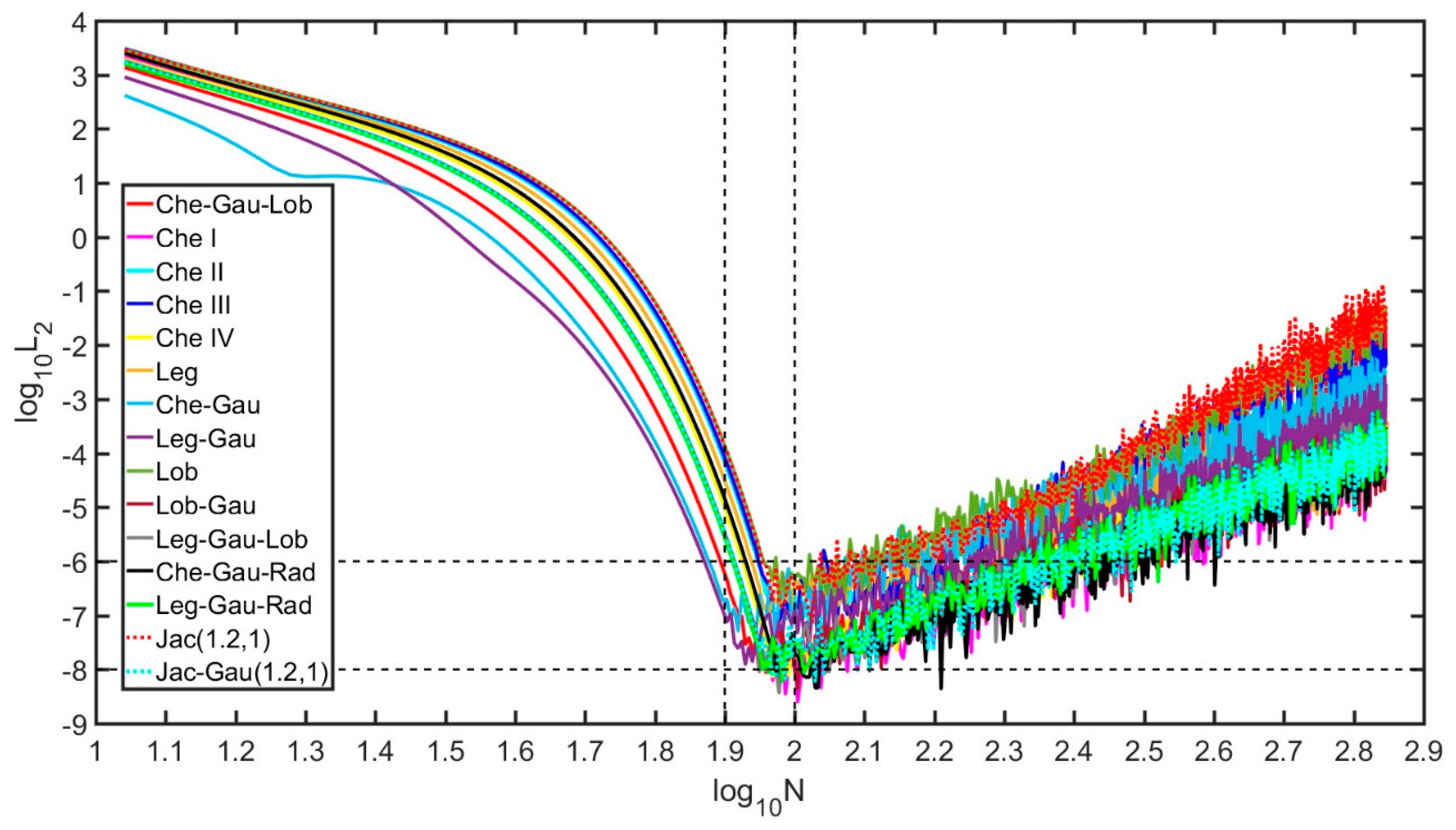
More in detail, the following grid distributions are evaluated comparatively, that is, Che-Gau-Lob, Chebyshev I (Cheb I), Chebyshev II (Cheb II), Chebyshev III (Cheb III), Chebyshev IV (Cheb IV), Legendre (Leg), Chebyshev-Gauss (Cheb-Gau), Legendre-Gauss (Leg-Gau), Lobatto (Lob), Lobatto-Gauss (Lob-Gau), Legendre-Gauss-Lobatto (Leg-Gau-Lob), Chebyshev-Gauss-Radau (Che-Gau-Rad), Legendre-Gauss-Radau (Leg-Gau-Rad), Jacobi (Jac), Jacobi-Gauss (Jac-Gau), see [28] for more details.
Thus, we measure the convergence rate via the norm of the error for the traction vector distribution as
where and refer to the numerical and analytical interface traction, respectively. The analysis starts considering a symmetric specimen of length , precrack length , width , thicknesses , (i.e., a thickness ratio ). The elastic moduli of the sublaminates are , , , , which correspond to a mechanical ratio ). In addition, for the adhesive interface we assume an elastic stiffness and , in the normal and tangential direction, respectively, as in [13,17]. The mixed-mode specimen is loaded on the left side with vertical forces , (which corresponds to a shear loading ratio ), with axial forces , (i.e., an axial loading ratio ) and with bending moments , (i.e., a bending loading ratio ).
As visible in the curves of Figure 2, the rate of convergence is very fast and almost unaffected by the selected discretization. The method seems very stable and limit the error to with a low number of grid points ranging between and . It follows a round-off error phenomenon for higher discretizations, as already observed in the companion work [17]. Based on the results, a Che-Gau-Lob interpolation with a total number of collocation points will be selected, hereafter, for the numerical investigation. Thus, each collocation point along the interface is defined by its coordinate from the crack tip, as in the following
5. Numerical Examples
This section is devoted to many illustrative examples aimed at investigating the mixed-mode structural response for varying loading, geometry and material conditions, either in an independent or a combined form. Comparison with existing formulations from literature helps to highlight the capability of the proposed mixed-mode EBT to capture the fracturing response.
5.1. Loading Effect
A first parametric investigation aims at analysing the mixed-mode response induced by a varying loading condition for a symmetric specimen with length , precrack length , width , thickness . Each sublaminate is made of a 16-ply unidirectional E-glass/epoxy material with elastic moduli and .
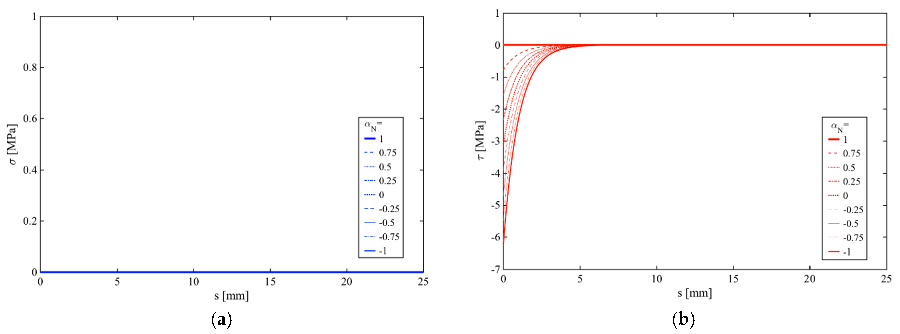
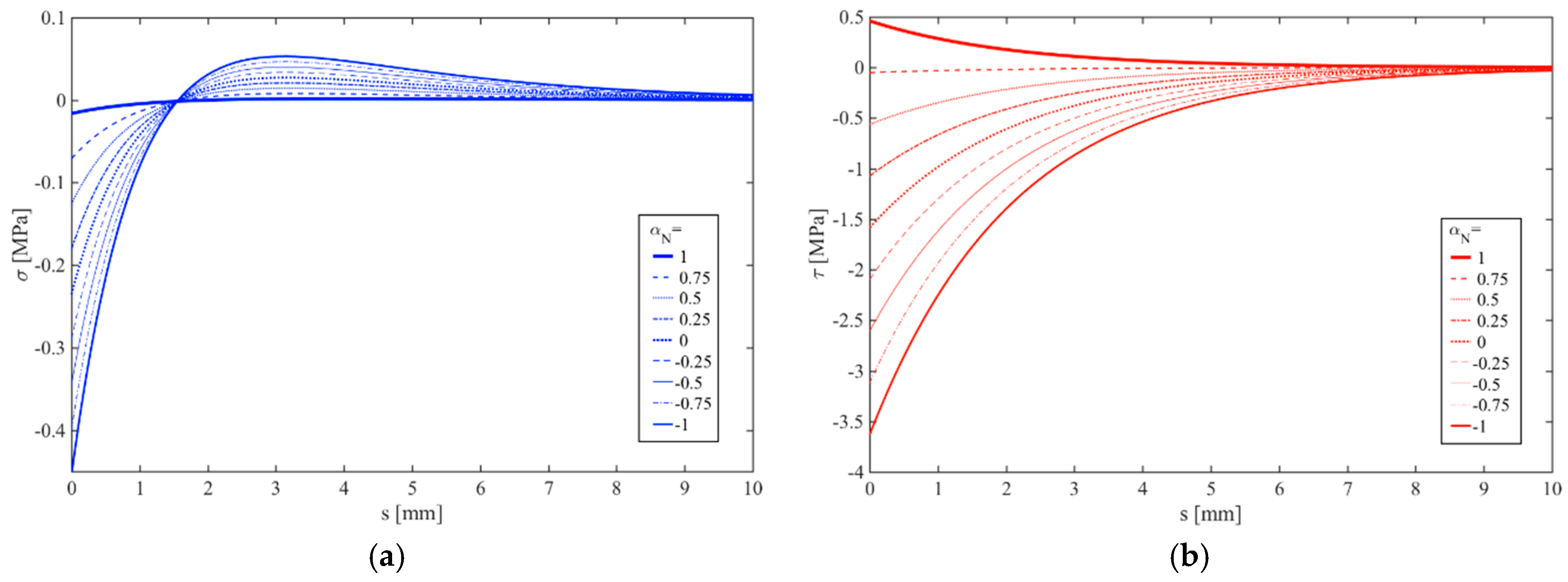
An axial force is applied on the left side of the specimen, while embracing different possible mixed-modes by varying from 1 (pure mode-I) to −1 (pure mode-II). In Figure 3 we plot the structural response in terms of normal and tangential stresses and along the coordinate of the specimen. As visible in Figure 3, the peel stress in the normal direction maintains always null for all mixed-modes, whereas the shear stress reaches the maximum value at the crack tip and decays within a short distance of about 5 mm with a monotonic behaviour. As also expected, the magnitude of the peak values of , reduces gradually moving from pure mode-II to pure mode-I. Only in the last case, vanishes along the whole specimen, which means that the adhesive is completely unloaded.
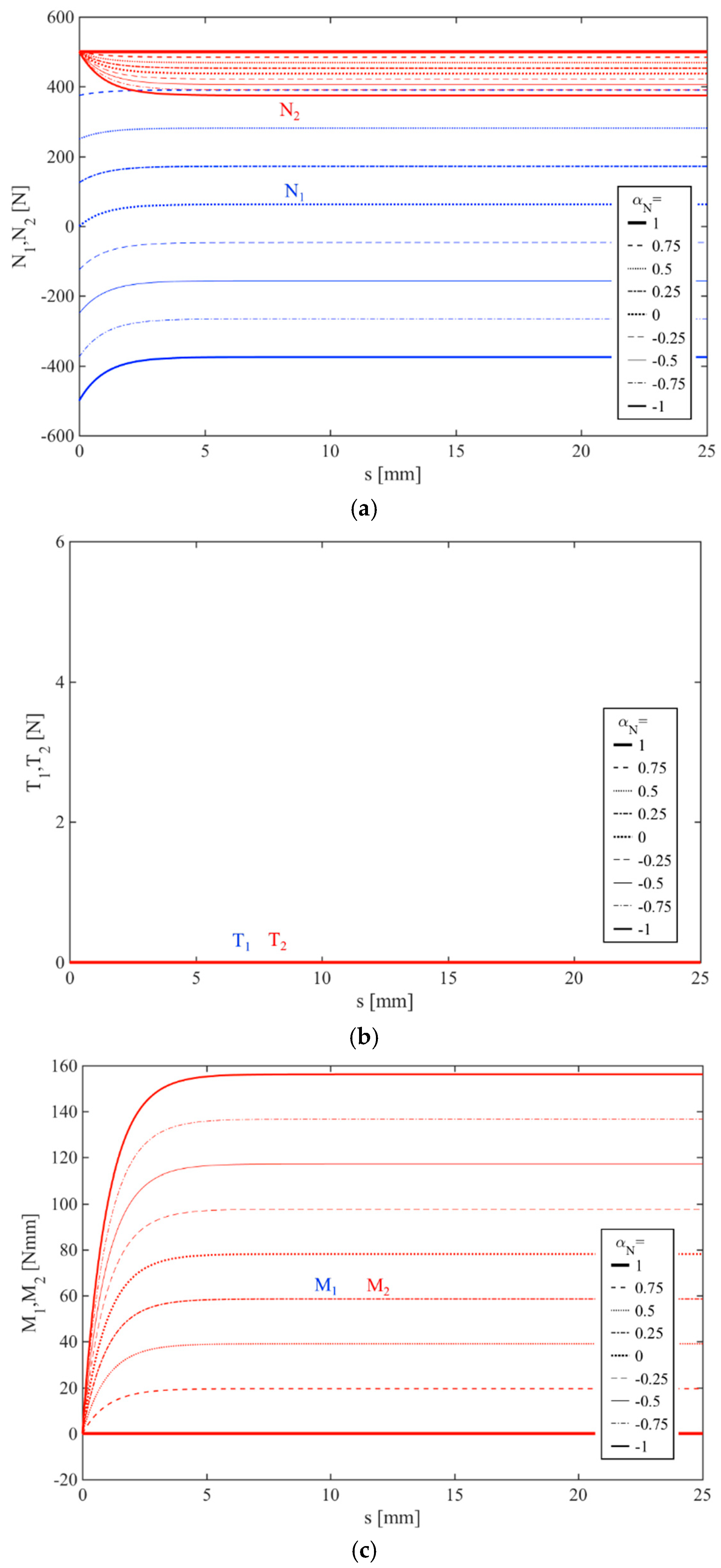
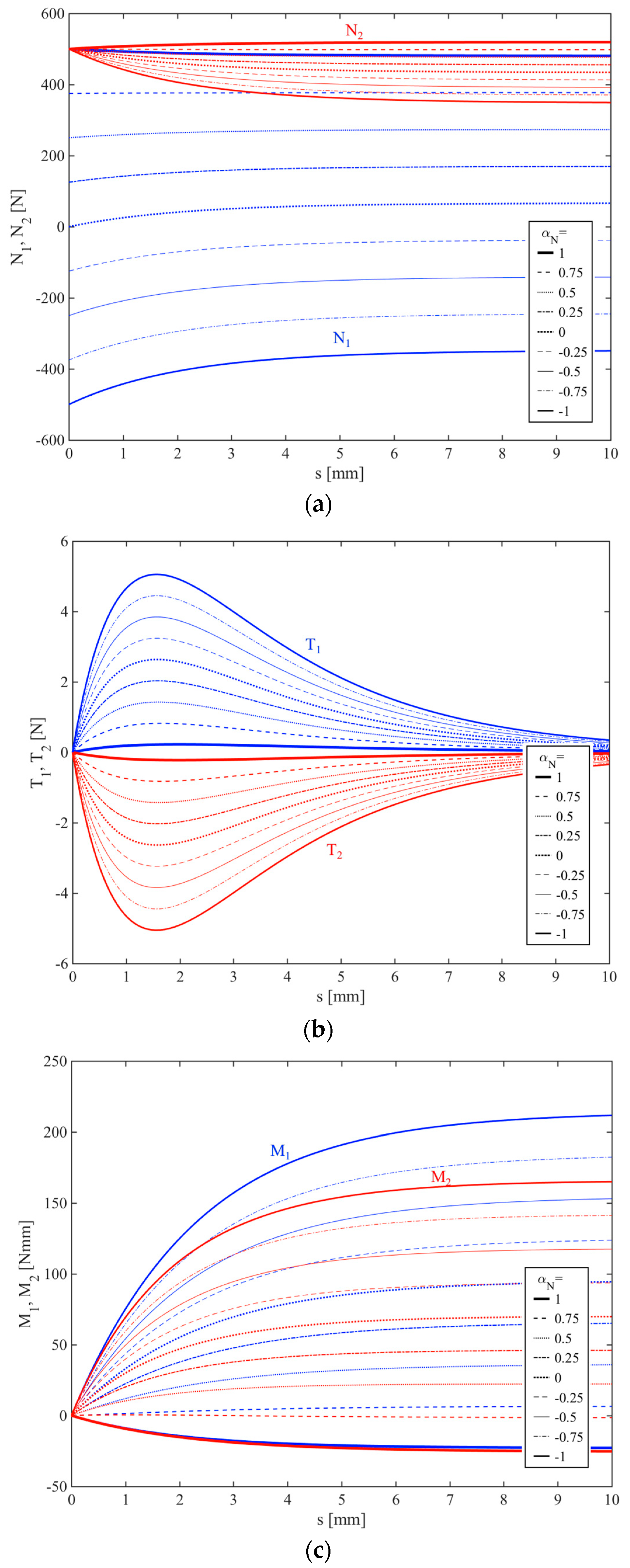
As far as the structural behaviour of the sublaminates is concerned, Figure 4, Figure 5 and Figure 6 present the parametric results in terms of internal forces, kinematic and strain quantities, respectively. More in detail, the axial forces in the two sublaminates are perfectly the same and maintain constant in the whole specimen when (pure mode-I) and assume a symmetric behaviour (i.e., equal in magnitude and opposite in sign) when (pure mode-II). In mixed-mode conditions (i.e., ) feature a monotonic behaviour with a decreasing or increasing trend up to a threshold value within a short distance from the crack tip (see Figure 4a). As also visible in Figure 4b, the internal shear forces are null everywhere within the specimen, while the bending moments are always coincident and different from zero, for both sublaminates, except for pure mode-I for which and do not trigger any bending moment within the specimen (Figure 4c).
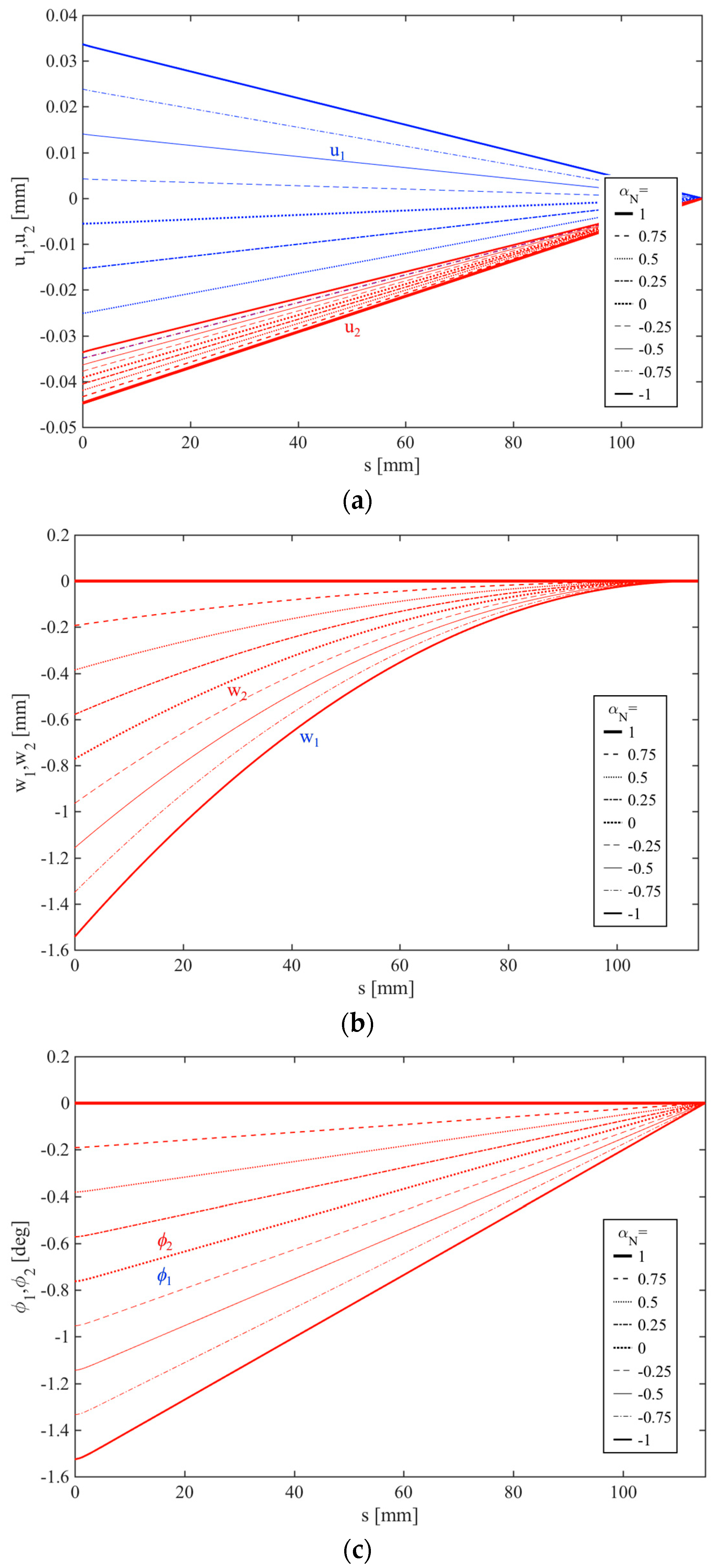
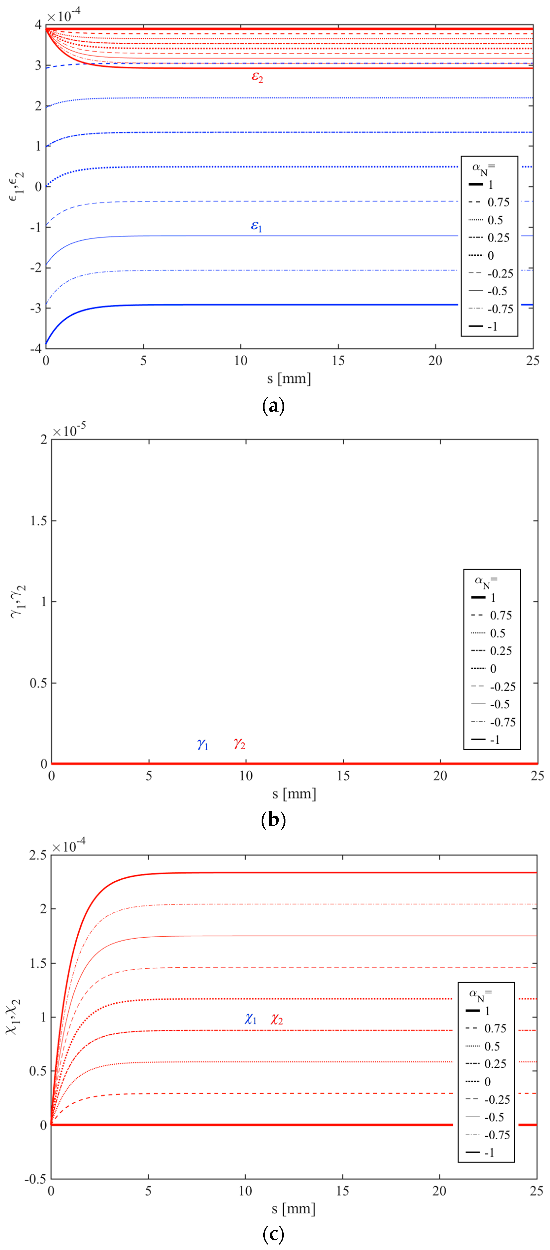
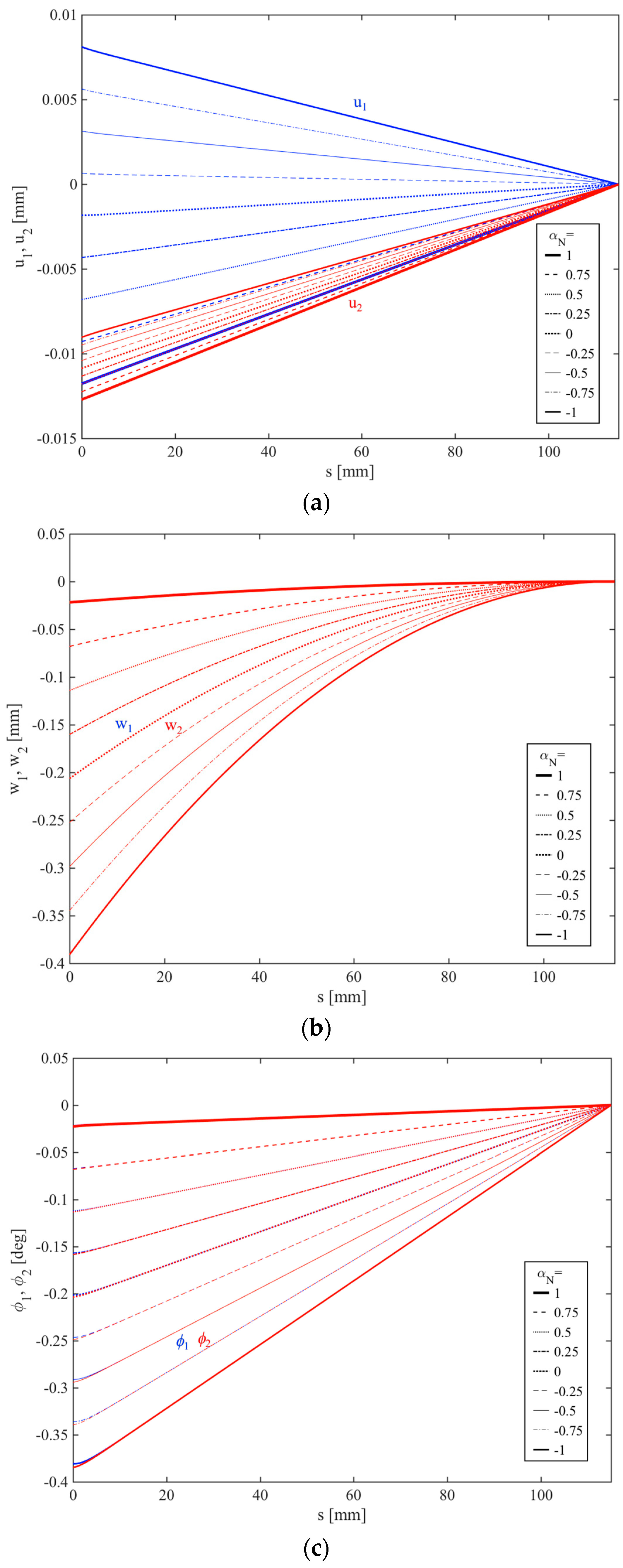
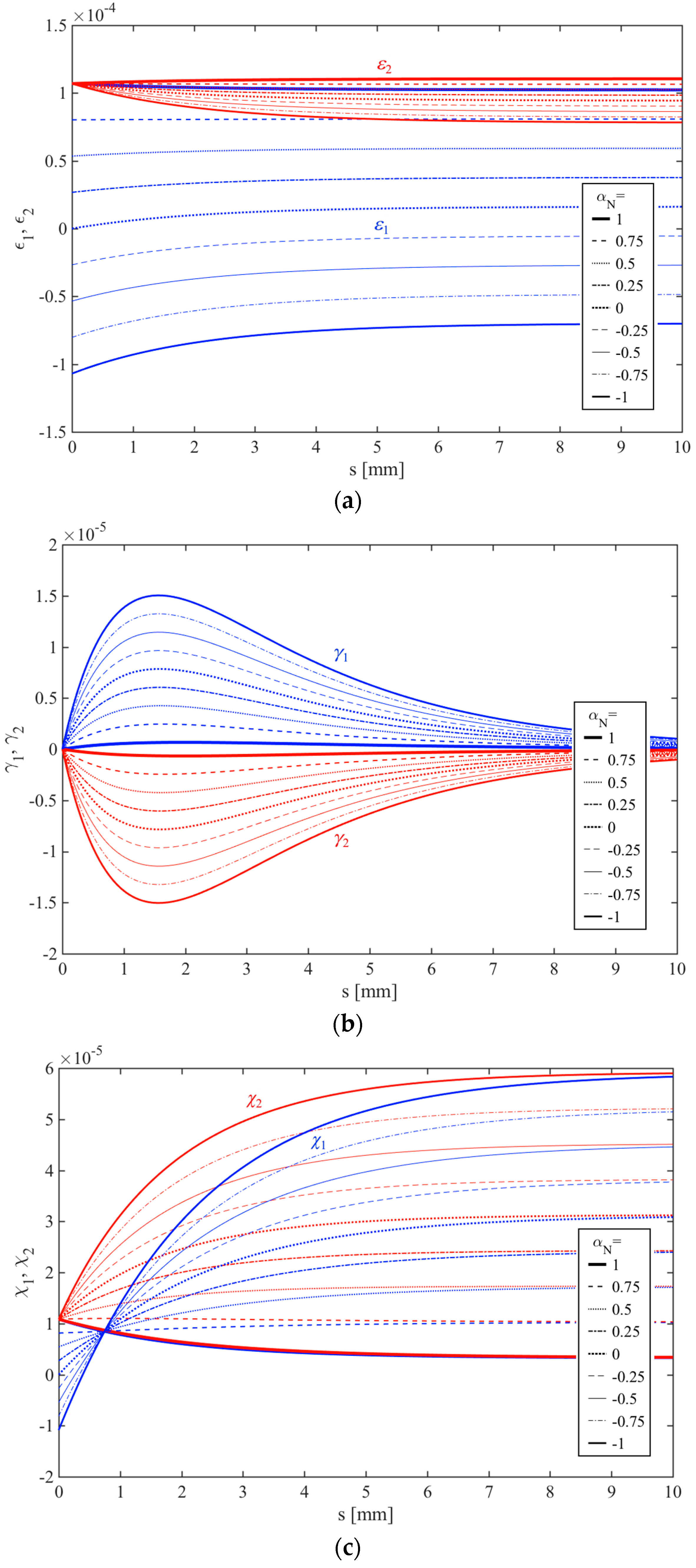
A set of parametric investigations is also repeated in a kinematic sense, as visible in the results plotted in Figure 5. More specifically, Figure 5a represents the axial displacements as computed at the centrelines of sublaminates. These kinematic quantities are always different from zero and vary almost linearly along each sublaminate between a maximum value (for ) and zero at the clamped side of the specimen (for ). In Figure 5b,c, the transverse displacements and rotations are exactly the same in magnitude and sign for all mixed-modes, with the maximum deflection reached at the crack tip of the specimen. By means of the kinematic relations (16), we compute the axial strain , shear strain and curvature of the two sublaminates, whose results are depicted in Figure 6. As expected, for an isotropic specimen under an axial loading, the only deformations involved are the axial and flexural ones.
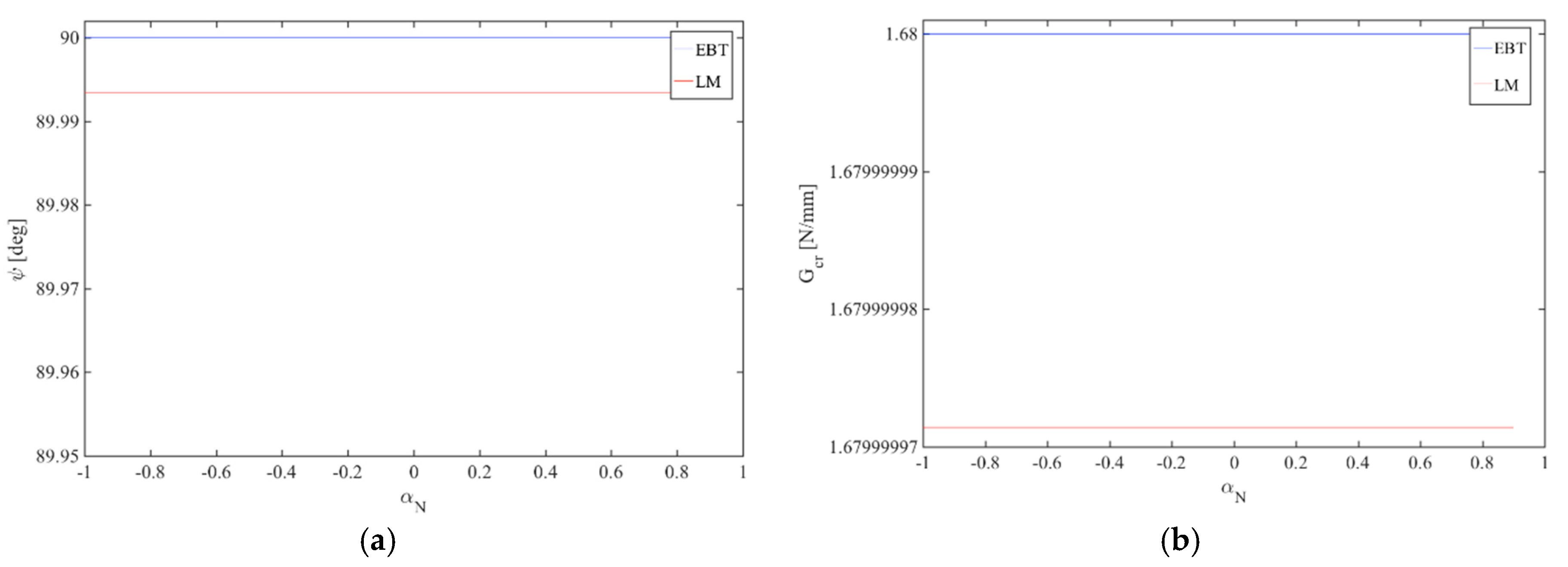
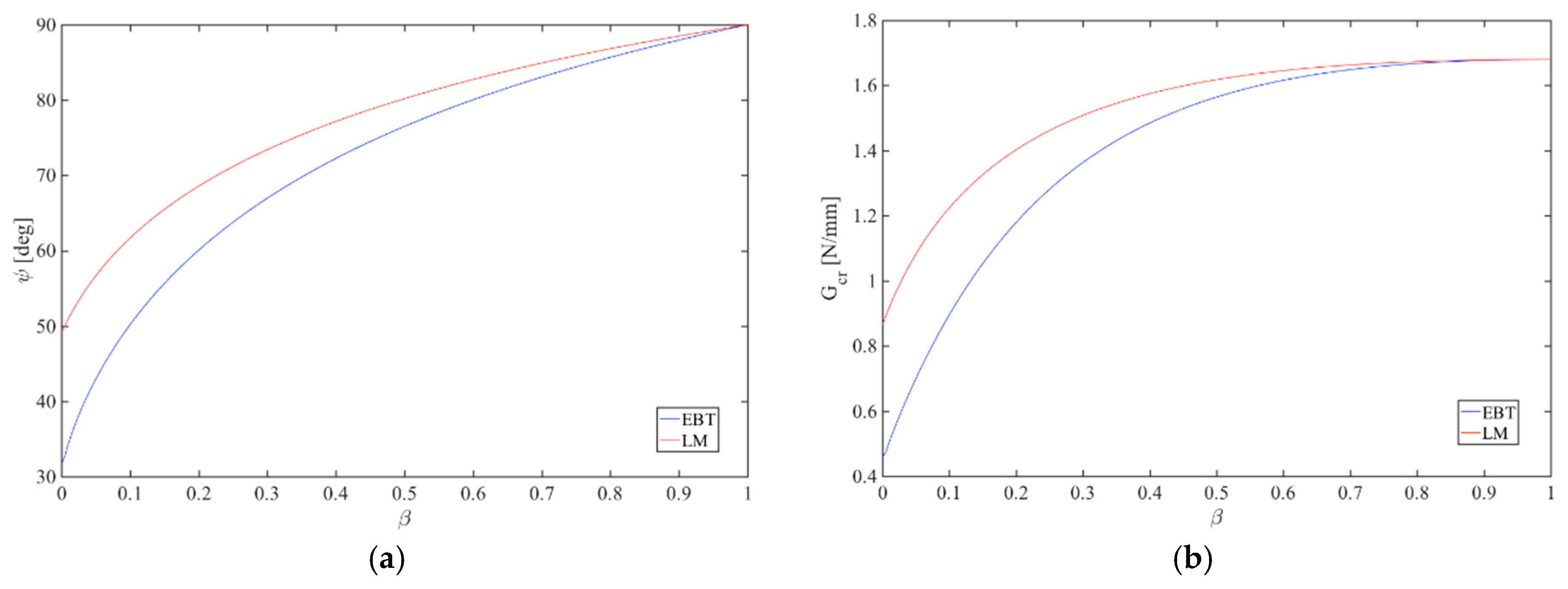
In mixed mode I/II fracture problem, it is well known that the mode-mixity can be characterized by the phase angle of the complex stress-intensity factor. Thus, we compute the mode-mixity angle according to Equation (45) and plot this quantity against the mixed-mode loading ratios (see Figure 7a). A comparative evaluation of the results is also provided with respect to the LM, as proposed in literature by Suo and Hutchinson [18]. According to this last formulation, the shear deformability of sublaminates is not taken into account and does not include any possible dependence of the mode-mixity upon the delamination length . As drawn in Figure 7a, the mode-mixity angle seems to be unaffected by the selected and maintains constant for all mixed-modes (at least for an isotropic specimen, as studied in this first example). The EBT and the LM, in addition, give almost the same results, which proves the validity of the proposed numerical formulation to solve a fracturing problem.
Similar considerations can be also repeated in terms of critical energy which dictates the starting point for the delamination process. Also in this case, the EBT agrees very well with the LM, whose estimations are always lower than predictions based on the EBT. This would have a direct consequence on the global load-displacement response, as will be investigated in a further work.
As second example, we consider a more complex orthotropic specimen, with the following sequence of laminae for each sublaminate: Graphite-Epoxy/Glass-Epoxy/Graphite-Epoxy, of thickness , , (and total thickness ). The Graphite-Epoxy material features a Young’s modulus and shear modulus , whereas the Glass-Epoxy material has a Young’s modulus and shear modulus .
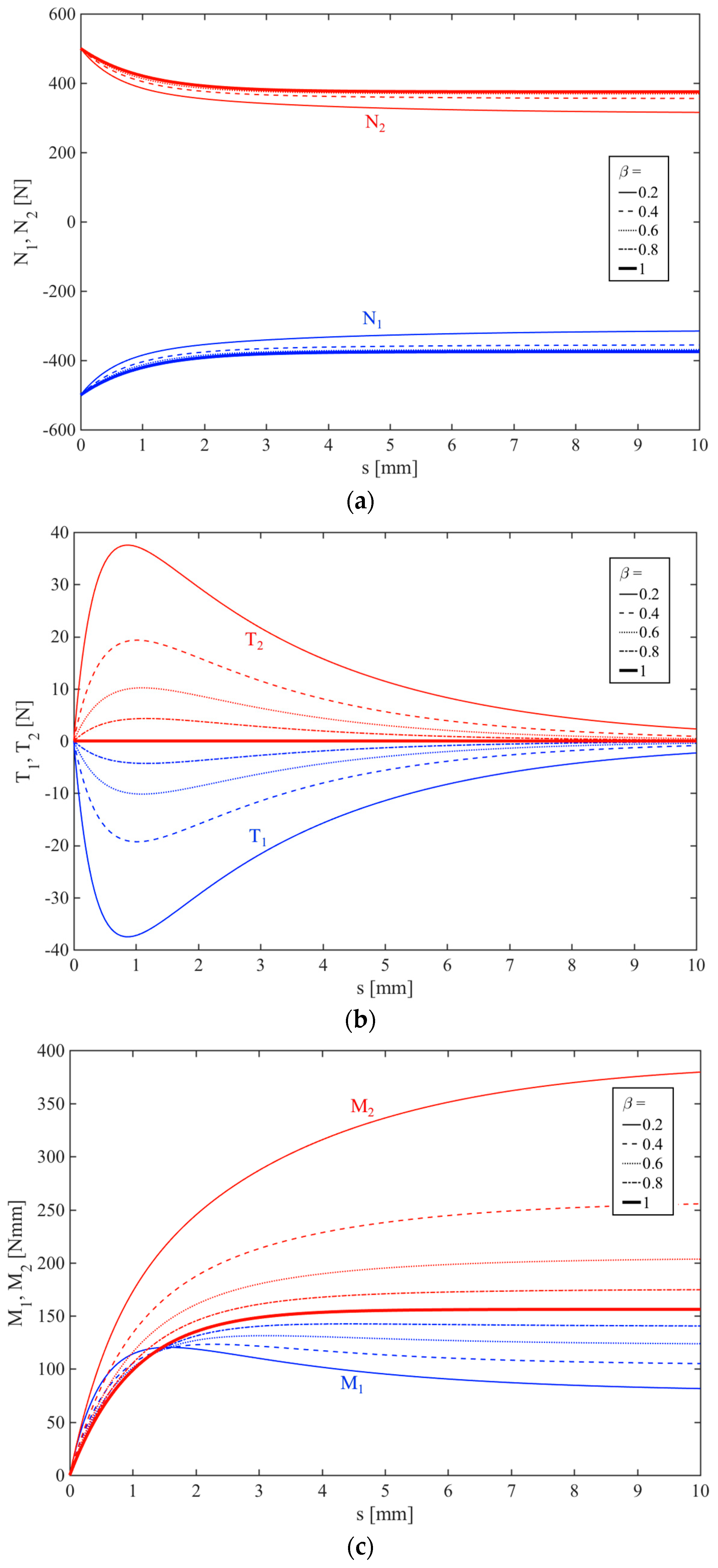
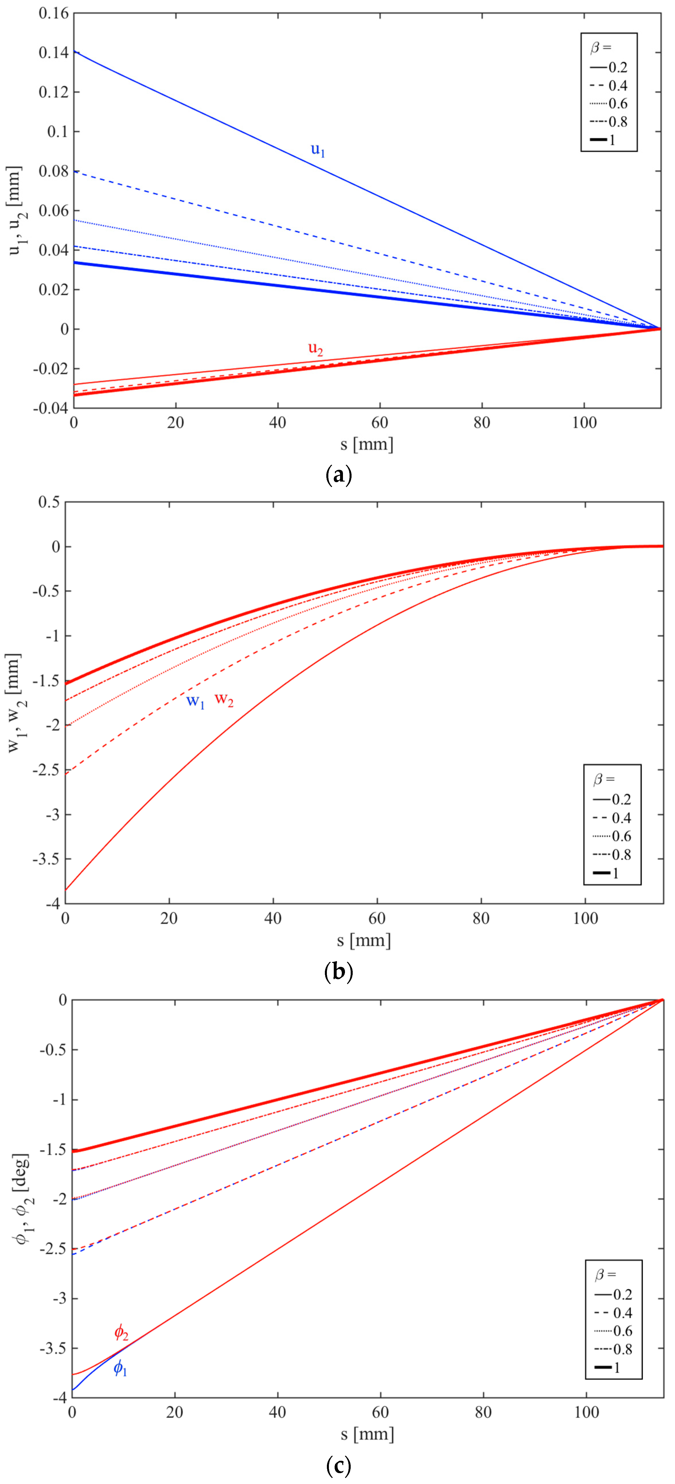
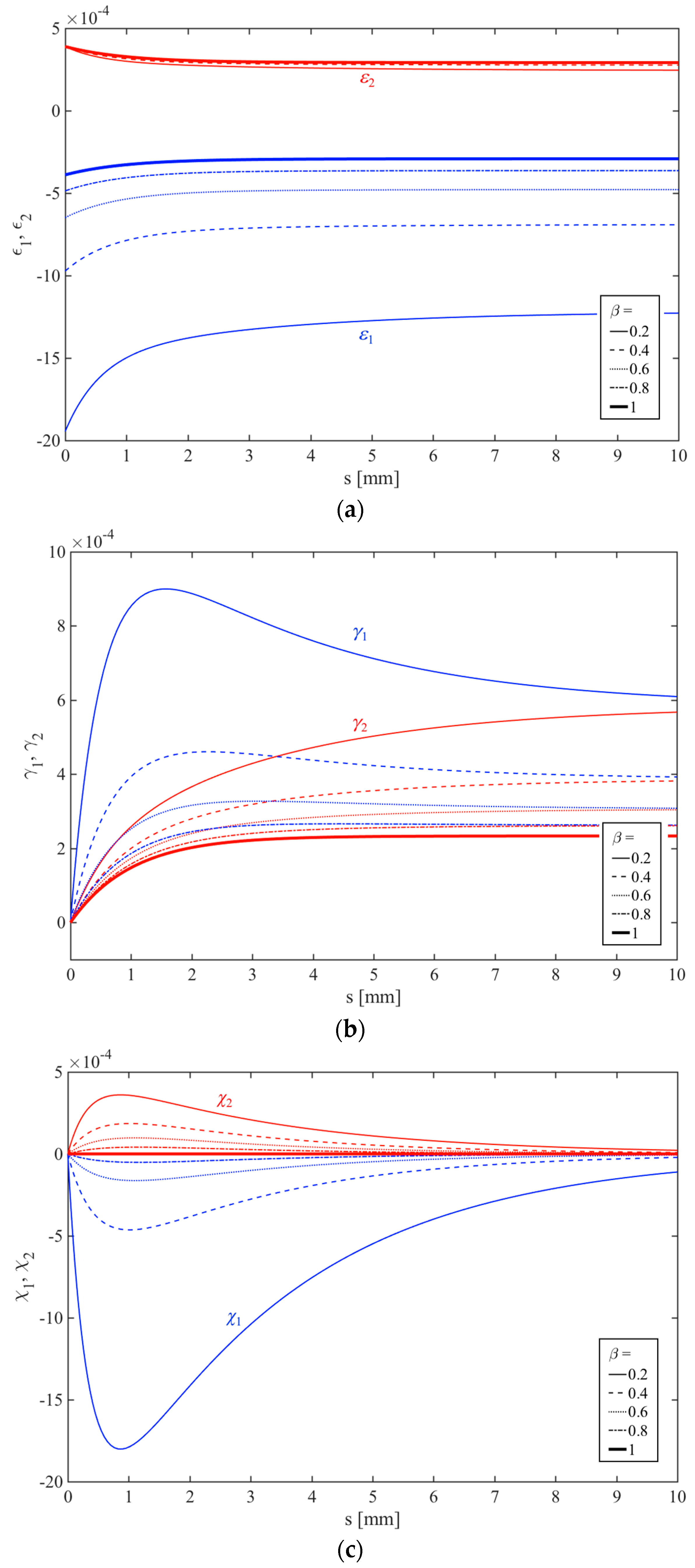
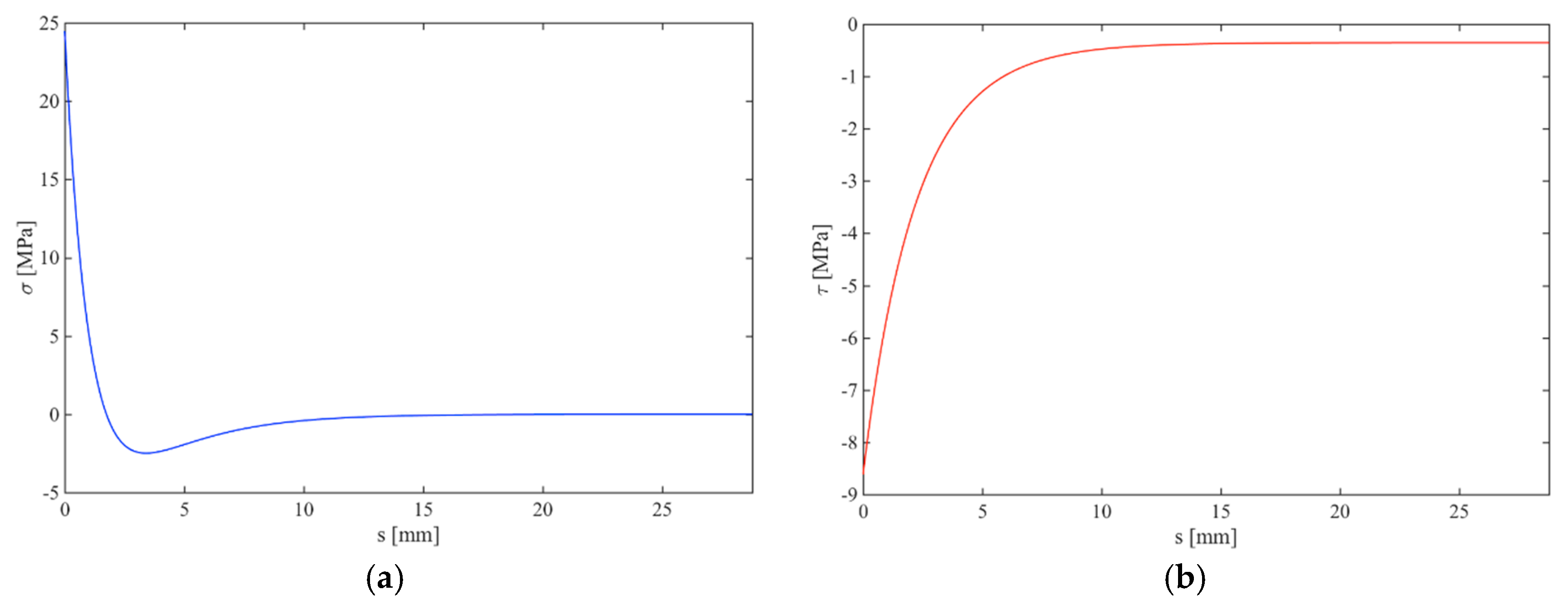
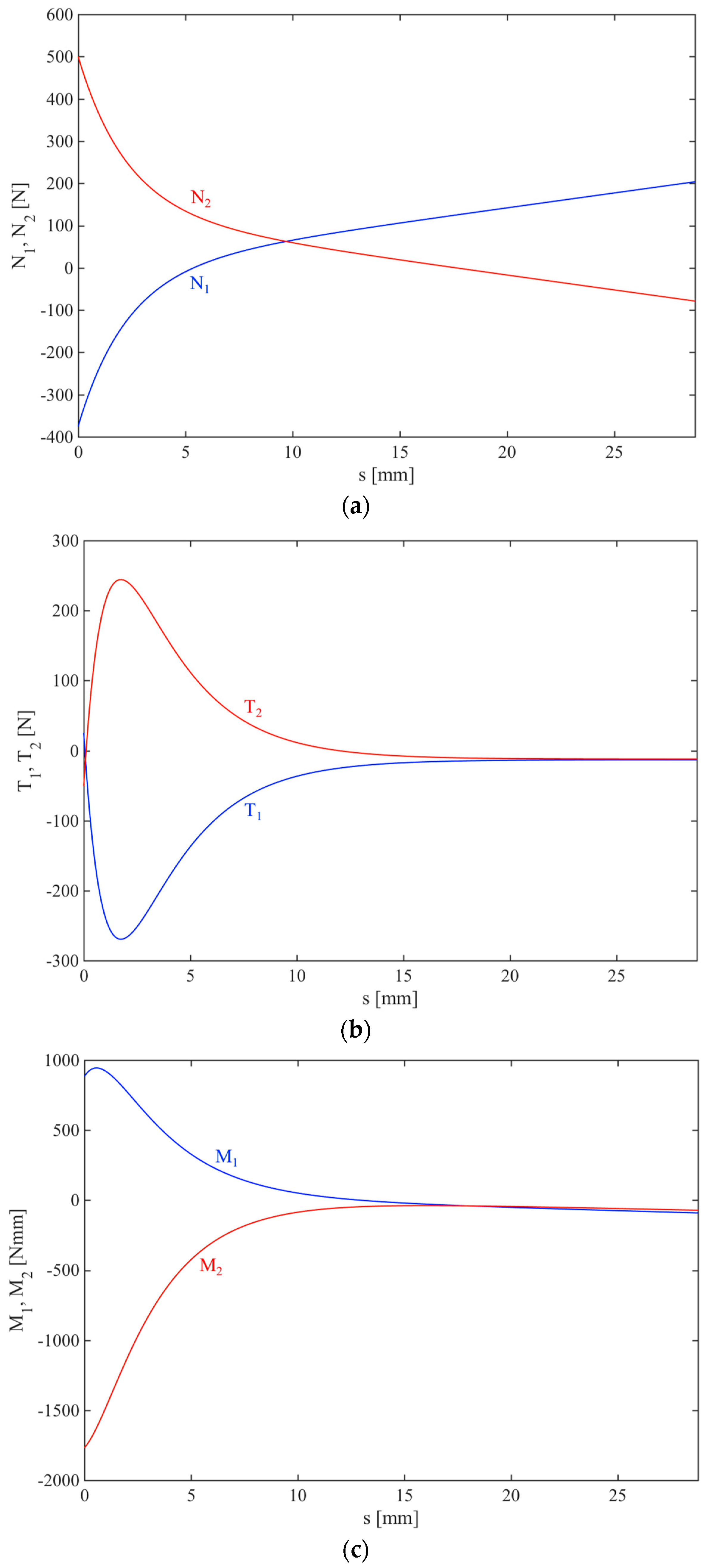
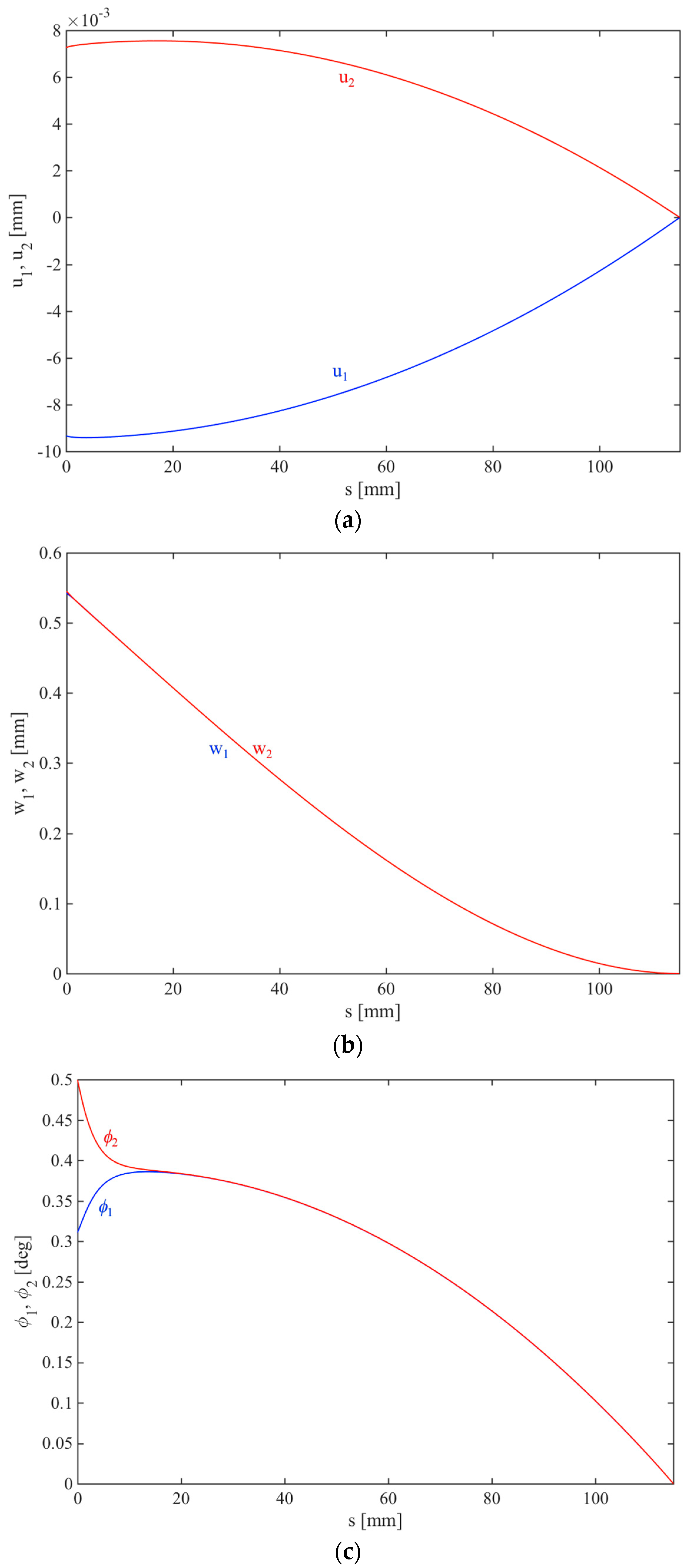
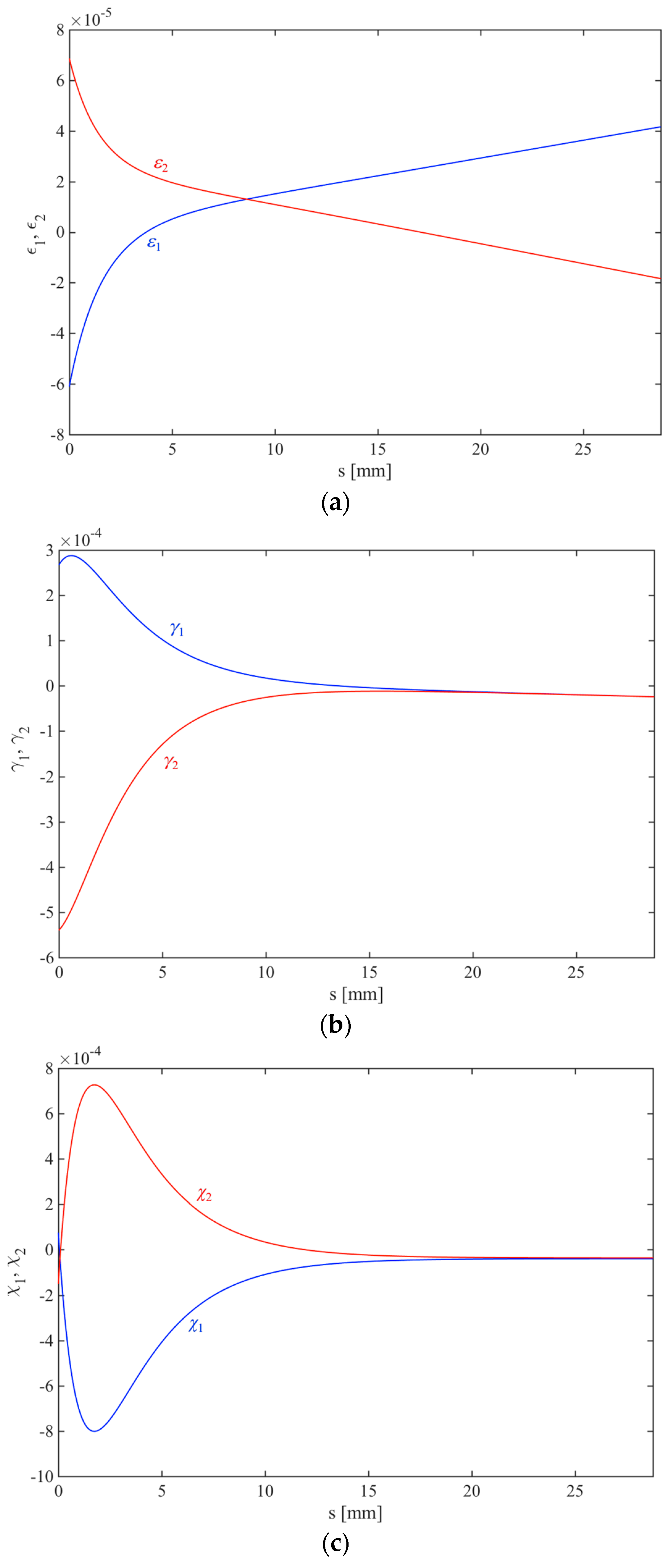
Although a similar problem would be cumbersome to be solved in a closed form, the numerical solution provides an easy and efficient strategy to check for the local response of the specimen, for all mixed-modes. A parametric investigation is then repeated in the static and kinematic sense, as shown in Figure 8, Figure 9, Figure 10 and Figure 11. As visible in these figures, the presence of bending-extension coupling stiffness , for an orthotropic specimen, will always allow to a mixed-mode behaviour both at the interface (see the interface stresses in Figure 8) and within each sublaminate (see the internal forces, displacements and strain in Figure 9, Figure 10 and Figure 11), also for pure-mode loading conditions (namely for ).
5.2. Geometry Effect
Another possible way of studying the mixed-mode delamination is related to the geometry of the specimen, as considered in the foregoing by varying the thickness ratio while assuming a mode-II loading condition with and . The asymmetric DCB has length , precrack length , width and has two sublaminates made of 16-ply unidirectional E-glass/epoxy isotropic material with elastic moduli and . In Figure 12, the numerical solutions in terms of interface stresses and show the high sensitivity to the mixed-mode thickness ratio. More specifically, increased values of the thickness ratio make the oscillating response of and less pronounced. This is due to the increase in stiffness of sublaminate 1 with respect to sublaminate 2. The pure mode-II condition is obtained for a perfectly symmetric specimen, that is, for , which corresponds to the presence of the only tangential stress and a complete absence of the normal component . An increased value of yields to an inversion in sign of (Figure 12a) and to a negligible reduction of (Figure 12b). The consistency of the formulation is also investigated in terms of internal forces and displacements of the sample, as represented in Figure 13 and Figure 14, respectively. As clearly shown in Figure 13a,b, the axial and shear forces and keep always symmetric, independently of the thickness ratio . Bending moments, instead, exhibit always an asymmetric behaviour, except for when a pure mode-II condition is reached (see Figure 13c). A similar consideration can be repeated by analysing the kinematic and strain distributions within sublaminates (see Figure 14 and Figure 15). Moreover, all the displacement components in Figure 14, decay to negligible values within a short distance from the crack tip, in agreement with findings by Bennati et al. [13] and by Dimitri et al. [17]. A further consistency check aims at computing the mixed-mode angle and the critical energy for varying thickness ratios (Figure 16).
The EBT-based numerical results are compared to the theoretical predictions according the LM, with a satisfactory correspondence between them, at least within a certain range of thickness ratios . A non-monotonic variation of both and is observed when applying the EBT approach, instead of an increasing and monotonic trend, as expected by the LM. A perfect correspondence between the two approaches is also reached in pure mode-II condition, when becomes equal to (Figure 16a) and reaches the limit value 1.68 (Figure 16b).
5.3. Mechanical Effect
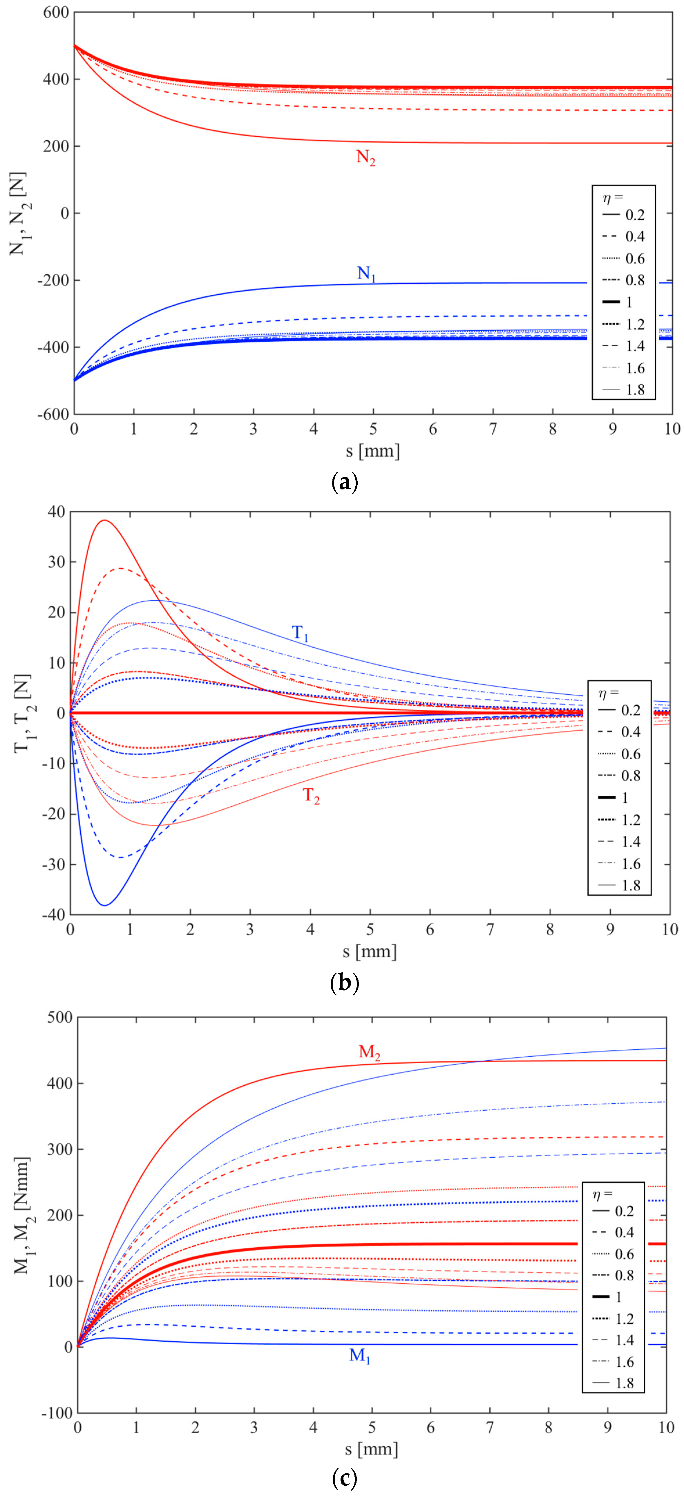
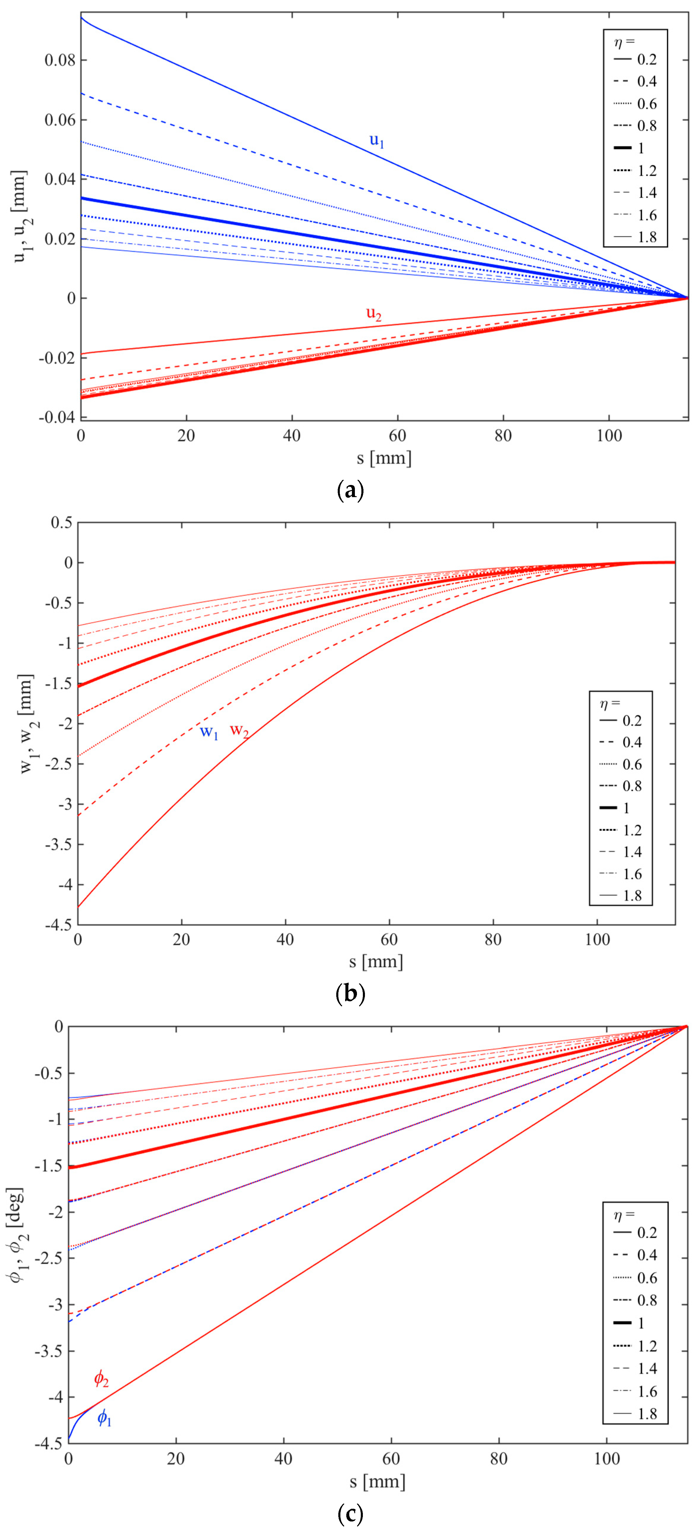
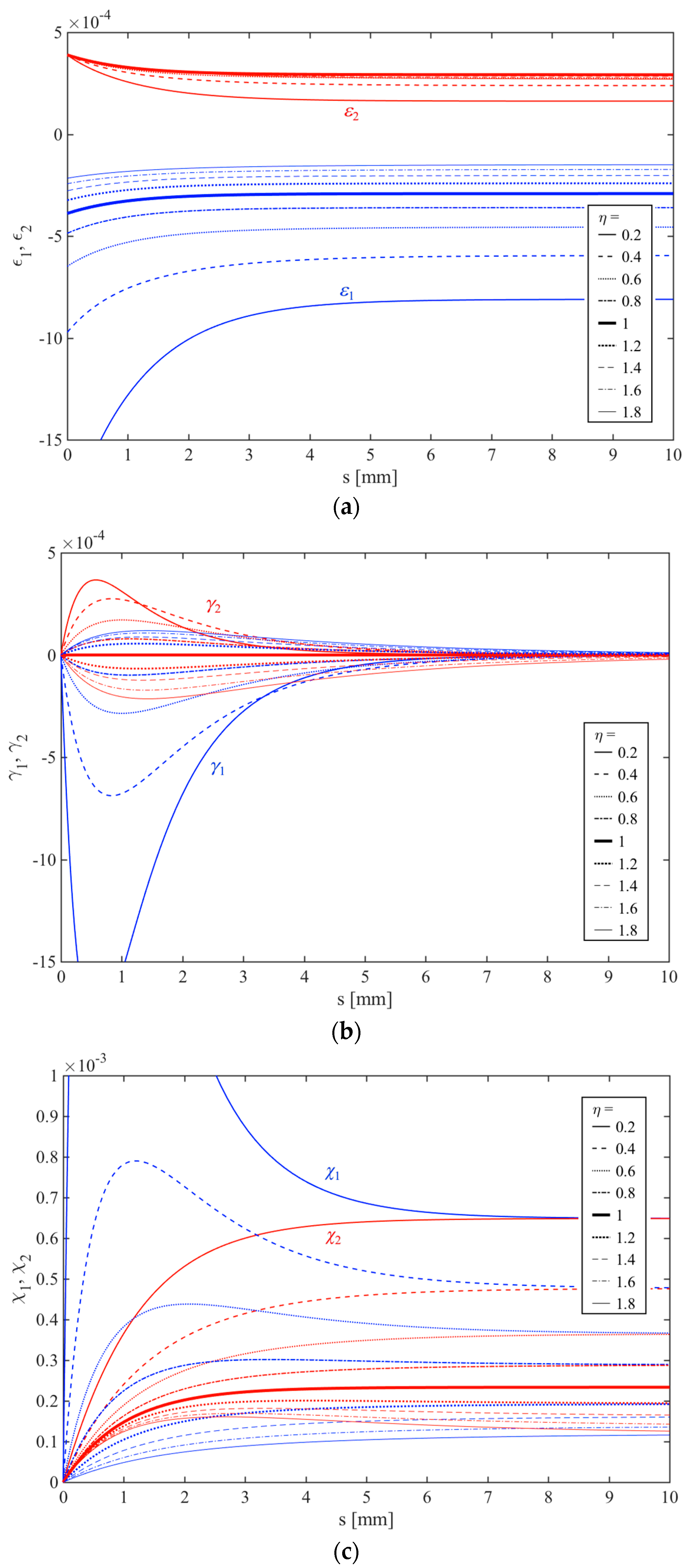
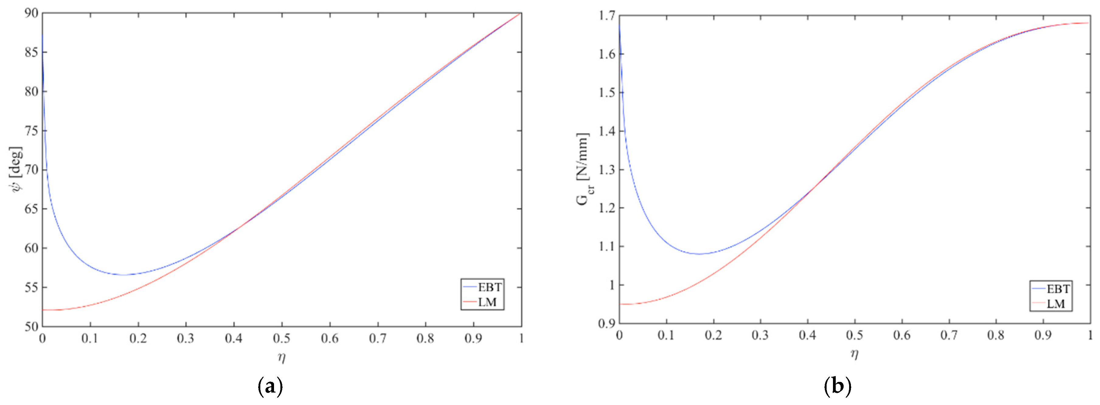
In this section, we analyse the possible effect of the mechanical properties of the specimen on its mixed-mode behaviour, for a fixed pure mode-II loading condition. The elastic properties of sublaminate 1 are related to those ones of sublaminate 2, here set to and . Thus, a dimensionless mechanical parameter is introduced , which is varied from 0.2 to 1, to embrace different possible mixed-modes. A pure mode-II axial loading condition is assumed once again, such that . The local response is plotted in Figure 17 in terms of normal and tangential adhesive stresses and versus the distance from the crack tip. It is worth noticing that an increasing value of corresponds to an increasing stiffness of sublaminate 1, which tends to the one of sublaminate 2 in the limit case given by the condition . Based on the plot in Figure 17, the oscillating behaviour of and features a reduced magnitude for increasing values of . This reverts to a pure condition II when , for which the normal stress becomes zero and only the tangential stress survives along the specimen. Moreover, the outcomes of this parametric study show the variation of the mechanical response of sublaminates for varying mechanical ratios , as clearly represented in Figure 18 in a static sense, as well as in Figure 19 and Figure 20 in a kinematic and strain sense, or, finally in Figure 21 from an energy standpoint (namely and ). More specifically, the plots in Figure 18 show a pronounced sensitivity of the response in terms of shear forces and bending moments and a meaningless variation of the axial forces for varying stiffnesses.
Also, the kinematic and strain response of the specimen is significantly affected by its mechanical properties (see Figure 19 and Figure 20), with a higher deformability of sublaminate 1 compared to sublaminate 2 (Figure 20a–c). Finally, as far as the energy is concerned, the predictions based on the EBT are always more conservative than those ones given by the LM and tend to them when approaching the pure mode condition (see Figure 21a,b).
5.4. Composite Specimen
As last example, we study the mechanical response of the specimen in Section 4, with the same loading conditions but for a more complex composite material. The following sequence of laminae is assumed for each sublaminate: Graphite-Epoxy/Glass-Epoxy/Graphite-Epoxy, of thickness , , and .
Graphite-Epoxy material features a Young’s modulus and shear modulus , whereas the Glass-Epoxy material has a Young’s modulus and shear modulus . This specimen is here selected with the only purpose of demonstrating the great potential and flexibility of the GDQ to solve numerically more complex problems, otherwise cumbersome to be solved in closed form (look at the plots in Figure 22, Figure 23, Figure 24 and Figure 25 for the mixed-mode responses of the interface and sublaminates).
6. Conclusions
In this work, we have proposed the EBT to deal with the delamination behaviour of isotropic and composite specimens under different loading, geometry and mechanical mixed-mode conditions. The specimen is modelled as an assemblage of two sublaminates partly precracked and partly bonded by an elastic interface, here defined through a continuous distribution of elastic-fragile springs in the normal and tangential directions. We check the capability of the GDQ numerical approach to capture the local mechanical response in terms of interface stresses, internal forces, kinematics and deformations within sublaminates, as well as the behaviour in terms of fracture energy and mode-mixity angle. A large parametric investigation is proposed herein to verify the performance and accuracy of the proposed method for delamination problems, even with a reduced computational effort. The numerical EBT approach is compared successfully with some closed-form solutions, where possible and with some predictions available in literature based on a LM. The proposed formulation represents an efficient extension to the one applied in a companion work [17] to moment-loaded DCBs. The same formulation will be expanded in a further work to include elastic-softening cohesive crack interfaces for a deeper understanding of the delamination evolution together with its fracture process zone ahead of the crack tip, as usually occurs within laminated materials and joints.
Author Contributions
The authors R.D. and F.T. contributed equally to the development of the research topic and to the writing of the manuscript.
Acknowledgments
The research topic is one of the subjects of the Centre of Study and Research for the Identification of Materials and Structures (CIMEST)-“M. Capurso” of the University of Bologna (Italy).
Conflicts of Interest
The authors declare no conflict of interest.
References
- Williams, J.G. Fracture Mechanics of Anisotropic Materials; Application of Fracture Mechanics to Composite Materials; Friederich, K., Ed.; Elsevier Science Publishers: Amsterdam, The Netherlands, 1989. [Google Scholar]
- Hashemi, S.; Kinloch, A.J.; Williams, J.G. The analysis of interlaminar fracture in unidirectional fibre-polymer composites. Proc. R. Soc. A 1990, 427, 173–190. [Google Scholar] [CrossRef]
- Reeder, J.R.; Crews, J.H. Redesign of the mixed-mode bending delamination test to reduce nonlinear effects. J. Compos. Technol. Res. 1992, 14, 12–19. [Google Scholar]
- Fernlund, G.; Spelt, J.K. Mixed-mode fracture characterization of adhesive joints. Compos. Sci. Technol. 1994, 50, 441–449. [Google Scholar] [CrossRef]
- Williams, J.G. On the calculation of energy release rates for cracked laminates. Int. J. Fract. 1988, 36, 101–119. [Google Scholar] [CrossRef]
- Suo, Z.; Hutchinson, J.W. Interface crack between two elastic layers. Int. J. Fract. 1990, 43, 1–18. [Google Scholar] [CrossRef]
- Suo, Z. Delamination specimens for orthotropic materials. ASME J. Appl. Mech. 1990, 57, 627–634. [Google Scholar] [CrossRef]
- Li, S.; Wang, J.; Thouless, M.D. The effects of shear on delamination of beam-like geometries. J. Mech. Phys. Solids 2004, 52, 193–214. [Google Scholar] [CrossRef]
- Andrews, M.G.; Massabò, R. The effects of shear and near tip deformations on energy release rate and mode mixity of edge-cracked orthotropic layers. Eng. Fract. Mech. 2007, 74, 2700–2720. [Google Scholar] [CrossRef]
- Bruno, D.; Greco, F. Mixed mode delamination in plates: A refined approach. Int. J. Solids Struct. 2001, 38, 9149–9177. [Google Scholar] [CrossRef]
- Qiao, P.; Wang, J. Novel joint deformation models and their application to delamination fracture analysis. Compos. Sci. Technol. 2005, 65, 1826–1839. [Google Scholar] [CrossRef]
- Alfredsson, K.S.; Högberg, J.L. Energy release rate and mode-mixity of adhesive joint specimens. Int. J. Fract. 2007, 144, 267–283. [Google Scholar] [CrossRef]
- Bennati, S.; Colleluori, M.; Corigliano, D.; Valvo, P.S. An enhanced beam-theory model of the asymmetric double cantilever beam (ADCB) test for composite laminates. Compos. Sci. Techol. 2009, 69, 1735–1745. [Google Scholar] [CrossRef]
- Bennati, S.; Fisicaro, P.; Valvo, P.S. An enhanced beam-theory model of the mixed-mode bending (MMB) test—Part I: Literature review and mechanical model. Meccanica 2013, 48, 443–462. [Google Scholar] [CrossRef]
- Bennati, S.; Fisicaro, P.; Valvo, P.S. An enhanced beam-theory model of the mixed-mode bending (MMB) test—Part II: Applications and results. Meccanica 2013, 48, 465–484. [Google Scholar] [CrossRef]
- Valvo, P.S. On the calculation of energy release rate and mode mixity in delaminated laminated beams. Eng. Fract. Mech. 2016, 165, 114–139. [Google Scholar] [CrossRef]
- Dimitri, R.; Tornabene, F.; Zavarise, G. Analytical and numerical modeling of the mixed-mode delamination process for composite moment-loaded double cantilever beams. Compos. Struct. 2018, 187, 535–553. [Google Scholar] [CrossRef]
- Hutchinson, J.W.; Suo, Z. Mixed mode cracking in layered materials. Adv. Appl. Mech. 1992, 29, 63–191. [Google Scholar]
- Fantuzzi, N.; Dimitri, R.; Tornabene, F. A SFEM-based evaluation of mode-I stress intensity factor in composite structures. Compos. Struct. 2016, 145, 162–185. [Google Scholar] [CrossRef]
- Dimitri, R.; Fantuzzi, N.; Tornabene, F.; Zavarise, G. Innovative numerical methods based on SFEM and IGA for computing stress concentrations in isotropic plates with discontinuities. Int. J. Mech. Sci. 2016, 118, 166–187. [Google Scholar] [CrossRef]
- Dimitri, R.; Trullo, M.; De Lorenzis, L.; Zavarise, G. Coupled cohesive zone models for mixed-mode fracture: A comparative study. Eng. Fract. Mech. 2015, 148, 145–179. [Google Scholar] [CrossRef]
- Dimitri, R.; Cornetti, P.; Mantič, V.; Trullo, M.; De Lorenzis, L. Mode-I debonding of a double cantilever beam: A comparison between cohesive crack modeling and Finite Fracture Mechanics. Int. J. Solids Struct. 2017, 124, 57–72. [Google Scholar] [CrossRef]
- Shu, C.; Richards, B.E. Parallel simulation of incompressible viscous flows by generalized differential quadrature. Comput. Syst. Eng. 1992, 3, 271–281. [Google Scholar] [CrossRef]
- Shu, C.; Richards, B.E. Application of generalized differential quadrature to solve two-dimensional incompressible Navier-Stokes equations. Int. J. Numer. Methods Fluids 1992, 15, 791–798. [Google Scholar] [CrossRef]
- Shu, C. Differential Quadrature and Its Application in Engineering; Springer: Berlin, Germany, 2000. [Google Scholar]
- Quan, J.R.; Chang, C.T. New insights in solving distributed system equations by the quadrature method—I. Anal. Comput. Chem. Eng. 1989, 13, 779–788. [Google Scholar] [CrossRef]
- Bert, C.; Malik, M. Differential quadrature method in computational mechanics. Appl. Mech. Rev. 1996, 49, 1–27. [Google Scholar] [CrossRef]
- Tornabene, F.; Fantuzzi, N.; Ubertini, F.; Viola, E. Strong formulation finite element method based on differential quadrature: A survey. Appl. Mech. Rev. 2015, 67, 1–55. [Google Scholar] [CrossRef]
Figure 1.
Mechanical scheme of the laminated composite specimen.

Figure 2.
error norm of the traction vector at the interface for varying grid distributions.

Figure 3.
Effect of the axial loading on the interface local response: (a) Normal stress; (b) Tangential stress. (Isotropic specimen).
Figure 3.
Effect of the axial loading on the interface local response: (a) Normal stress; (b) Tangential stress. (Isotropic specimen).

Figure 4.
Effect of the axial loading on the static response of the sublaminates: (a) Axial force; (b) Shear force; (c) Bending moment. (Isotropic specimen).
Figure 4.
Effect of the axial loading on the static response of the sublaminates: (a) Axial force; (b) Shear force; (c) Bending moment. (Isotropic specimen).

Figure 5.
Effect of the axial loading on the kinematic response of the sublaminates: (a) Axial displacement; (b) Shear displacement; (c) Cross-sectional rotation. (Isotropic specimen).
Figure 5.
Effect of the axial loading on the kinematic response of the sublaminates: (a) Axial displacement; (b) Shear displacement; (c) Cross-sectional rotation. (Isotropic specimen).

Figure 6.
Effect of the axial loading on the strain field: (a) Axial strain; (b) Shear strain; (c) Curvature. (Isotropic specimen).
Figure 6.
Effect of the axial loading on the strain field: (a) Axial strain; (b) Shear strain; (c) Curvature. (Isotropic specimen).

Figure 7.
Effect of the axial loading ratio on the (a) Mode-mixity angle ; (b) Critical energy . (Isotropic specimen).
Figure 7.
Effect of the axial loading ratio on the (a) Mode-mixity angle ; (b) Critical energy . (Isotropic specimen).

Figure 8.
Effect of the axial loading on the interface local response: (a) Normal stress; (b) Tangential stress. (Orthotropic specimen).
Figure 8.
Effect of the axial loading on the interface local response: (a) Normal stress; (b) Tangential stress. (Orthotropic specimen).

Figure 9.
Effect of the axial loading on the static response of the sublaminates: (a) Axial force; (b) Shear force; (c) Bending moment. (Orthotropic specimen).
Figure 9.
Effect of the axial loading on the static response of the sublaminates: (a) Axial force; (b) Shear force; (c) Bending moment. (Orthotropic specimen).

Figure 10.
Effect of the axial loading on the kinematic response of the sublaminates: (a) Axial displacement; (b) Shear displacement; (c) Cross-sectional rotation. (Orthotropic specimen).
Figure 10.
Effect of the axial loading on the kinematic response of the sublaminates: (a) Axial displacement; (b) Shear displacement; (c) Cross-sectional rotation. (Orthotropic specimen).

Figure 11.
Effect of the axial loading on the strain field: (a) Axial strain; (b) Shear strain; (c) Curvature. (Orthotropic specimen).
Figure 11.
Effect of the axial loading on the strain field: (a) Axial strain; (b) Shear strain; (c) Curvature. (Orthotropic specimen).

Figure 12.
Effect of the thickness ratio on the interface local response: (a) Normal stress; (b) Tangential stress. (Isotropic specimen).
Figure 12.
Effect of the thickness ratio on the interface local response: (a) Normal stress; (b) Tangential stress. (Isotropic specimen).
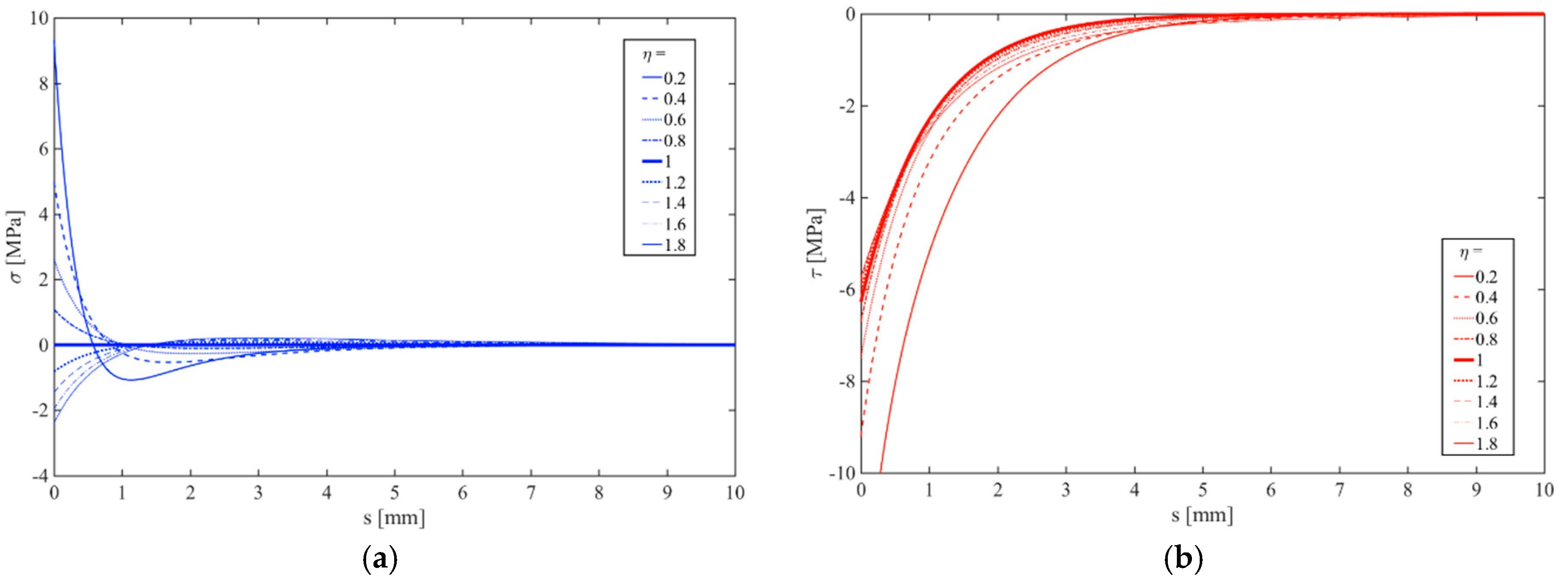
Figure 13.
Effect of the thickness ratio on the static response of the sublaminates: (a) Axial force; (b) Shear force; (c) Bending moment. (Isotropic specimen).
Figure 13.
Effect of the thickness ratio on the static response of the sublaminates: (a) Axial force; (b) Shear force; (c) Bending moment. (Isotropic specimen).

Figure 14.
Effect of the thickness ratio on the kinematic response of the sublaminates: (a) Axial displacement; (b) Shear displacement; (c) Cross-sectional rotation. (Isotropic specimen).
Figure 14.
Effect of the thickness ratio on the kinematic response of the sublaminates: (a) Axial displacement; (b) Shear displacement; (c) Cross-sectional rotation. (Isotropic specimen).

Figure 15.
Effect of the thickness ratio on the strain field: (a) Axial strain; (b) Shear strain; (c) Curvature. (Isotropic specimen).
Figure 15.
Effect of the thickness ratio on the strain field: (a) Axial strain; (b) Shear strain; (c) Curvature. (Isotropic specimen).

Figure 16.
Effect of the thickness ratio on the (a) Mode-mixity angle ; (b) Critical energy . (Isotropic specimen).
Figure 16.
Effect of the thickness ratio on the (a) Mode-mixity angle ; (b) Critical energy . (Isotropic specimen).

Figure 17.
Effect of the mechanical ratio on the interface local response: (a) Normal stress; (b) Tangential stress. (Isotropic specimen).
Figure 17.
Effect of the mechanical ratio on the interface local response: (a) Normal stress; (b) Tangential stress. (Isotropic specimen).

Figure 18.
Effect of the mechanical ratio on the static response of the sublaminates: (a) Axial force; (b) Shear force; (c) Bending moment. (Isotropic specimen).
Figure 18.
Effect of the mechanical ratio on the static response of the sublaminates: (a) Axial force; (b) Shear force; (c) Bending moment. (Isotropic specimen).

Figure 19.
Effect of the mechanical ratio on the kinematic response of the sublaminates: (a) Axial displacement; (b) Shear displacement; (c) Cross-sectional rotation. (Isotropic specimen).
Figure 19.
Effect of the mechanical ratio on the kinematic response of the sublaminates: (a) Axial displacement; (b) Shear displacement; (c) Cross-sectional rotation. (Isotropic specimen).

Figure 20.
Effect of the mechanical ratio on the strain field: (a) Axial strain; (b) Shear strain; (c) Curvature. (Isotropic specimen).
Figure 20.
Effect of the mechanical ratio on the strain field: (a) Axial strain; (b) Shear strain; (c) Curvature. (Isotropic specimen).

Figure 21.
Effect of the mechanical ratio on the (a) Mode-mixity angle ; (b) Critical energy . (Isotropic specimen).
Figure 21.
Effect of the mechanical ratio on the (a) Mode-mixity angle ; (b) Critical energy . (Isotropic specimen).

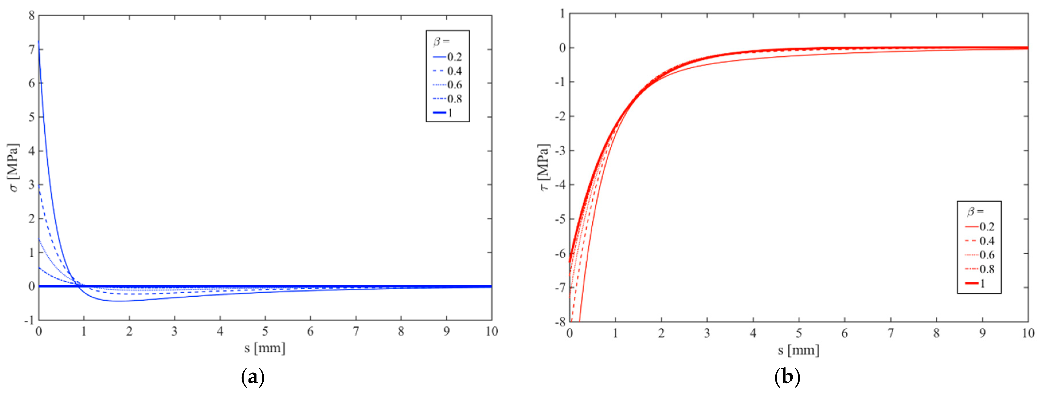
Figure 22.
Composite specimen: (a) Normal stress; (b) Tangential stress.

Figure 23.
Composite specimen: (a) Axial force; (b) Shear force; (c) Bending moment.

Figure 24.
Composite specimen: (a) Axial displacement; (b) Shear displacement; (c) Cross-sectional rotation.
Figure 24.
Composite specimen: (a) Axial displacement; (b) Shear displacement; (c) Cross-sectional rotation.

Figure 25.
Composite specimen: (a) Axial strain; (b) Shear strain; (c) Curvature.

© 2018 by the authors. Licensee MDPI, Basel, Switzerland. This article is an open access article distributed under the terms and conditions of the Creative Commons Attribution (CC BY) license (http://creativecommons.org/licenses/by/4.0/).
Share and Cite
MDPI and ACS Style
Dimitri, R.; Tornabene, F. Numerical Study of the Mixed-Mode Delamination of Composite Specimens. J. Compos. Sci. 2018, 2, 30. https://doi.org/10.3390/jcs2020030
AMA Style
Dimitri R, Tornabene F. Numerical Study of the Mixed-Mode Delamination of Composite Specimens. Journal of Composites Science. 2018; 2(2):30. https://doi.org/10.3390/jcs2020030
Chicago/Turabian StyleDimitri, Rossana, and Francesco Tornabene. 2018. "Numerical Study of the Mixed-Mode Delamination of Composite Specimens" Journal of Composites Science 2, no. 2: 30. https://doi.org/10.3390/jcs2020030