The Cooney Ridge Fire Experiment: An Early Operation to Relate Pre-, Active, and Post-Fire Field and Remotely Sensed Measurements

Abstract

The Cooney Ridge Fire Experiment conducted by fire scientists in 2003 was a burnout operation supported by a fire suppression crew on the active Cooney Ridge wildfire incident. The fire experiment included measurements of pre-fire fuels, active fire behavior, and immediate post-fire effects. Heat flux measurements collected at multiple scales with multiple ground and remote sensors illustrate the spatial and temporal complexity of the fire progression in relation to fuels and fire effects. We demonstrate how calculating cumulative heat release can provide a physically based estimate of fuel consumption that is indicative of fire effects. A map of cumulative heat release complements estimates of ground cover constituents derived from post-fire hyperspectral imagery for mapping immediate post-fire ground cover measures of litter and mineral soil. We also present one-year and 10-year post-fire measurements of overstory, understory, and surface conditions in a longer-term assessment of site recovery. At the time, the Cooney Ridge Fire Experiment exposed several limitations of current state-of-science fire measurement methods, many of which persist in wildfire and prescribed fire studies to this day. This Case Report documents an important milestone in relating multiple spatiotemporal measurements of pre-fire, active fire, and post-fire phenomena both on the ground and remotely.

1. Introduction

Fire behavior (e.g., reaction intensity, spread rate, flame height, and residence time) is related to first-order fire effects such as fuel consumption, stem and soil heating, crown scorch, and smoke production [1,2,3]. Fire behavior also has significant influences on second-order fire effects (e.g., vegetation recovery and succession, erosion, and hydrology) [4], with the effects of a high severity wildfire lasting a decade or longer in forested ecosystems [5].

The complexity of fire behavior makes it difficult to collect spatially explicit measurements that can be related to first- or second-order fire effects [6,7], yet such measurements are critical for understanding the ecological effects of fire. Prior to the late 1990s, much of the data used to describe the behavior and characteristics of wildland fires were derived from post-fire observations, anecdotal evidence, or modeling, rather than from in situ measurements of fire phenomena. When used to develop cause–effect relationships with respect to first- and second-order fire effects, these inferences frequently become circular. That is, the causal agents are described by measuring or observing the effects and are then presented as independent variables with which to draw relationships. Several challenges confront the manager or investigator with respect to in situ measurements of the fire environment. First, it is often difficult to deploy field personnel to locations ahead of a wildland fire that will progress unpredictably. Second, the technology required to characterize the fire environment in such a way as to provide robust thermodynamic data has only recently been developed, and the deployment of these technologies has been largely limited to exploratory research. Finally, such technology that does exist for in situ measurements of the fire environment can only provide point or, at best, spatially disconnected observations. Radiometric measurements of heat transfer currently provide the best means to link fire behavior to fire effects using currently available technologies [8]. Although both convection and radiation are important components of heat transfer [9], radiant heat can be measured remotely, making it more conducive to quantification as a continuous, spatially explicit variable [10].

The ability to create accurate maps of both fire behavior and fire effects could substantively enhance scientists’ and land managers’ ability to associate active fire characteristics with the immediate and long-term response of the post-fire environment. A more complete understanding of these associations could be used either to identify the range of fire behavior characteristics most likely to meet desired prescribed fire objectives or to develop a long-term management plan for a post-wildfire landscape. However, wildland fire is an extremely complex radiant emitter, so any improvements to our understanding of these associations is dependent, first, on a complete characterization of the assumptions and associated error structures inherent to radiometric measurements of fire in wildland fuelbeds on variable terrain and under constantly changing meteorological conditions.

The Cooney Ridge Fire Experiment was designed by fire scientists but coordinated with the incident commander and fire suppression crews managing the Cooney Ridge wildfire incident in 2003. The Cooney Ridge Fire was just one of many explosive wildfire incidents caused by multiple lightning strikes in western Montana during the extremely dry summer of 2003. It was also one of many wildfires simultaneously being actively suppressed. From a fire management perspective, it was conducted as a “burnout” operation to achieve the fire suppression objective of reducing hazardous fuels that could flare up later if left unattended. From a fire science perspective, it was the first “rapid response” research project of its kind. Prior studies [11,12] have already described the values and challenges of conducting rapid response research on the Cooney Ridge Fire and other wildland fires from an organizational and logistical perspective. This research is inherently hazardous, as it is conducted during active wildfire incidents but with appropriate safety measures, and it yields data from before, during, and after fire to better understand fundamental fire processes towards the goal of advancing fire science. The Cooney Ridge Fire Experiment datasets demonstrate how a great variety of multi-scale, spatiotemporal datasets can be collected to tell us something relevant to the fire event and, when considered together, provide synergy in terms of the greater information that can be gained and the lessons learned.

Our objective in this Case Report is to present the primary active and post-fire datasets collected at the Cooney Ridge Fire Experiment that, by virtue of co-location and their complementary spatial and temporal scales, provide the opportunity to relate fire effects to fire radiative energy density (FRED) in a spatially explicit manner. Our primary purpose is to demonstrate that quantitative estimates of FRED obtained by integrating a time series of fire radiative flux density (FRFD) measurements can be combined with post-fire reflectance maps to better characterize the spatial heterogeneity of fire effects, such as percent litter and exposed mineral soil cover [13]. The main reason for choosing to map these variables in this study is that they are important variables for land managers concerned with post-fire rehabilitation treatments to mitigate erosion and promote vegetation recovery [14,15,16].

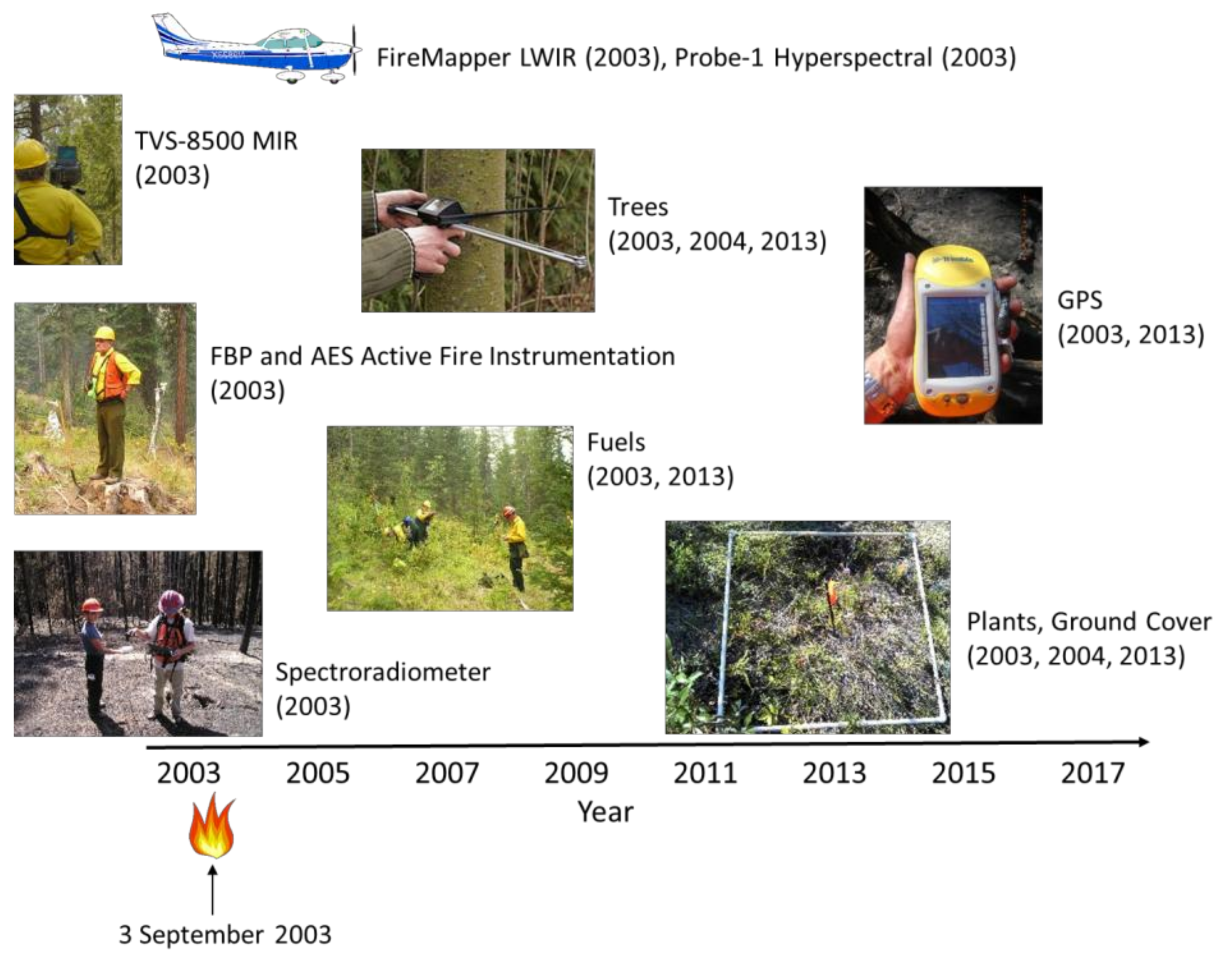
2. Materials and Methods

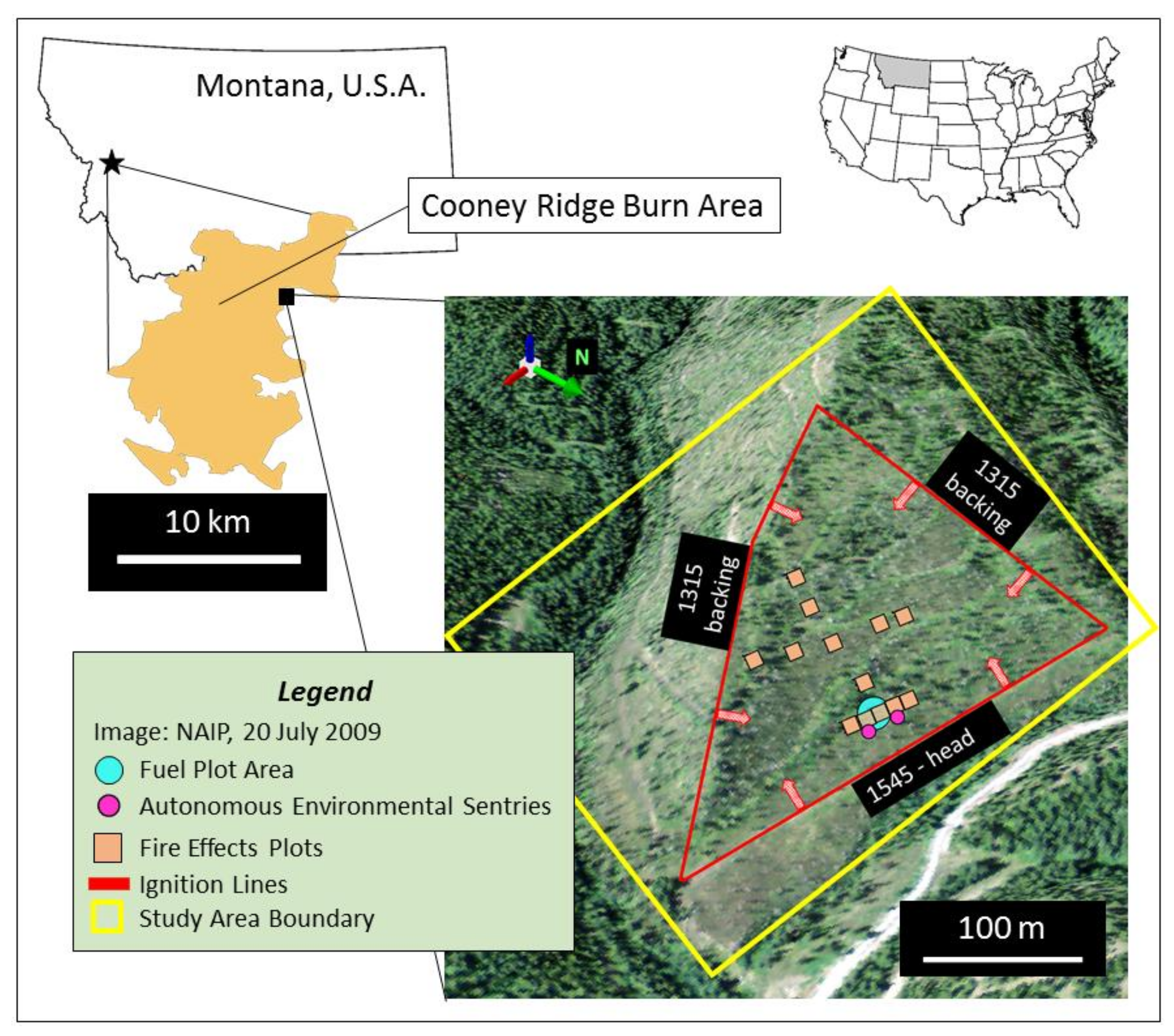
2.1. Study Area

The Cooney Ridge wildfire burned 9600 ha in western Montana from 8 August to 15 October, 2003. A Rapid Response Research team worked with the Incident Command Team to conduct a burnout operation at a safe location within the wildfire perimeter. The chosen site for the experimental burnout was located 26 km southeast of Missoula, Montana (Figure 1) on private industrial forest-owned timberland. The elevation ranged from 1317 to 1446 m at the site, situated on a northeast aspect with a 30% slope (Figure 1). The stand was co-dominated by subalpine fir (Abies lasiocarpa) and Douglas fir (Pseudotsuga menziesii), with a small component of western larch (Larix occidentalis), and understory shrubs comprised primarily ninebark (Physocarpus malvaceus) and snowberry (Symphoricarpos albus).

Figure 1 illustrates the spatial location of in situ ground measurements collected pre-fire (fuel plot), during the fire (fire behavior packages and autonomous environmental sentries), and post-fire (fire effects plots). The full suite of datasets collected both on the ground and remotely in 2003 and years later for monitoring site recovery is illustrated pictorially in Figure 2.

2.2. Fuels and Vegetation

Pre-fire surface fuels and vegetation were characterized on 3 September 2003 (day of the burn) within a single fuel plot situated just upslope of the middle of the northernmost ignition line, which was the last to be lit with drip torches along the bottom slope, after the fire failed to back downslope into the fuel plot from initial ignition lines along the southeast and southwest ridgelines (Figure 1). The plot center was monumented with rebar and a numbered tag, and the location (UTM), slope (%), slope position, and aspect of the plot were recorded. Four plot pictures were taken in the cardinal directions, approximately 3 m from the plot center, facing the plot center.

Fuel loads were measured pre- and immediately post-fire in the fuel plot, such that the consumption of fine and coarse woody debris, litter, and duff could be estimated. Prior to burning, two 22.9 m planar intercept fuel transects [17] were established, beginning at the plot center and radiating out north and east [17]. Each transect was monumented by placing rebar at the end and middle to aid in the post-fire re-installation of the transects. On each transect, we measured the slope (%) and counted the number of 1 h (<0.64 cm) and 10 h (0.64–2.5 cm) fuels along 1.8 m, and of 100 h (2.5–7.6 cm) fuels along 3 m of the transect. We measured the diameter and decay class for 1000 h (>7.6 cm) fuels along 19.8 m of the transect. At two locations on each transect, we recorded the average height of the vegetation in the surface fuel layer (0–1.8 m tall) and total forest floor depth (duff and litter layers combined) using 25 cm spike nails flush with the top of the litter layer. Lastly, we collected ten fuel moisture samples for each of the following components: 1, 10, and 100 h fuel classes, duff, litter, and live fuels. The samples were sealed in plastic bags to prevent moisture loss. Post-fire fuel in the plot was measured the next day after smoldering combustion had ceased. After the fire, the two fuel transects were re-installed and resampled using the same techniques described above. Fine and coarse woody debris and litter consumption were determined by differencing the pre- and post-fire measurements, and forest floor consumption was determined by measuring the length of the spike nail exposed.

Trees were tallied in the fuel plot by tree species, size class, and condition both pre- and post-fire to capture fire-induced tree mortality. Tree diameter at breast height (DBH, 1.37 m above ground), species, and status (live/dead) were recorded for each tree ≥12.7 cm DBH within a 0.04 ha circular macroplot; we also measured total tree height and crown base height. Saplings (<12.7 cm DBH and ≥1.37 m tall) were recorded by species, status, and diameter class on a 0.01 ha circular nested microplot. Seedlings were counted by species, status, and height class on the microplot. Post-fire vegetation was sampled 8 days later on 11 September 2003 to allow time for needle damage due to crown scorch and consumption to become more evident. After re-establishing the plot center, post-fire sampling was conducted using the same techniques as described above. In addition, percent crown volume scorch and scorch height were recorded for each tree in the fuel plot.

Fuel and vegetation data were entered into a FIREMON database [18]. FIREMON was used to calculate fuel loading and summarize vegetation. Fuel samples were weighed within 8 h of collection for wet weight, dried for 8 days at 100 °C, and weighed to determined fuel moisture percentage by size class at the time of the fire.

On 21 September, 2003 thirteen fire effects plots, within which fifteen 1 m × 1 m square subplots were nested in a 3 × 5 grid, were systematically laid out at 20–40 m intervals over the site (Figure 1), following a spatially nested sampling design [19]. The north-central plot was anchored over the fuel plot, and the center fire effects plot was also monumented for longer-term monitoring. Cover fractions of surface materials—soil, ash, char, green vegetation, and non-photosynthetic vegetation (NPV) including litter and other woody debris—were ocularly estimated at the 195 subplots by four trained field technicians. The geolocations of the 13 plot centers were logged with a Trimble ProXR global positioning system (GPS) recording at least 150 positions that were differentially corrected and averaged. All geospatial datasets were projected to UTM Zone 12N (NAD83, GRS 1980).

To monitor site recovery, 6 of the 13 fire effects plots were revisited on 10, 13, or 14 July 2004, and revisited again on 13 August 2013. The site was last revisited on 7 November 2016 to complete a photopoint time series of the fuel plot beginning just prior to the fire experiment on 3 September 2003.

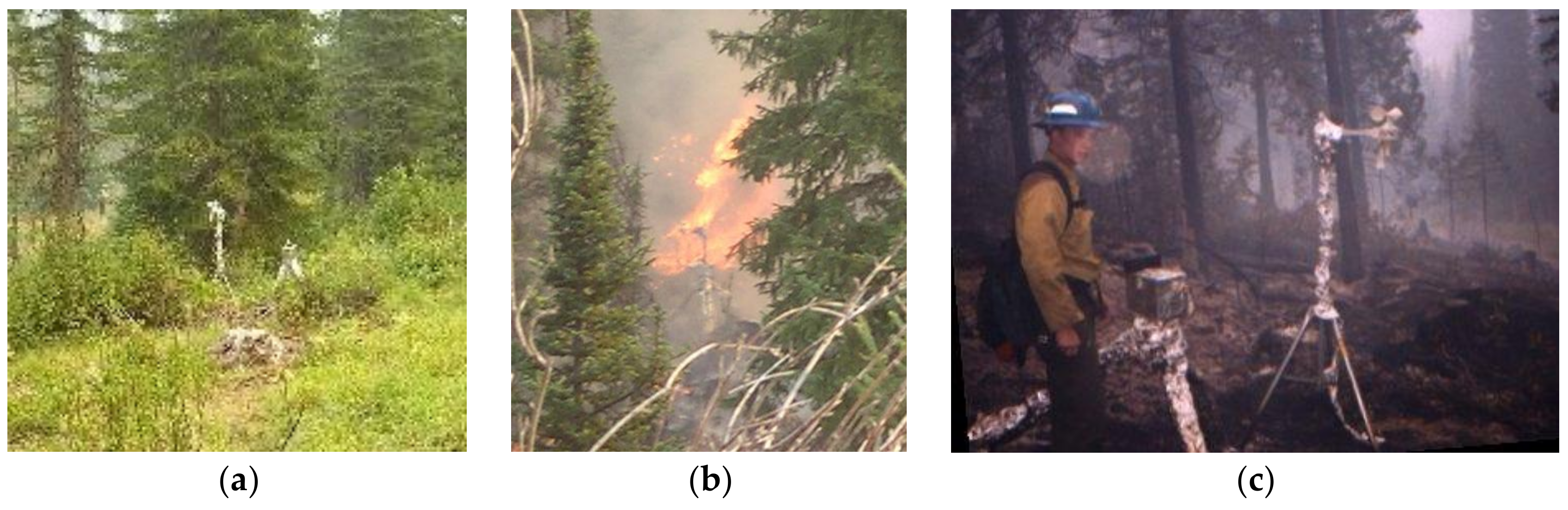
2.3. In Situ Heat Flux and Weather

Fire videography, heat flux, and surface weather data were collected from ground-based sensors installed immediately adjacent to the 0.04 ha fuel plot (Figure 1). Convective and radiative heat flux were measured in situ with thermocouples and side-viewing radiometers mounted in Fire Behavior Packages (FBP) deployed just prior to the burnout experiment. The FBP system, consisting of temperature, air flow, and energy sensors for quantifying energy and mass transport in wildland fires, was used to measure fire spread and intensity [20]. The system contains a programmable datalogger, a Medtherm Dual Heat Flux sensor (Model 64-20T) of the Schmidt-Boelter style that provides incident total and radiant energy flux, a type K fine wire thermocouple (nominally 0.025 mm diameter wire), a custom-designed narrow angle radiometer (NAR) [21], and two pressure-based flow sensors, one oriented to sense horizontal flow and one to sense vertical flow [22]. The sensors were calibrated prior to deployment according to customized procedures [20]. The fine wire thermocouple has a response time of approximately 0.01 s (Omega Engineering) and was used to sense flame presence and residence time. Convective heat flux at the sensor face was calculated by taking the difference between the total and radiant sensors after correcting for transmission through the radiometer window [3].

Also, just prior to the experimental burnout, two Autonomous Environmental Sentries (AES) were deployed on either side of the fuel plot next to the two FBP (Figure 1). The two AES consisted of a custom-designed data logger, broad-band radiometer (0.5–12.50 μm), conventional cup anemometer, wind vane, and relative humidity/temperature sensors. Ambient air temperature and relative humidity were recorded at 1.85 m height above ground, as were wind speed and wind direction. Radiant temperature and radiant heat flux were recorded by the radiometer at 30 s intervals looking downward towards the ground at an angle of 45°, which translates to an area of ~2 m radius. Brightness temperature was calibrated in the laboratory using an equivalent blackbody reference to allow the estimation of the near-surface fire radiative flux density (FRFD). Integrating FRFD over time gives the fire radiative energy density (FRED) which, through laboratory and field experiments, has been shown to be related to total fuel consumption mediated by the radiative fraction, fuel moisture content, fuel distribution, and other combustion parameters [23].

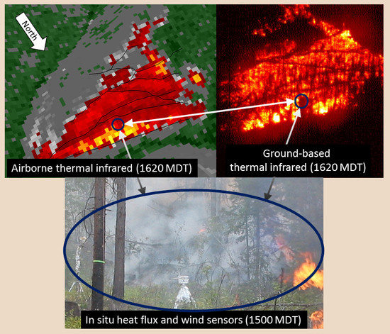
2.4. Thermal Infrared Imagery

Ground-based. A sequence of low-oblique, middle infrared (MIR) images was collected on 3 September 2003 between 15:50 and 17:18 local Mountain Daylight Time (MDT) from a ground-based thermal imaging system (CMC Electronics Cincinnati model TVS-8500) installed on an opposing hillside located 785 m northeast and 176 m above the study site (Figure 1). From this vantage point, the instantaneous field of view (IFOV) of the TVS-8500 provided a nominal ground resolution of 0.8 m. The TVS-8500 has a “twin-peaks” spectral response function, responding to MIR wavelengths between 3.4 μm and 5.1 μm with a CO₂ emission filter between 4.1 μm and 4.5 μm (

Table 1. Instrument specifications for the ground-based Cincinnati TVS-8500 and airborne FireMapper^TM used to collect thermal images of the Cooney Ridge Fire Experiment.

Instrument	Cincinnati TVS-8500	FireMapperTM
Manufacturer	CMC Electronics	Space Instruments
Spectral Bands	3.4–4.1 μm 4.5–5.1 μm	8.1–9.0 μm 11.4–12.4 μm
Image Dimensions	236 × 256 pixels	327 × 205 pixels
Raw Image Resolution	0.8 m	4.5 m
Uncompressed Image Size	121 KB	134 KB
Image Encoding	14 bit	16 bit
Instantaneous Field of View	1 milliradian	1.85 milliradians
Field of View	14.6°	35° (crosstrack)
Sensor Position	785 m horizontal distance 176 m vertical distance	3500 meters AGL

). With the exception of two gaps in acquisition (13 and 5 min), MIR images collected at 2 frames per minute were coregistered and georegistered [24]. Although the 0.04 ha fuel plot subtended 563 pixels in the field of view of the TVS-8500, nearly half of the plot (203 pixels) was obscured by two tree crowns in the foreground.

Active fire pixels (i.e., thermal pixels likely containing flaming and/or smoldering combustion processes) were identified in the low-oblique MIR imagery using a dynamic detection threshold:

$$T\ge {\overline{T}}_r+4{\delta }_{T_r}$$

(1)

where T is the brightness temperature of an individual pixel, and ${\overline{T}}_r$ and ${\delta }_{T_r}$ are the mean and mean absolute deviation of brightness temperatures within a region, r, containing 848 pixels located adjacent to the fuel plot that did not burn. In most applications, the use of a relative detection threshold is designed to account for spatial variations in surface temperatures due to solar heating. Here, Equation (1) accommodates the varying lower limits of detector sensitivity in different camera operating ranges.

The radiant heat flux emitted by combustion components in each active fire pixel detected in the low-oblique MIR imagery is estimated using the MIR radiance method [25] as follows:

$$FRFD=\frac{\sigma }{a}\left({\mathrm{L}}_f-{\mathrm{L}}_b\right)$$

(2)

where σ is the Stefan–Boltzmann constant (5.67 × 10⁻⁸ W m⁻² K⁻⁴), a is a power-law coefficient (2.45 × 10⁻⁹ W m⁻² μm⁻¹ sr⁻¹ K⁻⁴) specifically determined for the TVS-8500 [26], and L_f and L_b are the average bandpass radiance values associated with the active fire pixel, f, and the ambient background temperature, b, respectively. The MIR radiance method was employed since it is less dependent on spatial scale compared to other empirical Fire Radiative Power (FRP) retrieval techniques [27] and has previously been applied to TVS-8500 imagery to estimate FRP and Fire Radiative Energy (FRE) during the development of laboratory relationships between radiant heat release and total fuel consumption [26]. It is extremely important to note that according to Equation (2), FRFD (W m⁻²) represents the radiant heat release rate of the fire per unit area of the ground resolution cell. Estimates of FRFD will only approximate the true radiant reaction intensity if, and only if, the IFOV of a pixel is completely filled by the fire.

Pixel level measurements of FRFD in the ground-based MIR images were integrated over time to yield fire radiative energy density (FRED) in units of MJ m⁻² using Equation (3):

$$FRED={\displaystyle \sum }_{i=1}^{n}FRF{D}_i^{}\Delta t_i$$

(3)

where $i$ is an image index, n is the number of images in the sequence, and $\Delta t$ is the sampling interval between consecutive images.

Airborne. Long-wave infrared (LWIR) images were also collected on 3 September 2003 between the hours of 13:00 and 17:30 MDT with an airborne system (FireMapper^TM Thermal Imaging Radiometer) operated by the U.S. Forest Service Pacific Southwest (PSW) Research Station and mounted on a Piper Navajo (N70Z) aircraft flying at ~3500 m above ground level (AGL). FireMapper^TM is a dual-band imaging system acquiring at IR bandpasses of 8.1–9.0 μm and 11.4–12.4 μm (Table 1). Images in the 8.1–9.0 μm band were saturated and therefore unused; the LWIR images in the 11.4–12.4 μm band were orthorectified and coregistered. ERDAS LPS [28] was used to process the digital IR data to georeferenced orthoimages. The orthoimages were merged together using ERDAS Imagine Mosaic Pro [29].

Calibrated 11.9 μm pixel brightness temperatures in the FireMapper^TM imagery were converted to power equivalents of FRFD in units of kW m⁻² using Stefan–Boltzmann’s law:

$$FRFD=\sigma \left(T_f^4-T_b^4\right)$$

(4)

where $T_f$ is the brightness temperature, and $T_b$ is the background brightness temperature in K. To estimate FRED, the trapezoidal rule for numerical integration [30] was used as it is better suited than Equation (3) for time-series data collected at irregular intervals:

$$FRED={\displaystyle \sum }_i^{n}0.5\left(FRF{D}_i+FRF{D}_{i-1}\right)\left(t_i-t_{i-1}\right)$$

(5)

where FRFD_i is pixel-level FRFD from each time series image i, and t is time in seconds (s).

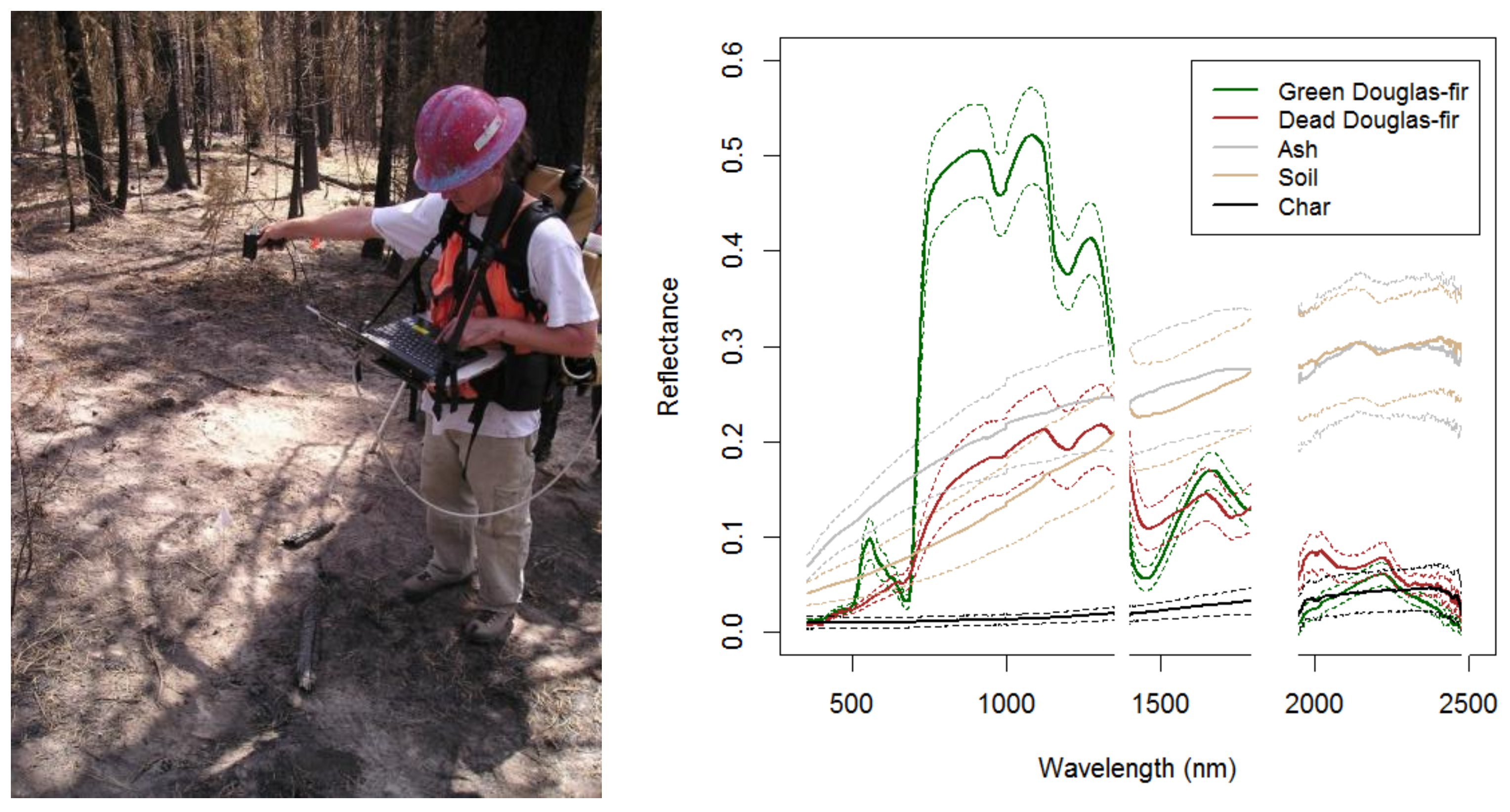
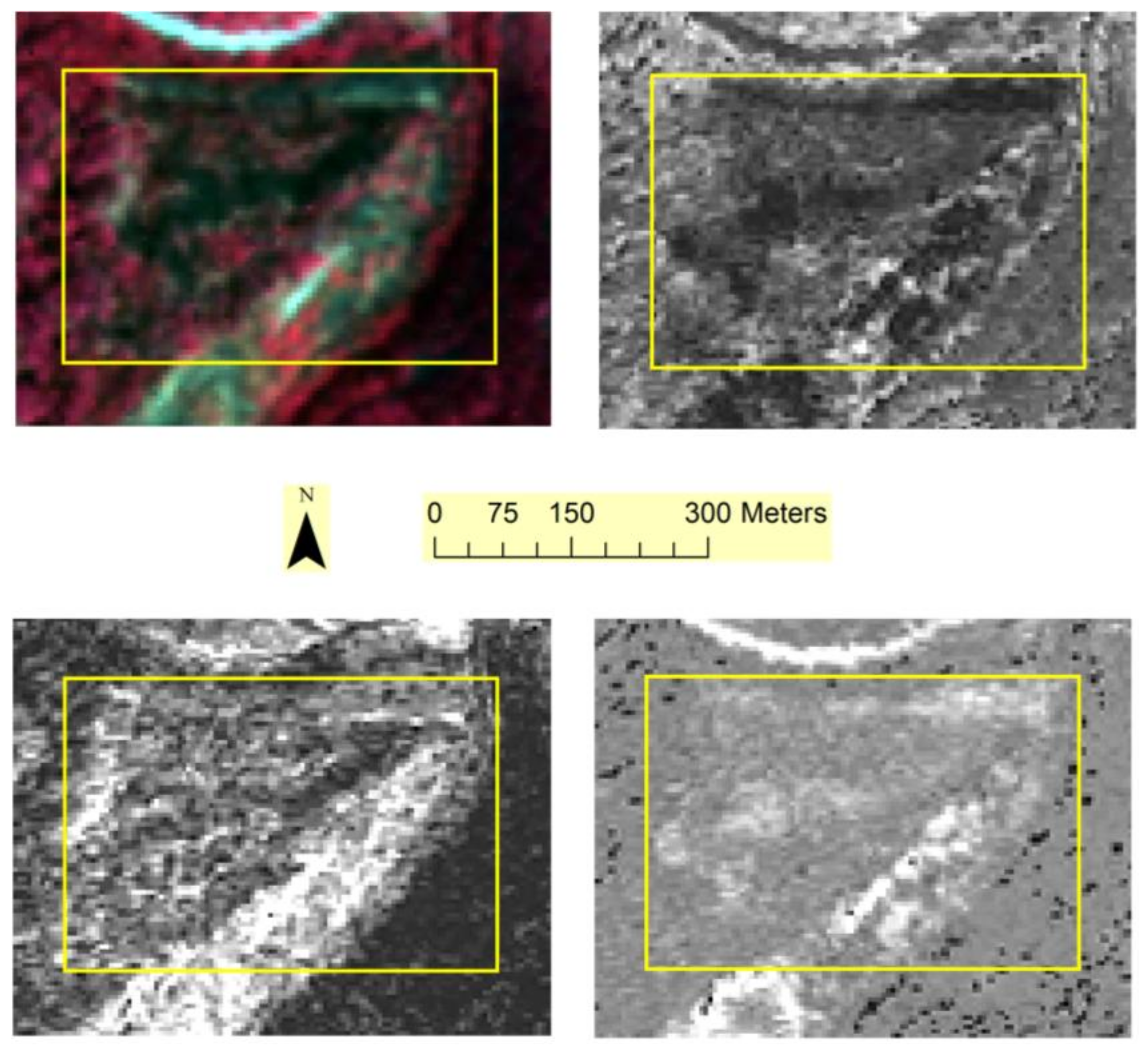
2.5. Hyperspectral Imagery

Radiometric corrections. Airborne hyperspectral image swaths of most of the Cooney Ridge wildfire were collected on 14 September 2003 with a Probe-1 whiskbroom sensor at a nominal ground resolution of 4.5 m. The 128 channels spanning 432–2512 nm with bandwidths of 11–19 nm were radiometrically corrected to apparent reflectance by the vendor (Earth Search Sciences Inc., Kalispell, MT, USA) using FLAASH (Fast Line-of-sight Atmospheric Analysis of Spectral Hypercubes) software (FLAASH Spectral Sciences, Inc., Burlington, MA, USA). The reflectance data were further refined using a Radiative Transfer Ground Calibration (RTGC) [31], followed by an Empirical Line Calibration (ELC) using field spectral reflectance data collected nearby on a bright gravel roadbed, to standardize atmospheric and illumination effects across all the image bands [32]. Bands between 1340–1480 nm and 1810–1970 nm were eliminated because of atmospheric water absorption, and another band at 2512 nm was removed for noise, leaving 119 bands for Multiple Endmember Spectral Mixture Analysis (MESMA).

Geometric corrections. The airborne image vendor supplied input geometry files for georeferencing hyperspectral image swaths, but the images remained distorted, so prior to extracting any image pixel values at fire effects subplot locations, the images were warped to a 1 m orthorectified base image collected by the National Agriculture Imagery Program (NAIP) on 20 July2009 (Figure 1). Delauney triangulation was employed to get an accurate match to the base image, as evidenced by how well roads and other local features matched the base image. Delauney triangulation requires a high density of ground control points (GCPs); there were 130 GCPs in the case of the flightline that imaged the experimental burn area. The 1 m resolution warped image outputs were subsequently resampled to 5 m resolution using cubic convolution radiometric resampling.

Multiple Endmember Spectral Mixture Analysis (MESMA). The reflectance signal recorded in an image is a function of the distinct reflectance spectra (Figure 3) of the different component materials comprising the scene (Figure 4). Assuming that this mixing is a linear function of their relative proportions, the linear mixture model is defined as:

$$R_i={\displaystyle \sum }_{j=1}^n\left(R_{i,j}{f}_j\right)+e_i$$

(6)

where R_i is the spectral reflectance of the ith spectral band of a pixel, R_i,j is the spectral reflectance of endmember j in band i, f_j is the fractional cover of endmember j, and e_i is the error in band i. MESMA uses this same linear model as other SMA methods, but allows the endmembers to vary between pixels rather than adhere to the stricter SMA constraint that each pixel contain the same endmembers [33]. MESMA also allows for variation within the same material, such as different tree species representing green vegetation. MESMA code is part of VIPER (Visualization and Image Processing for Environmental Research) Tools (VIPER Tools, Santa Barbara, CA, USA), which has an iterative endmember selection process built in, such that the most representative endmembers are selected [34,35]. VIPER Tools are implemented as an add-on to ENVI image processing software (Harris Geospatial Solutions, Broomfield, CO, USA).

Reference endmember reflectance spectra (Figure 3) of all surface cover materials (Figure 4) were collected on site with a field spectroradiometer (ASD Pro-FR) at the time of fire effects characterization (21 September 2003). The spectroradiometer collects spectra in 2050 channels with 1 nm bandwidths spanning 350–2500 nm. Reference endmember bundles of green needle, dead needle, charred wood, ash, and mineral soil spectra (Figure 3 and Figure 4) were used to unmix all of the hyperspectral image swaths collected over the Cooney Ridge wildfire [5], and the experimental burnout area was subsequently subset from the MESMA image outputs for this study.

2.6. Combining Active and Post-Fire Measurements to Predict Fire Effects

The airborne LWIR derived FRED images had ~4.5 m resolution pixels that were neither exactly square nor aligned to the hyperspectral image-derived MESMA images collected independently. The FRED images were therefore nearest-neighbor resampled to the same 5 m × 5 m resolution and pixel alignment as the MESMA images and with a common extent of 63 rows × 93 columns (5859 pixels) that fully imaged the burnout area, which equates to a 315 m × 465 m analysis area (14.65 ha; yellow rectangle in Figure 1). The FRED and MESMA images were considered as candidate predictor variables in multiple linear regression models for predicting percent cover of litter and mineral soil measured at the 195 subplots. A best subsets procedure was used to select the best predictor variable combination based on the lowest Akaike Information Criterion (AIC) [36], with candidate models ranging from univariate to including all predictors. Spatial simultaneous autoregressive models [37,38] were used to make use of the spatial autocorrelation between the nested field subplots, to increase predictive power over an aspatial multiple linear regression model [39]. Residual autocorrelation was assessed using Moran’s I and Geary’s C statistics. Analysis of variance (ANOVA) was used to compare the two models and assess whether the spatial model significantly increased variance explained on the basis of the log likelihood. All statistical analyses were done using R software [40].

3. Results

3.1. Tree Mortality

The experimental burnout operation on 3 September 2003 began at approximately 13:00 MDT, but the fire did not enter the fuel plot until approximately 15:45. Fuel moistures were much lower than would be permitted for a typical prescribed fire (1 h, 16%; 10 h, 15%; 100 h, 13%; 1000 h, 48%). Torching behavior was observed, particularly of subalpine firs (Figure 5), and scorch heights exceeded the 26 m tall trees. The fire killed all the mature subalpine fir and Douglas fir trees in the fuel plot, while a single western larch was damaged but survived (

Table 2. Pre-fire and post-fire measurements of the trees tallied in the fuel plot. Pre-fire data were collected on 3 September 2003, and post-fire data on 11 September 2003.

Species	Sample Event	Live Trees (ha−1)	Live Basal Area (m2 ha−1)	Avg. Live Crown Base Height (m)	Avg. Height (m)	QMD (cm)	Saplings (ha−1)	Seedlings (ha−1)	Total Live (ha−1)	Snags (ha−1)
Subalpine fir	Pre	98.8	2.8	1.6	16.5	18.9	197.7	3459.4	3755.9	0
	Post	0	0	0	0	0	0	741.3	741.3	98.8
	Difference	−98.8	−2.8	−1.6	−16.5	−18.9	−197.7	−2718.1	−3014.6	98.8
Western larch	Pre	24.7	1.6	4.3	25.9	29	0	0	24.7	0
	Post	24.7	1.6		25.9	29	0	0	24.7	0
	Difference	0	0	−4.3	0	0	0	0	0	0
Engelmann spruce	Pre	0	0	0	0	0	49.4	2223.9	2273.3	0
	Post	0	0	0	0	0	0	0	0	0
	Difference	0	0	0	0	0	−49.4	−2223.9	−2273.3	0
Douglas fir	Pre	49.4	2.6	1.8	17.5	26	24.7	3459.4	3533.5	0
	Post	0	0	0	0	0	0	741.3	741.3	49.4
	Difference	−49.4	−2.6	−1.8	−17.5	−26	−24.7	−2718.1	−2792.2	49.4
Total Trees	Pre	173	7	2	18.1	22.7	271.8	9142.7	9587.5	0
	Post	24.7	1.6	4.3	25.9	29	0	1482.6	1507.3	148.3
	Difference	−148.3	−5.4	2.3	7.8	6.3	−271.8	−7660.1	−8080.2	148.3

). All saplings of subalpine fir, Douglas fir, and Engelmann spruce (Picea engelmannii) were killed by the fire, and seedlings of the same three species were reduced by approximately 84%.

3.2. Fuel Loading and Consumption

The fire consumed 82% of the dead and downed woody fuel and 96% of the total forest floor fuel load [41].

Table 3. Forest floor fuel loadings in 2003 at the single fuel plot and in 2013 at six fire effects plots, enabling the calculation of the mean (SD).

Fuel Fraction	2003 (Fuel Plot)				2013 (Fuel Plot)	2013 (Fire Effects Plots)
	Pre-Fire (kg m−2)	Post-Fire (kg m−2)	Difference (kg m−2)	Consumption (%)	(kg m−2)	(kg m−2)
1000 h	1.513	0.000	−1.513	100.00	NA	2.30 1
100 h	0.170	0.170	0.000	0.00	0.00	1.38 (1.81)
10 h	0.518	0.208	−0.309	59.74	0.02	0.68 (0.75)
1 h	0.016	0.013	−0.002	14.29	0.05	0.22 (0.24)
Litter	3.699	0.135	−3.564	96.36	0.53	0.47 (0.18)
Duff	0.000	0.000	0.000	0.00	1.27	1.20 (0.38)
Total	5.916	0.527	−5.389	91.10	1.87	6.25

¹ In 2013, 1000 h fuels were only estimated at the center fire effects plot (Figure 3), 60 m upslope from the fuel plot.

shows the consumption of the separate forest floor components in the fuel plot, which burned at a low-moderate severity relative to the mixed fire severities observed across the site (Figure 6) and across the Cooney Ridge Fire as a whole [42]. A fuel load consumption of 5.4 kg m⁻² from the field surveys is expected to produce a FRED of 11.9 MJ m⁻² [26]. If we factor in the previously reported fuel moistures, converted to gravimetric water contents and weighted by the percent consumption estimates reported in Table 3 for the different fuel components, then the expected FRED is reduced to 10.9 MJ m⁻² [23].

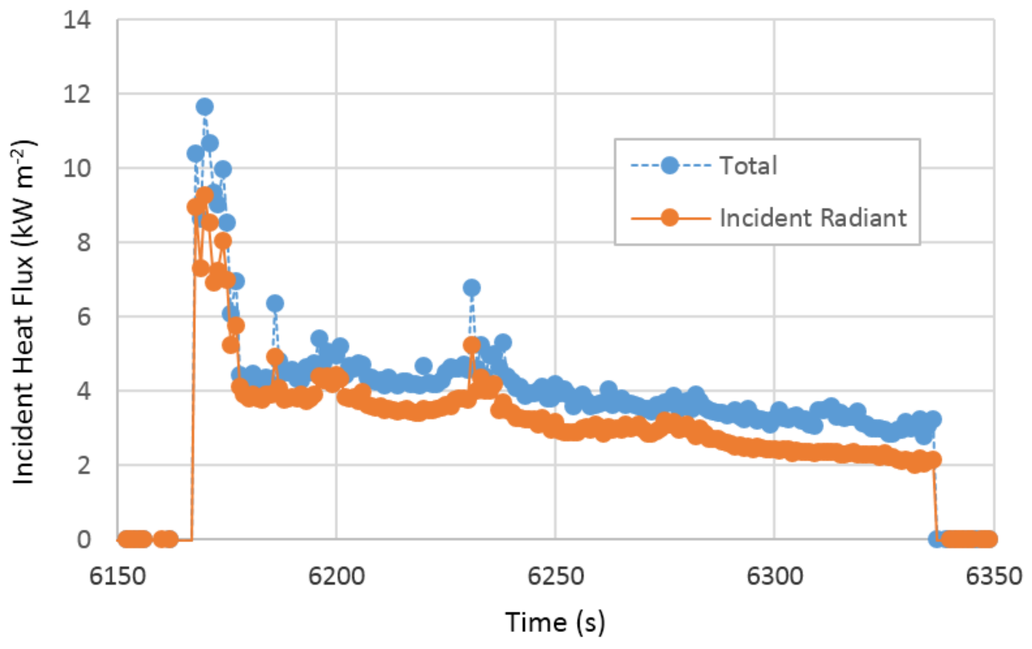
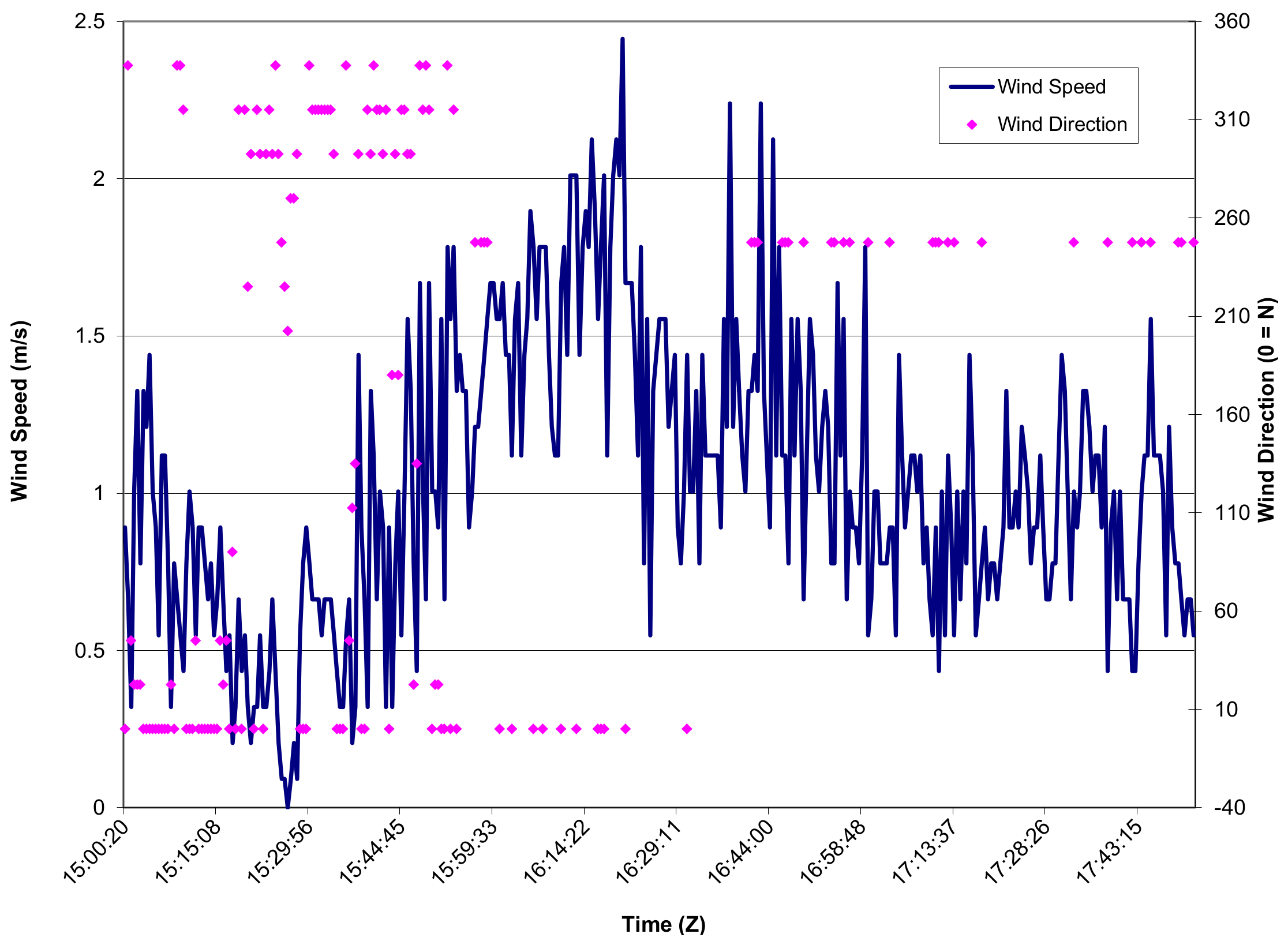
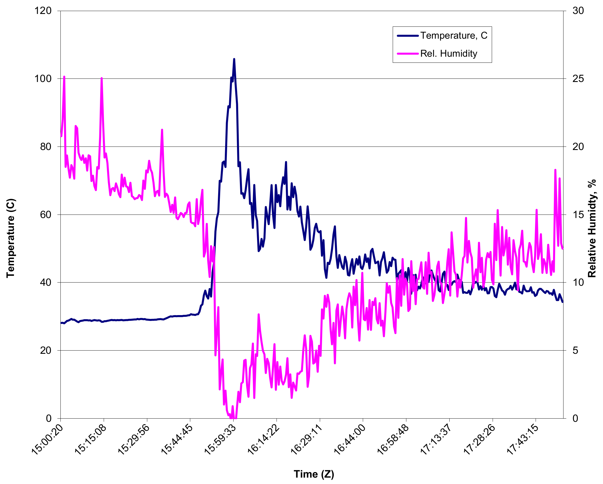
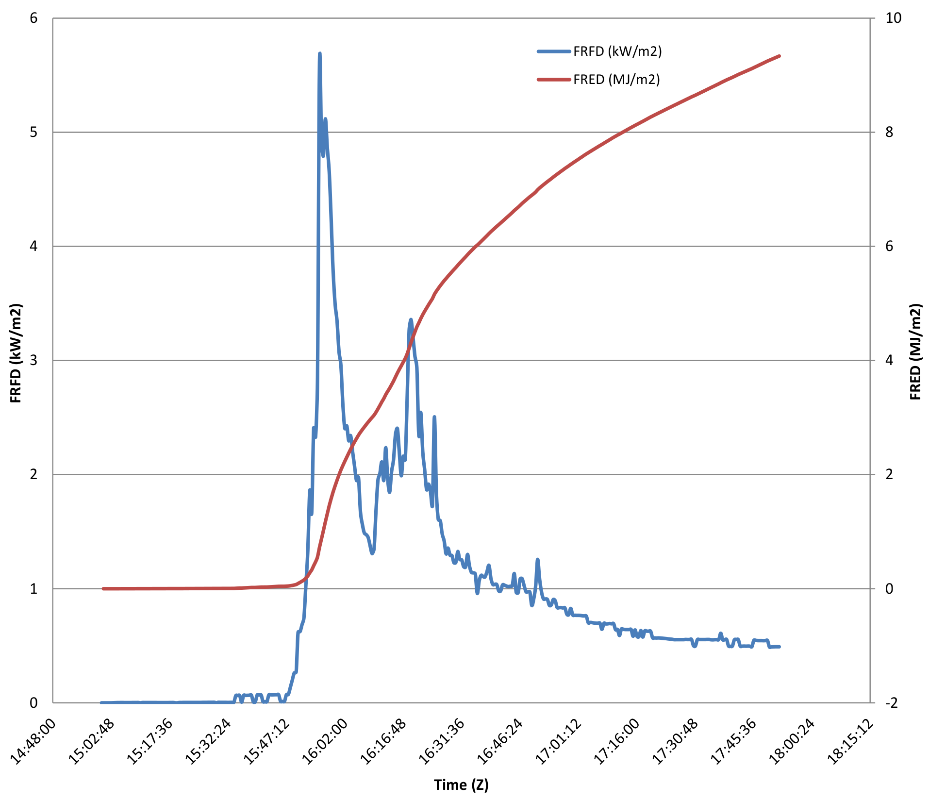
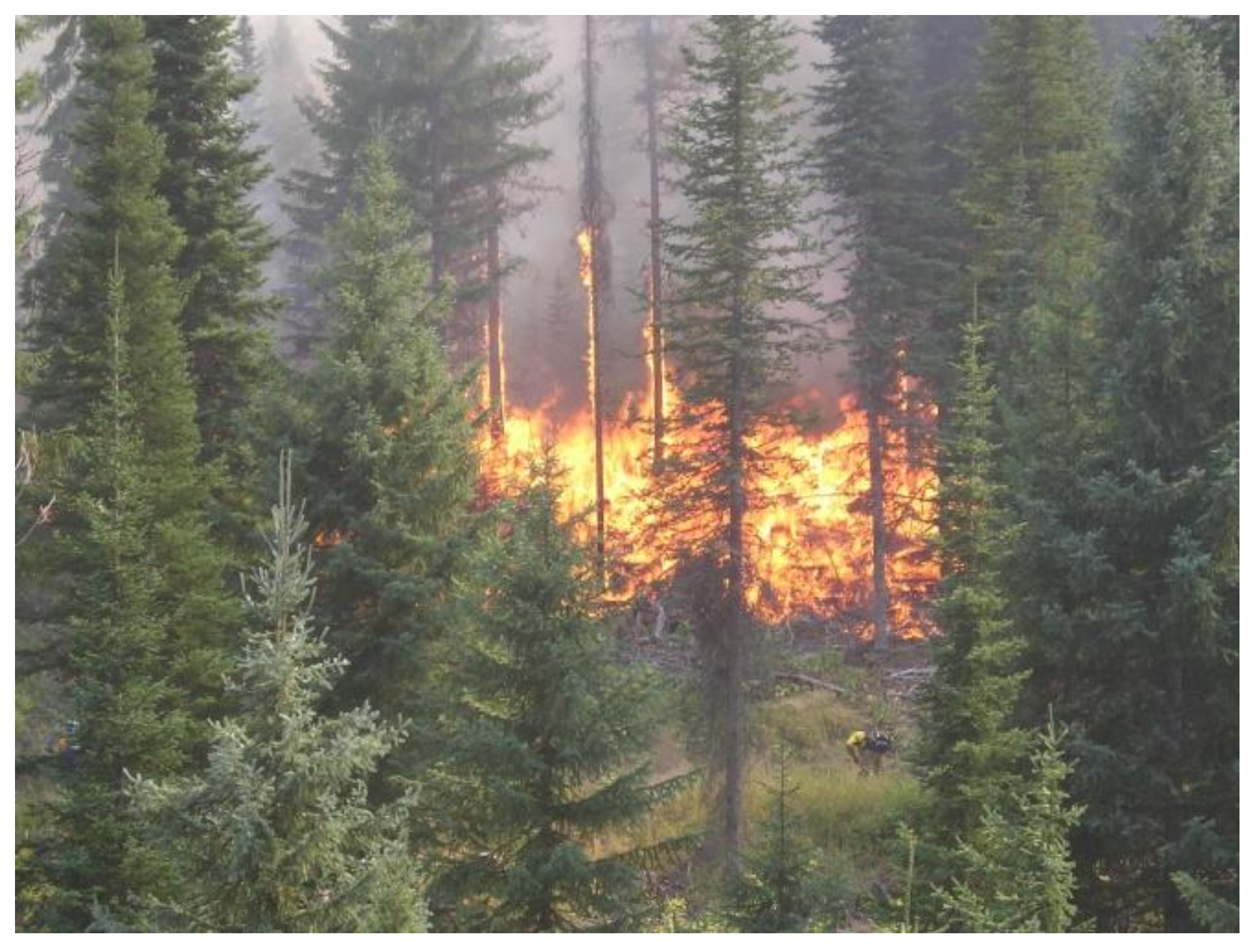
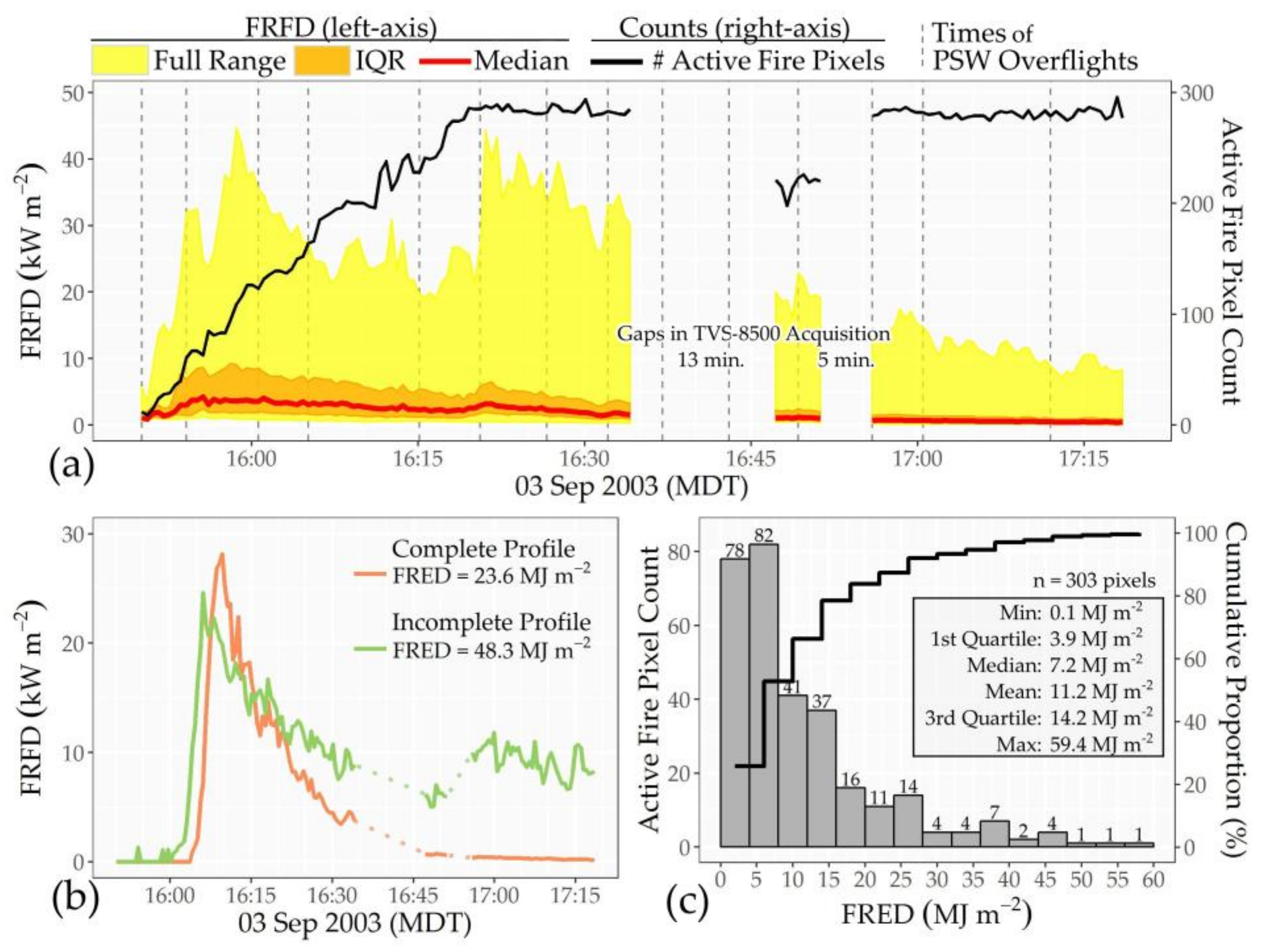
3.3. In Situ Heat Flux and Weather

Although the datalogger in the FBP located on the west side of the fuel plot failed to record, in situ measurements of total and radiant heat flux were successfully recorded at 1 Hz by the FBP on the east side of the fuel plot (Figure 1). The initial flaming combustion phase lasted 10 s, and, although the FBP radiometers are side-looking and captured the heating of opposing tree stems, the field of view (FOV) likely also contained surface fuels as well as the forest floor as evidenced by a slowly decaying heat release rate that lasted 2 min 38 s, indicative of a smoldering combustion phase with some residual flames. The total incident heat flux peaked at 11.7 kW m⁻² just 3 s after entering the sensor’s field of view (Figure 7). The total heat flux during the smoldering phase dropped from ~4.4 kW m⁻² to ~3.0 kW m⁻², while FRFD dropped from ~3.9 kW m⁻² to ~2.2 kW m⁻² (Figure 7). Thus, an estimated radiant fraction of ~0.8 was nearly constant during the record of observation. This is a much higher radiant fraction than typically reported [23,26,43,44]. Estimated FRED from the eastern FBP reached 0.57 MJ m⁻² before the radiometer stopped responding.

Although the western AES was immolated in the fire (Figure 8a,b), weather data and heat flux were successfully recorded at the AES deployed east of the fuel plot (Figure 8c). The increase in wind speed at ~15:30 was the first variable to presage the arrival of the fire front (Figure 9). At ~15:50, the wind direction shifted from the NW to the WSW (Figure 9), and the air temperature and relative humidity reached their extremes (Figure 10). A peak FRFD of almost 6 kW m⁻² occurred at ~15:55, about 5 min after the fire first entered the FOV, followed by a cooling phase that lasted longer than 2 h, during which the datalogger stopped recording. Integrating the FRFD profile over the 2.8 h record yielded a FRED estimate of 9.3 MJ m⁻² (Figure 11).

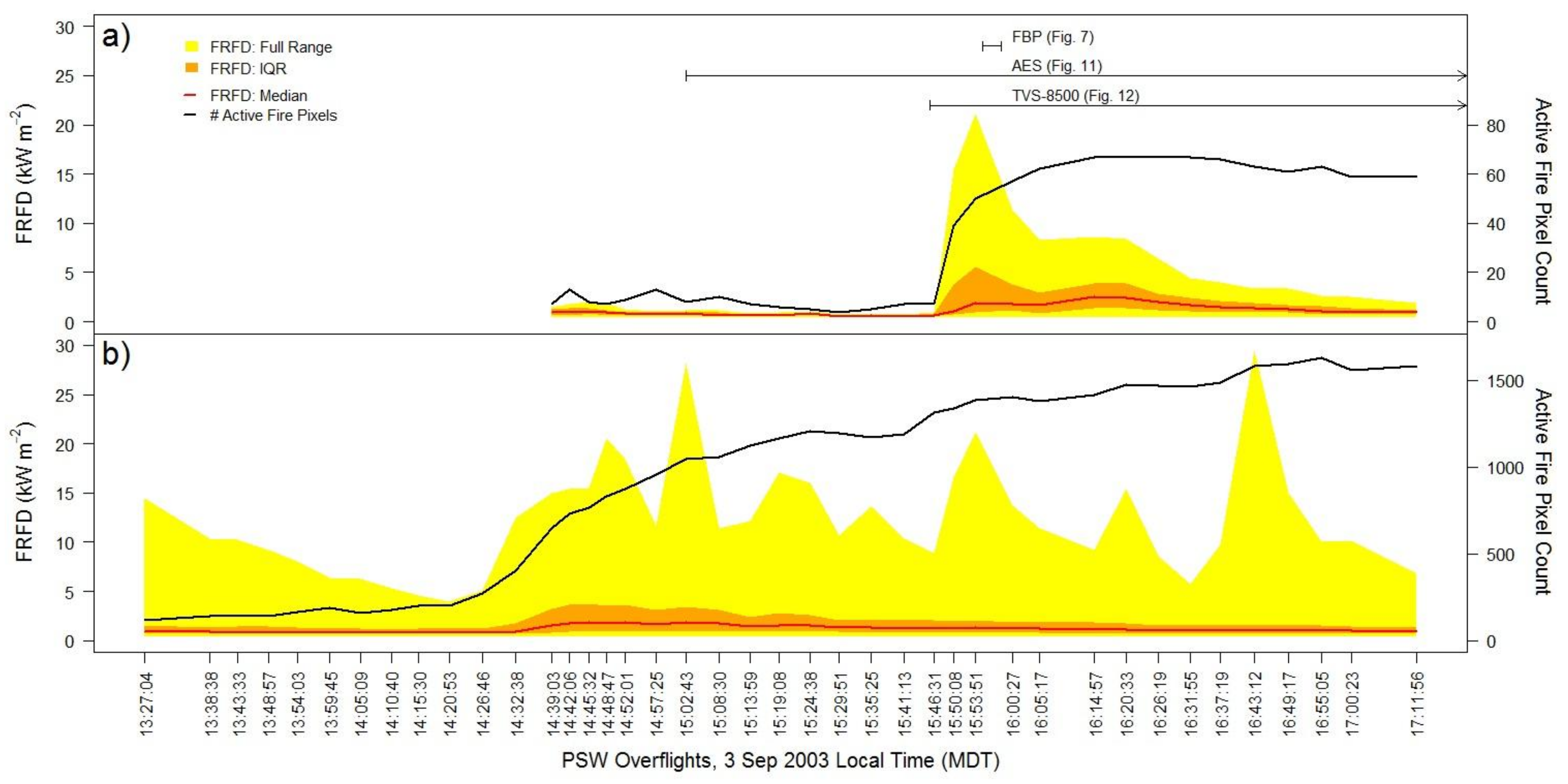
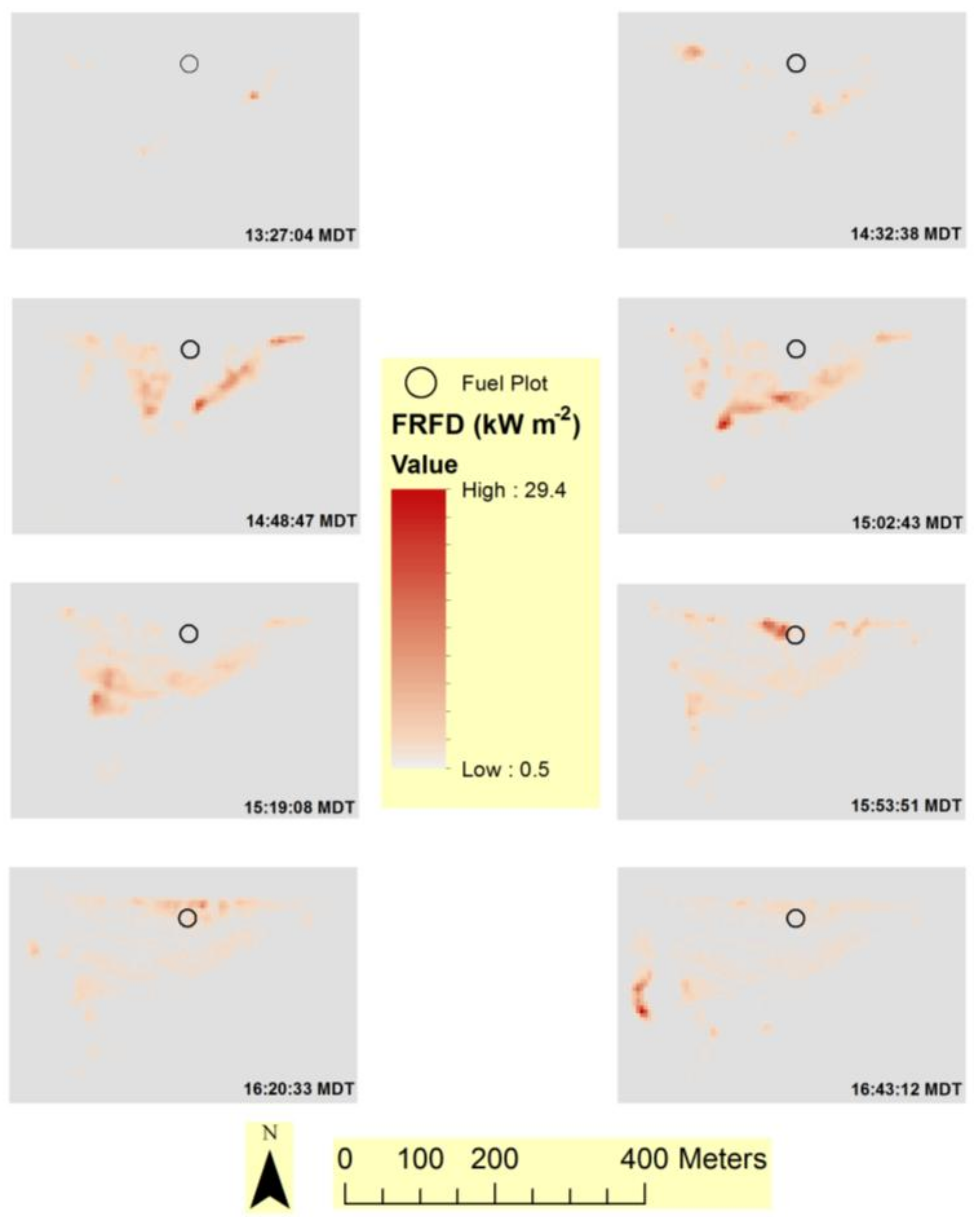
3.4. Thermal Infrared Imaging

Ground-based. The ground-based, low-oblique viewing MIR camera provided a third source of FRFD observations for a portion of the fuel plot (54%) not obscured by the two tree crowns in the foreground. Image collection commenced when the fire entered the fuel plot and began triggering active fire pixels (Figure 12a). FRFD calculated by Equation (2) used an ambient background temperature of 300 K. The minimum radiant heat flux measured for any individual pixel ranged from 0.1 to 0.9 kW m⁻², corresponding to the dynamic lower detection threshold, and a maximum per-pixel value of 44.8 kW m⁻² was recorded at 15:58. At no time did any thermal pixel in the fuel plot saturate, and the saturation rate outside of the fuel plot was less than 0.01%. The area-weighted average radiant heat flux emitted by the fire within the fuel plot reached a maximum of 6.2 kW m⁻² at 15:58. After the peak heat flux, the fire continued to spread for another ~20 min when, at 16:18, there was a small flare-up, and all pixels in the fuel plot visible from the low-oblique vantage point were ignited. Although data collection continued for another hour, not all fire activity in the fuel plot fully extinguished (Figure 12b). At 17:18, most pixels in the fuel plot visible with the TVS-8500 were warm enough to breach the dynamic detection threshold, however the majority of these active fire pixels were likely composed of cooling materials that emitted very little radiant heat. Nevertheless, 10% of the active fire pixels detected by the TVS-8500 at the end of the observations had FRFD values greater than 2.0 kW m⁻², a reasonable threshold at this spatial resolution to assume that sub-pixel combustion had not completely ceased.

Integrating the temporal profiles of FRFD for all 303 active fire pixels yielded a map of FRED for 54% of the fuel plot visible from the low-oblique vantage point. The distribution of the radiant heat per area (Figure 12c) is heavily right-skewed, ranging from 0.1 to 59.4 MJ m⁻², with half of the pixels below 7.2 MJ m⁻², indicating the spatial heterogeneity of the fire’s reaction intensity and/or residence time. Though unaffected by saturation, the distribution in Figure 12c is slightly misshaped because of the few incomplete observations of still burning materials (Figure 12b). Overall, the area-averaged FRED for the portion of the fuel plot visible in the low-oblique imagery was 11.2 MJ m⁻².

Airborne. The airborne system provided a time series of fire observations across the entire study area at fairly consistent intervals and over a longer period than the other sensors (Figure 13). An ambient background temperature of 300 K was used to estimate FRFD by Equation (4), on the basis of two considerations. First, brightness temperatures in an unburned, 13 × 9 pixel area situated in the forested, southeast corner of the scene ranged from 288 K to 302 K in the 42-image time series, with a mean of 297.6 K and a median of 296.0 K. Second, 300 K equates to 26.85 °C, closely matching the air temperature recorded by the AES (Figure 10).

The airborne imager captured 42 frames that completely covered the experimental fire area from 13:27 to 17:12. FRFD ranged from 0.5 to 29.4 MJ m⁻² over the period of airborne image collections, peaking in the fuel plot at 21.1 MJ m⁻² at ~15:54 (Figure 13).

Maps of FRFD from eight airborne images acquired when FRFD was peaking are shown in Figure 14. Ignition lines for backing fires were lit upslope of the fuel plot at about 13:15 (Figure 1). At the 13:27 start of the time series (Figure 13), the fire progression (with torching behavior) was most active >100 m upslope (SW and SE) of the fuel plot (Figure 14). Meanwhile, a lower intensity surface fire persisted immediately upslope (south) of the fuel plot and about ~50 m south of the active fire instruments (Figure 1) from ~14:40 until ~15:45. Because the fire did not back farther downslope into the fuel plot, perhaps because of pre-fire trampling of fine fuels in this vicinity during fuel sampling and equipment set up, fuels were hand-ignited for a head fire downslope (north) of the fuel plot starting at 15:45 (Figure 1). This presumably caused the local wind shift recorded at this time (Figure 9). Flaming combustion continued until ~17:15, and smoldering combustion continued beyond the measurement periods of the various sensors (Figure 7, Figure 11, Figure 12 and Figure 13). These observations were corroborated by personnel on the fire line.

Figure 15 illustrates estimated FRED integrated at each pixel over the FRFD time series (n = 42) by Equation (5). FRED ranged from 0.5 to 38.4 MJ m⁻² in the active fire pixels within the entire study area (Figure 13b), and mean FRED was 11.8 (s.d. 6.8) MJ m⁻² (Figure 15). Considering only the 68 FRED pixels within 23 m of the fuel plot center (100% active fire pixels), thus encompassing not just the fuel plot but also the FBP and AES active fire instruments (Figure 13a), FRED ranged from 0.9 to 27.2 MJ m⁻², and mean FRED was 10.1 (s.d. 5.5) MJ m⁻².

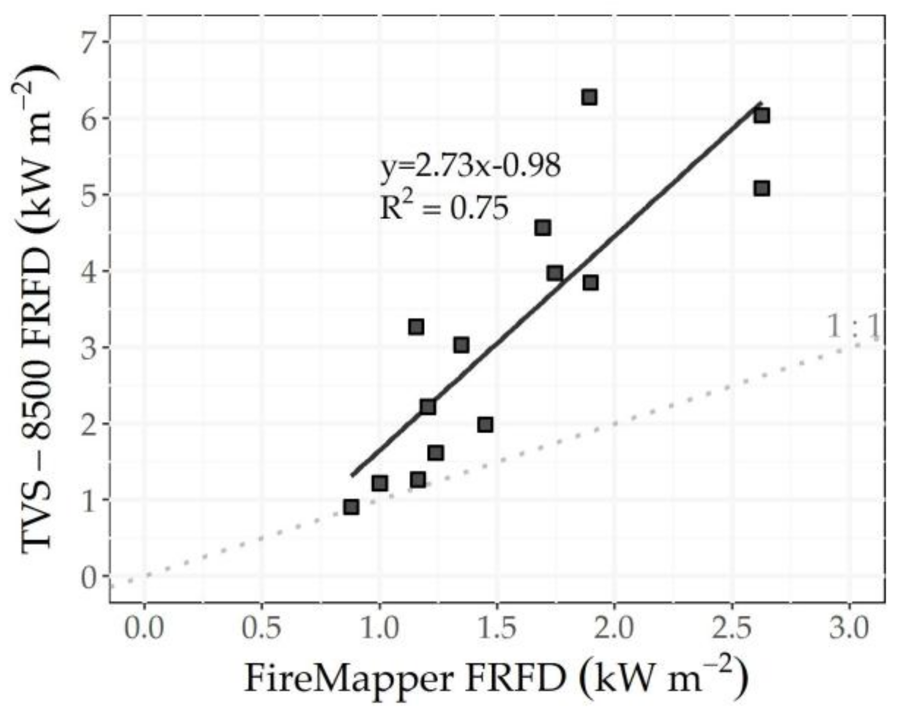
3.5. Multi-Scale Comparisons of Heat Flux Measurements

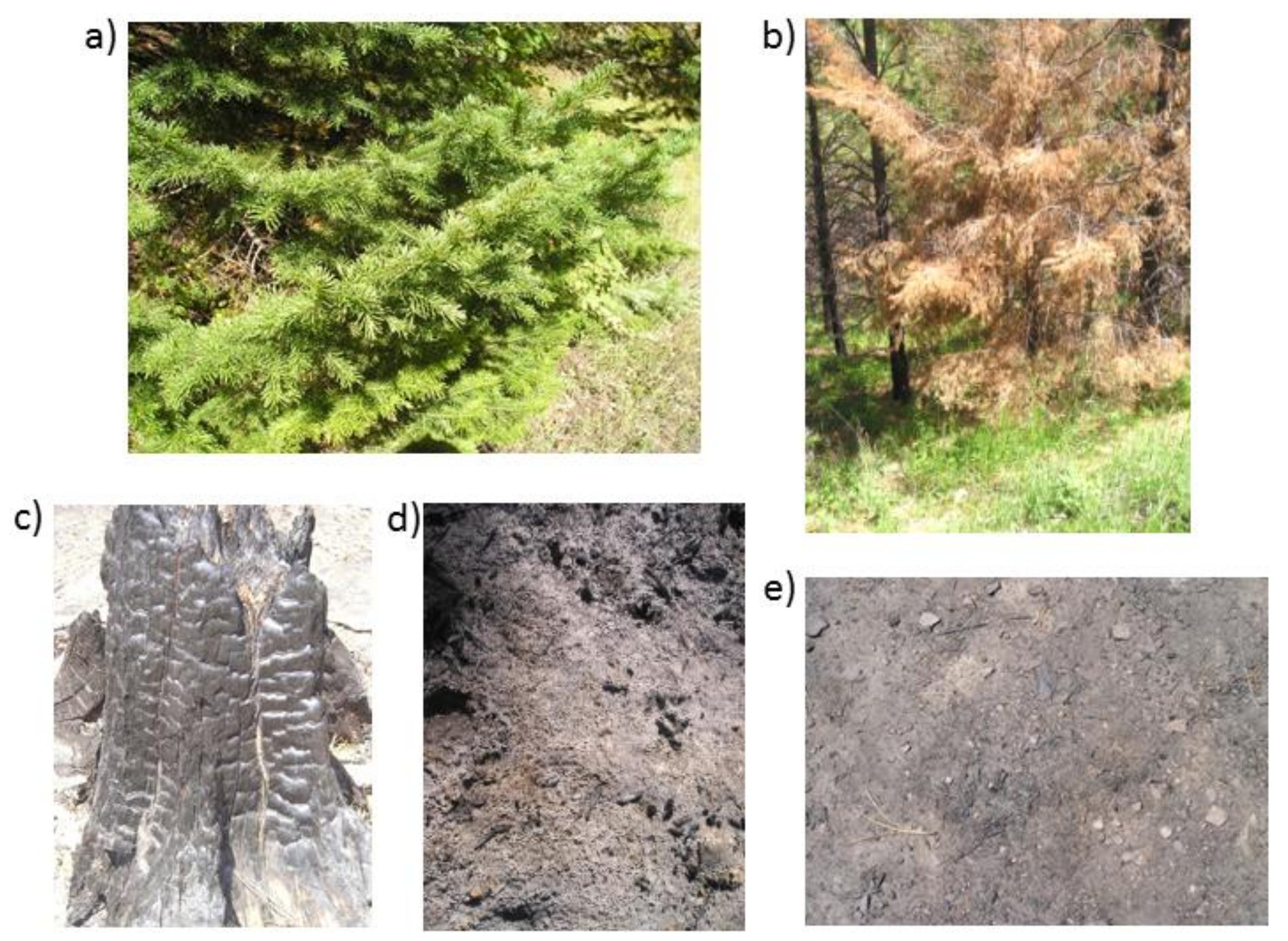
Because of our inadequate ability to identify what portion of the fuel plot was contained in the field of view of the FBP and AES radiometers, it is inadvisable to compare measurements from these two sensors with each other or with heat flux estimates derived from the ground-based or airborne infrared imagery. Instead, comparisons are limited here to the two sequences of georegistered images collected with the TVS-8500 and the FireMapper. Although georegistration errors prohibit per-pixel comparisons, the uncertainties in the pixel locations were mitigated by spatially averaging the estimates of FRFD and FRED over the entire fuel plot. Since 54% of the fuel plot was obscured in the low-oblique imagery by two tree crowns in the foreground, it is assumed that measurements in the visible portion of the fuel plot are representative of the hidden area behind the tree crowns.

On an instantaneous basis, estimates of the average FRFD over the fuel plot derived from the low-oblique MIR images and the nadir-looking LWIR images were strongly correlated (R² = 0.75), with the former always being higher (Figure 16). Despite the correlation, the response of the TVS-8500 and the FireMapper to varying thermal distributions and active fire sizes in the fuel plot was not constant. Sensor-to-sensor ratios (TVS-8500: FireMapper) of heat flux estimates ranged from 1.06 to 3.32, with estimates tending to agree more closely at lower values of FRFD. Consequently, differences in the spatially averaged FRED over the fuel consumption plot (11.2 MJ m⁻² from the TVS-8500 and 7.12 MJ m⁻² from the FireMapper) are primarily attributed to observations collected during periods of increased fire behavior.

3.6. Fire Effects

The immediate post-fire hyperspectral image of the experimental fire area and three derived MESMA images of estimated cover fractions are shown in Figure 17. These three MESMA images are not absolute measures of in situ ground cover, but discrete estimations of subpixel ground cover fractions that are distinct spectrally and spatially (Figure 17) across many pixels, as evidenced by low Pearson correlations: −0.52 (soil vs. green), −0.53 (soil vs. NPV), and r = 0.15 (green vs. NPV). Ash and char endmembers also were initially considered, but preliminary inspection of these endmember images revealed spectral confusion with soil and shade, respectively, which is also apparent visually (Figure 3 and Figure 4). Therefore, ash and char cover fractions were dropped from further consideration in the predictive models.

The mean cover percentages of the ground cover component materials, as estimated ocularly in the field at 195 subplots, were 45.3% NPV, 49.8% mineral soil, and 4.9% ash (

Table 4. Mean (SD) overstory canopy closure, plant species richness, ground cover fractions, and litter/duff depths.

Post-Fire Measurement	2003 (n = 13 plots)	2004 (n = 6 plots)	2013 (n = 6 plots)
overstory canopy closure (%)	38.6 (14.1)	44.6 (28.0)	10.9 (9.6)
plant species richness (m−2)	0.0 (0.0)	5.5 (4.5)	12.5 (2.4)
plant cover (%) 1	0.0 (0.0)	46.7 (13.8)	82.5 (25.6)
green vegetation (%) 2	0.0 (0.0)	35.2 (17.3)	65.0 (14.0)
organic (%) 3	45.3 (21.7)	35.2 (12.4)	31.5 (11.4)
inorganic (%) 4	49.8 (21.0)	26.7 (20.9)	3.5 (5.8)
ash (%)	4.9 (3.8)	3.6 (4.3)	0.0 (0.0)
char (%) 5	77.8 (21.0)	35.1 (23.7)	9.9 (12.5)
litter (mm)	9.1 (4.1)	4.0 (3.6)	10.7 (4.0)
duff (mm)	20.3 (7.5)	17.5 (10.6)	11.3 (3.6)

¹ Green plant cover <1.37 m breast height summed for all species, allowing for vertical overlap; ² Green plant cover <1.37 m breast height, collapsed on to a plane (no vertical overlap); ³ Includes non-photosynthetic litter, downed woody debris, and stumps; ⁴ Includes soil and rock; ⁵ The green, organic, inorganic, and ash cover fractions are constrained to sum to unity, whereas char is not and represents the combined percentage of the organic and inorganic cover fractions that is charred.

). No green ground cover vegetation was encountered below breast height while characterizing the 13 fire effects plots immediately post-fire (Figure 15). At the center fire effects plot (Figure 6a), all trees were killed, and the tree crowns were characterized as 94% black (charred) and 6% brown (scorched). However, tree crowns in some other fire effects plots were either mostly scorched (Figure 6b) or mostly green (Figure 6c); thus, the fire severity varied between fire effects plots. Mean canopy closure measured with a spherical densiometer at the time of field plot characterization immediately post-fire was 38.6% (Table 4), with no differentiation between green and NPV components.

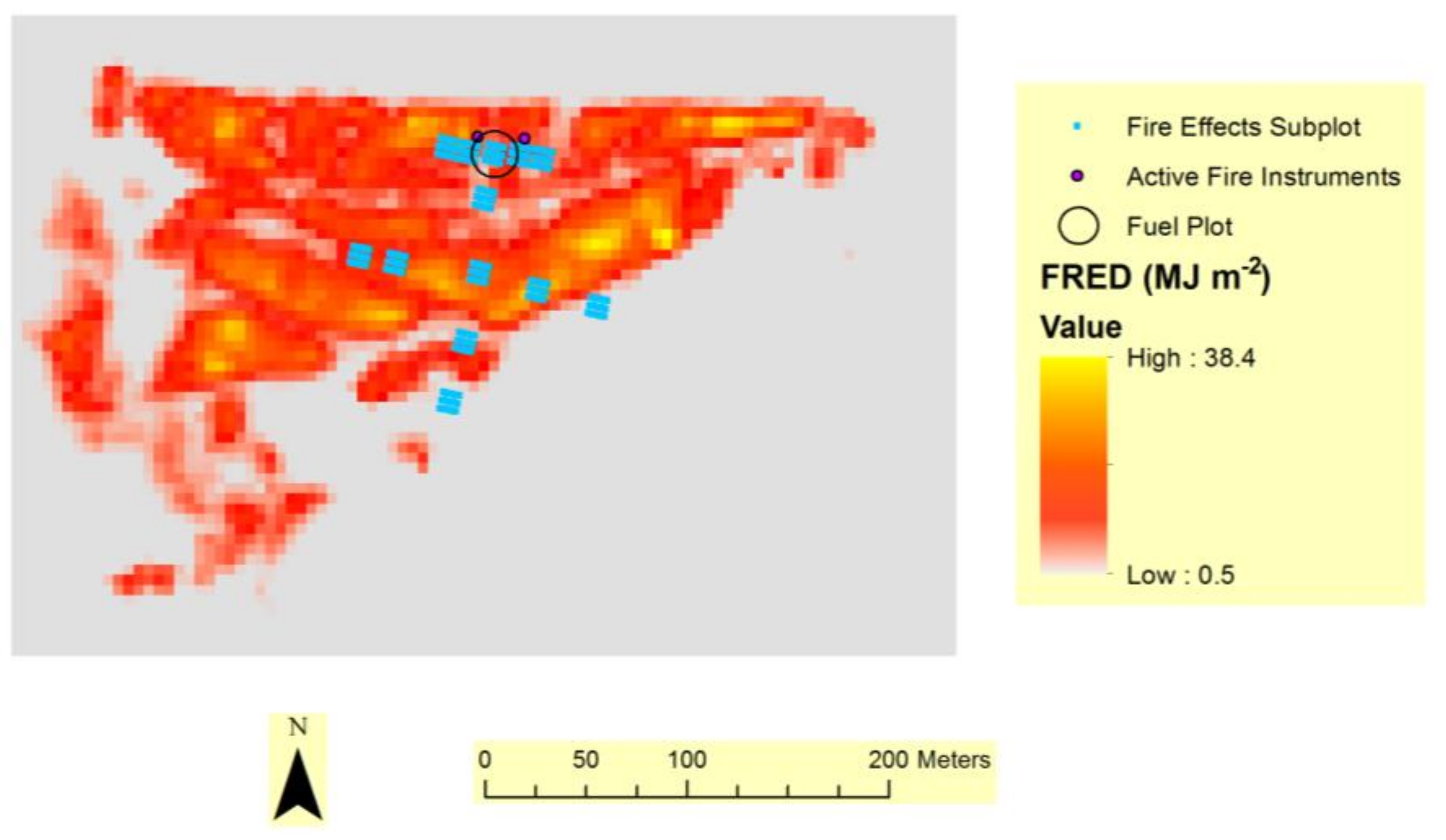
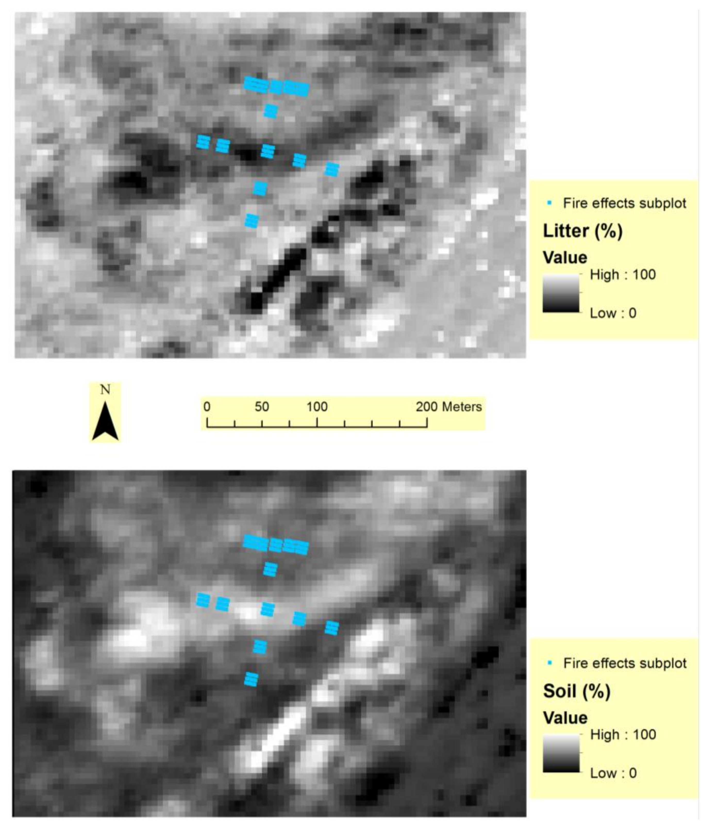
3.7. Active and Post-Fire Imagery Combined to Predict Fire Effects

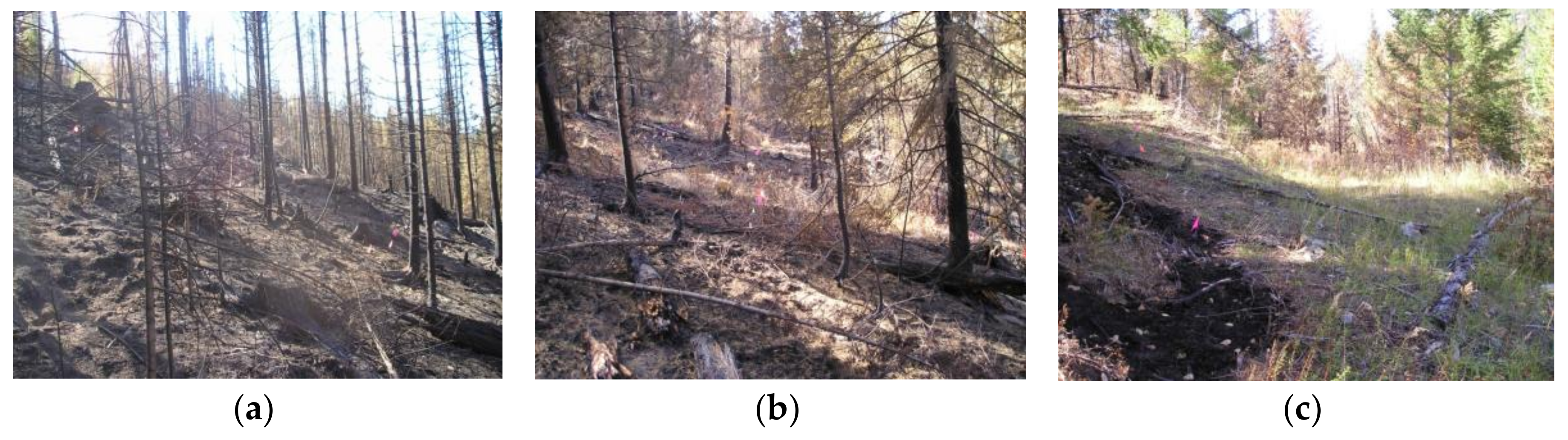
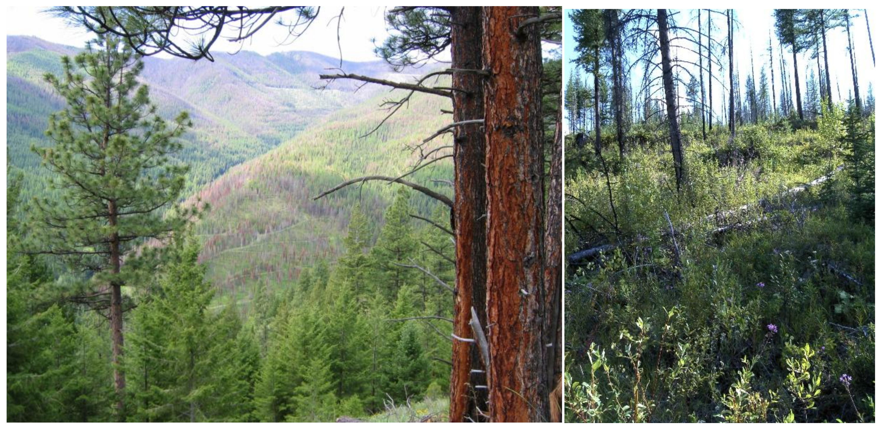
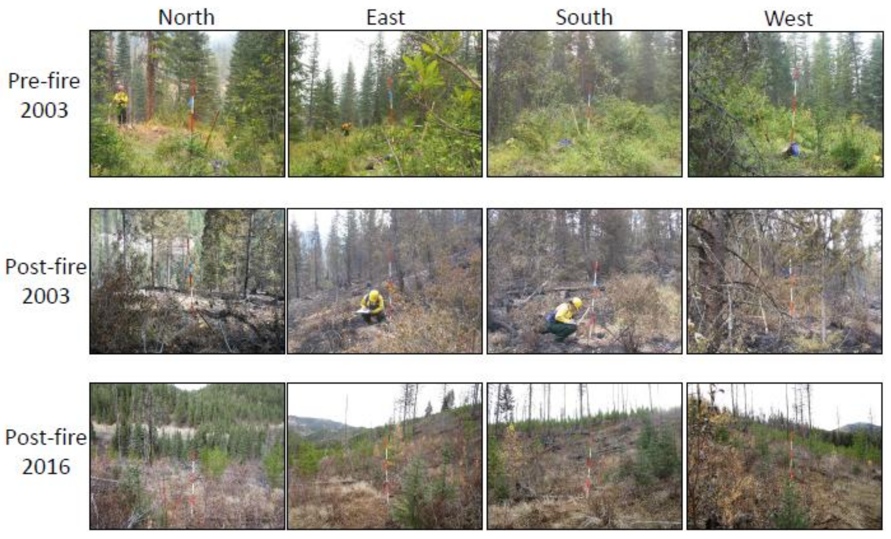
The lowest AIC among competing models resulted in three predictor variables, which produced the best subsets for multiple linear regression models predicting percent cover of litter and mineral soil. The selected variables for predicting both litter and mineral soil cover were airborne FRED first, followed by MESMA soil and then MESMA green (

Table 5. Descriptions of the models used to predict percent cover of A) litter and B) mineral soil. In each case, results include 1) linear regression and 2) spatial autoregression trend component; 3) results from an ANOVA comparing the aspatial and spatial models.

A) Litter Cover
1) Linear Regression	Estimate	SE	t value	Pr (>|t|)
(Intercept)	110.29	17.75	6.21	3.17 × 10−9
Airborne FRED	−1.21	0.31	−3.95	1.08 × 10−4
MESMA Soil	−274.92	80.21	−3.43	7.46 × 10−4
MESMA Green	96.48	48.95	1.97	0.05
Model Statistics:	RMSE = 28. 92; R2 = 0.30; p-value = 6.01 × 10−15
Residual Autocorrelation:	Moran’s I p-value = 0.0007; Geary’s C p-value = 0.0011
2) Spatial Autoregression	Estimate	SE	z value	Pr (>|z|)
(Intercept)	77.42	18.25	4.24	2.21 × 10−5
Airborne FRED	−0.81	0.29	−2.77	5.59 × 10−3
MESMA Soil	−210.62	76.50	−2.75	5.90 × 10−3
MESMA Green	47.56	46.76	1.02	0.31
Model Statistics:	RMSE = 27.35; R2 = 0.38; p-value = 6.62 × 10−5
Residual Autocorrelation:	Moran’s I p-value = 0.7723; Geary’s C p-value = 0.7757
3) ANOVA Comparison	df	AIC	logLik	L. Ratio	p-value
Linear Regression	5	1875.6	−932.78
Spatial Autoregression	6	1861.7	−924.82	15.916	6.62 × 10−5
B) Mineral Soil Cover
1) Linear Regression	Estimate	SE	t value	Pr (>|t|)
(Intercept)	−21.91	16.61	−1.32	0.19
Airborne FRED	1.17	0.29	4.09	6.49 × 10−5
MESMA Soil	306.01	75.06	4.08	6.69 × 10−5
MESMA Green	−80.91	45.81	−1.77	0.08
Model Statistics:	RMSE = 27.07; R2 = 0.33; p-value = 2.2 × 10−16
Residual Autocorrelation:	Moran’s I p-value = 0.0059; Geary’s C p-value = 0.0114
2) Spatial Autoregression	Estimate	SE	z value	Pr (>|z|)
(Intercept)	−24.99	15.86	−1.58	0.12
Airborne FRED	0.85	0.28	3.04	2.37 × 10−3
MESMA Soil	248.15	73.41	3.38	7.24 × 10−4
MESMA Green	−44.93	44.64	−1.01	0.31
Model Statistics:	RMSE = 26.08; R2 = 0.38; p-value = 1.02 × 10−3
Residual Autocorrelation:	Moran’s I p-value = 0.7422; Geary’s C p-value = 0.7728
3) ANOVA Comparison	df	AIC	logLik	L. Ratio	p-value
Linear Regression	5	1849.7	−919.86
Spatial Autoregression	6	1841.1	−914.56	10.595	1.13 × 10−3

). The measures of model fit (RMSE) and variance explained (R²) were slightly better for predicting mineral soil than litter cover (Table 5). Both models also had significantly autocorrelated residuals based on Moran’s I and Geary’s C statistics (Table 5), therefore invalidating the assumption of independent sample data. Fortunately, our spatially nested plot layout was actually designed to capture spatial dependence, which was exploited to increase predictive power using spatial simultaneous autoregressive models. Including the spatial signal in the models reduced the RMSE, increased the R², lowered the AIC value, and significantly increased the log likelihood compared to the aspatial linear regression models (Table 5). Moreover, the spatial autoregressive models removed autocorrelation from the residuals, on the basis of Moran’s I and Geary’s C statistics (Table 5). The spatial autoregressive models were then applied to map percent cover of litter and mineral soil. The fitted values illustrated in Figure 18 include the combined influence of both the linear trend (Table 5) and the spatial signal components, which comprise approximately two-thirds and one-third of the fit, respectively. Because NPV and soil were the two predominant cover fractions immediately post-fire, the mapped predictions are significantly, yet negatively, correlated (Pearson r = −0.98, p-value = 2.2 × 10⁻¹⁶).

Ash is a first-order fire effect and the direct result of combustion [45,46]. The Spearman rank correlation of post-fire ash to airborne FRED was significant (ρ = 0.34, p-value = 1.07 × 10⁻⁶), but not as strong as the correlation of mineral soil to airborne FRED (ρ = 0.50, p-value = 6.66 × 10⁻¹⁴), probably because there was 10 times as much mineral soil exposed (49.8%) as ash (4.9%) on site immediately post-fire (Table 4).

3.8. Site Recovery

When characterized immediately post-fire, white ash has been shown to correlate well with fuel consumption across a broad range of fuel types and loads [46]. Ash gets redistributed quickly by wind and water and integrated into the soil; however, and we believe this happened by the time of the post-fire hyperspectral image and field data collections, 11 and 18 days after the fire experiment, respectively. Nine months later, some ash (3.6%) was still visible through the new green vegetation regrowth (35.2%), which reduced the visible fractions of the non-photosynthetic organic material by 10.1%, inorganic material by 23.1%, and black char by 42.7% (Table 4). These trends continued to 2013, when green vegetation comprised 65% of ground cover, at the expense of the other ground materials (Table 4).

Many of the subalpine fir and Douglas fir trees that were either scorched or still green but girdled by the fire did not drop their needles until after the hyperspectral image was acquired, as was observed upon revisiting the site in July 2004, nine months after the burn. Many of these snags can be seen standing six years later in the 20 July 2009 high-resolution NAIP image (Figure 1). By the time of the ten-year post fire revisit (Figure 19), the majority of snags had fallen, reducing canopy closure by ~33% (Table 4) and increasing forest floor fuel loads, especially of the large 1000 h and 100 h fractions (Table 3).

The fire experiment reduced ground cover plant species richness to zero, with no green vegetation observed immediately post-fire at any of the 13 original plots (Table 4). Species richness across the experimental fire site increased from 5.5 species m⁻² in 2004 (pre-fire) to 12.5 species m⁻² in 2013 (Table 4). The fuel plot had the highest diversity of any plot, perhaps because it was at the base of the hillslope; species richness there increased from 9.4 species m⁻² in 2004 to 15.6 species m⁻² in 2013. The standard deviation in species richness between plots decreased from 4.5 species m⁻² one year post fire to 2.4 species m⁻² ten years post fire (Table 4).

In terms of tree species diversity, only Douglas fir seedlings were observed within the original fuel plot in 2004, but five species of conifer seedlings [Engelmann spruce, subalpine fir, western larch, lodgepole pine (Pinus contorta), and Douglas-fir] were observed in 2013. High light availability due to high tree mortality followed by the natural felling of most snags by 2013 promoted a major regeneration of willow (Salix spp.) and a minor regeneration of trembling aspen (Populus tremuloides) (Figure 19). Tree seedling density increased six-fold, from 0.16 seedling m⁻² in 2004 to 1.0 seedling m⁻² in 2013. There is no evidence of salvage logging or any other disturbance since the experiment, as most recently confirmed in a 2016 site revisit to complete a photopoint time series of the fuel plot (Figure 20).

4. Discussion

4.1. Fire Radiant Heat Flux

The goal of synergistically assimilating multi-scale measurements of radiant heat flux to quantitatively characterize wildland fire behavior and effects is hampered by several theoretical and technical issues. Over the course of the Cooney Ridge Fire Experiment and the Rapid Response project as a whole, we organized these issues into three themes broadly covering spectral, temporal, and spatial considerations (

Table 6. Theoretical and technical issues identified during the Cooney Ridge Fire Experiment and the Rapid Response project as a whole, organized by spectral, temporal, and spatial themes. Citations of relevant works associated with these issues are contained herein, whilst references to supporting figures can be found in the body of the Discussion.

Spectral Bandpass and Response:

The choice of method for converting a spectral radiance measurement into an estimate of the spectrally integrated radiant heat flux [25,27,48] depends on the sensor bandpass.

Sensors with different spectral bandpasses respond differently to the radiant heat emitted by flames, glowing fuel particles, and smoldering embers [49,50]. Therefore, estimates of FRFD and FRED are affected by the combustion phase at the time of observation as well as by the evolution of the combustion phases from ignition to extinction, respectively.

Most commercial and custom-built radiometers and thermal imaging systems operate at different wavelengths [51], making direct sensor-to-sensor comparisons difficult.

Converting “at-sensor” measurements to “at-ground” estimates of FRFD requires knowledge of the spectrally dependent transmissivity of the intervening clear air and smoke plume [52].

Temporal Resolution and Coverage:

Although the sampling frequencies should be commensurate with the fire phenomena of interest [53], different sensor arrangements have different minimum and maximum sampling rates due to, for example, aircraft turnaround times and storage capacity.

Numerically integrating FRFD profiles to estimate FRED assumes a constant trajectory of FRFD between consecutive observations, an assumption that becomes less valid for infrequent observations of dynamic fire behaviour [53].

Confident estimates of FRED require complete observations of the entire combustion profile from ignition to extinction, and failing to do so will result in low estimates of FRED.

If the complete combustion history is not observed, then sensor-to-sensor comparisons of FRED must be restricted to the same temporal integration limits.

Spatial Resolution, Coverage and Viewing Geometry:

Ground extents and ground cell resolutions are affected by a combination of the instrument’s optical specifications as well as the line-of-sight distance between the sensor and the target. In general, the finer spatial resolution offered by a ground-based sensor is offset by reduced spatial coverage [24].

Even if collocated, sensors oriented in different directions (e.g., horizontal versus nadir-looking) will have different ground footprints. Without knowing the exact ground footprint of two different sensors, it is impossible to fully explain or compare heat flux estimates.

Radiant and convective heating of unburned vegetation in adjacent ground cells confounds fire detection strategies, induces uncertainties in the active fire area, and artificially contributes to FRP.

Estimates of FRFD based solely on the brightness temperature measured in a single band will be lower than the fire’s true radiant reaction intensity unless the IFOV is completely filled [54].

Estimates of FRFD as performed here depend on the subpixel fraction occupied by the active fire [54]. Hence, a larger pixel will result in a lower FRFD when compared to a smaller pixel containing the exact same fire. Hence, sensor-to-sensor comparisons of FRFD depend on the ground resolution of each sensor.

The spatial dependence of FRFD on subpixel active fire area is mitigated when measurements are integrated over time. Although FRED is also calculated with respect to the full ground area of a pixel, the underlying assumption associated with FRED is that the full ground area of a pixel is burned over the lifetime of the fire. If the entire area inside a ground resolution cell burns, which is a likely assumption, then FRED represents the fire’s true heat per unit area.

The practical advantages of a low-oblique vantage point are offset by extreme view angles and potential obscuration of the fire due to vegetative cover in the foreground [24].

Aside from assuming that the fire is an isotropic emitter, calculating the radiant heat flux from different view angles assumes that pixel brightness temperatures are independent of the orientation of the fuels and the flame geometry (i.e., independent of the configuration factor between the hot objects and the detector). This assumption, however, is less valid at extreme observation angles [52,55].

The radiance emitted by a fire can also be attenuated by tree boles, branches, and foliage before it reaches the sensor. As with atmospheric transmittance, obscuration of the radiometric signal by vegetation is spatially dependent upon the amount, arrangement, and condition of the overstory and temporally dependent upon the consumption of vegetation itself.

).

One impediment to comparing sensor outputs is that each sensor operates in a different spectral band. If the broadband radiometers in the FBP and AES have a uniform spectral response and have been calibrated, then the conversion between the raw sensor signal and the spectrally integrated radiant heat flux over all wavelengths is a relatively straightforward procedure. In contrast, many narrow-band radiometers and most thermal imaging systems operate in specific atmospheric windows either between 3–5 μm (MIR) or 8–14 μm (LWIR) [47]. Although from a practical standpoint these atmospheric windows permit much of the fire emitted radiance to reach the sensor unattenuated, the challenges of estimating the spectrally integrated radiant heat flux from a spectral brightness temperature measurement has inspired the development of several novel approaches, namely, the emissivity-area product [44,48], a semi-empirical approach based on simulated sub-pixel thermal distributions [27], and the MIR radiance method [25]. Nevertheless, none of these approaches are completely resilient to the transient subpixel thermal distributions that fluctuate over time. For example, because of differences in their spectral bandpasses, the TVS-8500 and the FireMapper will respond differently depending on the combustion phase (i.e., flaming versus smoldering) and size of the active fire area observed. Consequently, the sensor-to-sensor comparisons of radiant heat flux (Figure 16) were influenced by the temporal evolution of the active fire area and thermal distributions—and thus the combustion history—within the fuel plot. Moreover, the atmospheric windows within which the TVS-8500 and FireMapper bandpasses reside are not perfectly transparent. As of yet, the spectrally dependent transmittance between the ground resolution cells and the ground-based and airborne imaging systems has not been taken into account. The path-integrated transmissivity has two components: a static component associated with the smoke-free atmosphere and a dynamic component associated with spatiotemporal variations in scattering and absorption by the smoke plume. Proper comparisons of radiant heat flux estimates will require that Equations (2) and (4) incorporate the spectrally, spatially, and temporally varying transmittance values as well as the line-of-sight distances between the sensor and fuel plot. Eliminating the spectral dependence on the measurement can be accomplished by using only instruments with the same bandpass, though this is likely impossible for a multi-scale campaign because of the technical requirements for each sensor package and platform.

Compared to fixed wing overflights, the use of a ground-based thermal imaging system offers improved temporal resolution (Figure 12a), which enables the near-continuous observation of high frequency fluctuations in fire behaviour. Using a time-discrete summation (Equation (3)) or the trapezoidal rule of numerical integration (Equation (5)) to estimate FRED assumes a constant FRFD—or a constant trajectory of FRFD—between consecutive observations, which becomes less valid for infrequent observations of dynamic fire behaviour. This is evidenced by fluctuations in the thermal distribution measured by the low-oblique camera at 30 s intervals between the airborne overpasses at ~5 min intervals (Figure 12a). More importantly, confident estimates of FRED require that the entire combustion profile from ignition to extinction be observed. Both the TVS-8500 and the FireMapper began imaging before the fire first entered the fuel plot, but active fire pixels persisted in the last images of each sequence indicating that combustion had not completely ceased. Figure 12b, for example, illustrates the FRFD profile for one pixel in the fuel consumption plot that was still burning when the low-oblique camera stopped collecting images. As such, the radiant heat emitted during the residual burning of fuels in this pixel remains unaccounted for. Failing to capture ignition and/or extinction will inevitable yield low estimates of FRED and ultimately affect field-derived relationships between FRED and fuel consumption, since pre- and post-burn surveys of fuel loads were conducted before ignition and after extinction. If the complete combustion history cannot be observed, then estimates of FRED should, at the very least, be compared on the basis of the same temporal integration limits. For this reason, estimates of FRED compared between the FireMapper and the TVS-8500 were obtained by setting the integration limits to the first and last times that both imaging systems simultaneously observed the fuel consumption plot (Figure 12a and Figure 16).

The FBP’s were oriented horizontally (i.e., parallel to the ground) to collect measurements of the incident radiant heat flux as if it were an object ahead of the fire front, for example a fuel particle or a human being. The intent of collecting airborne and low-oblique thermal images was to map the radiant heat flux and energy emitted from the fire. These are two different phenomena: irradiance versus exitance. For these reasons, the FBP measurements were not compared to the thermal imagery. Although the radiometer mounted on the AES was oriented to view the ground at 45°, we were unable to confidently identify the outline of the ground resolution cell because of the time constraints imposed by the advancing wildfire. Without knowing their exact ground footprints, it was not possible to confidently map the AES radiometer measurements onto the airborne or low-oblique imagery; hence, differences in radiant heat estimates from the AES radiometers cannot be fully explained nor compared to estimates derived from the thermal imagery. Moreover, it can be contended that the FRFD estimated from the FBP and AES radiometers is not meaningful anyway, since the values are based on the full area of the ground resolution cell. Instead, a proper calculation of FRFD from the in situ radiometers would require the retrieval of the sub-resolution active fire area. Likewise, for estimates derived from the FireMapper imagery. With a nominal ground resolution of 4.5 m, it is unlikely that the active fire area completely filled the IFOV of a FireMapper pixel, such as when the fire first entered the fuel plot. On the occasions when the active fire area is smaller than the pixel area, then FRFD will be underestimated. Because of larger pixel sizes, estimates of FRFD derived from the FireMapper imagery were consistently less than those derived from the TVS-8500 imagery with a nominal ground resolution of 0.8 m. Although sensor-to-sensor differences in the size of the IFOV’s interact with the temporal variability in the size of the active fire area to confound comparisons of FRFD on an instantaneous basis, these hindrances are mitigated when the measurements are integrated over time. FRED is also calculated with respect to the full ground area of a pixel, but the underlying assumption associated with FRED is that the full ground area of a pixel is burned over the lifetime of the fire. In this regard, sensor-to-sensor comparisons of FRED are less complicated by differences in spatial resolution.

The improved spatial resolution offered by a ground-based sensor arrangement is offset by the reduced spatial coverage and, with regard to the low-oblique vantage point, offset by extreme view angles and potential obscuration of the line-of-site due to vegetative cover in the foreground (Figure 19a). Aside from assuming that the fire is an isotropic emitter, calculating the radiant heat flux from different view angles assumes that the pixel brightness temperatures are independent of the orientation of the fuels and the flame geometry (i.e., independent of the configuration factor between the hot objects and the detector). This assumption, however, is less valid at extreme observation angles. In addition to the smoke plume and intervening clear atmosphere, the radiance emitted by a fire can also be attenuated by tree boles, branches, and foliage. As with atmospheric transmittance, obscuration of the radiometric signal by the vegetation is spatially dependent upon the structure of the overstory and temporally dependent upon the consumption of the vegetative cover itself.

From an image processing standpoint, the heating and cooling of the adjacent vegetation and overhead canopy simultaneously confounds the fire detection strategy and inadvertently contributes to FRP. Radiative contributions from warm, non-combusting vegetation should not be considered as FRP for two reasons. First, Equations (2) and (4) both assume that fire is an isotropic emitter; therefore, any radiative energy emitted by the fire and intercepted by the surrounding vegetation is already accounted for before it is either reflected [49,50] or absorbed and re-emitted. Second, the vegetation surrounding the fire is also heated by convection. If FRP is to be strictly interpreted as the rate of radiative energy released from the combustion zone, then including the radiative flux emitted by convectively heated vegetation would artificially increase the estimate of FRP. For this same reason, the radiative flux of the smoke plume immediately above the fire [56,57] should also be neglected in the measurement of FRP. In general, any additional radiance above the background that is not directly emitted from gaseous and solid combustion processes makes it difficult to discern active fire pixels—and thus estimate active fire area—and quantify FRP.

Addressing the aforementioned theoretical issues obviously requires filling knowledge gaps. For example, characterizing a sensor’s radiometric response to different subpixel fractions of flaming, glowing, and smoldering components, or determining the MIR and LWIR transmissivity of a smoke column can be accomplished in a laboratory. However, translating or applying laboratory results to field measurements to better understand landscape-level relationships between radiant heat release and fire effects comes with its own set of caveats and limitations. Hence, the problem of solving the radiant energy budget also requires a technical solution. Unfortunately, as of yet, there is no “one-size-fits-all” combination of instrument, data acquisition system, and mounting platform that provides consistent spectral, temporal, and spatial observations from a broad range of multi-scale deployment configurations. Consequently, different sensors must be selected on the basis of their ability to be deployed and perform at specific scales, which in turn makes it difficult to assimilate datasets of differing spectral, temporal, and spatial resolutions. To this day, more than a decade after the Cooney Ridge Fire Experiment, scientists are still struggling with the arduous challenge of assimilating multi-scale measurements collected with incongruous sensors [9,10,58,59,60].

4.2. Fire Effects

A previous analysis of landscape-level burn severity patterns in relation to pre-fire forest harvest patterns, conducted across the entire Cooney Ridge wildfire, did reveal significant relationships between stand-replacing harvest and stand-replacing fire disturbance patterns [42]. However, having only a single pre-fire fuel plot precluded us from examining pre-fire fuel distributions across the study site. If a vegetation and fuels monitoring network were already in place, it would be faster and easier to deploy fire behavior instruments wherever and whenever such plots occurred near an advancing wildfire.

Spatially distributed field plot and remotely sensed data were required to spatially model and map patterns in litter and mineral soil cover. FRED and the MESMA soil endmember had a similar ability to predict percent litter and mineral soil cover (Table 5), therefore either of the predictive maps in Figure 18 could be considered indicative of spatial variation in soil effects from the fire. While it is appealing to consider the FRED map a measure of heat dosage akin to fire severity [61], the airborne FRED measurements in this study convolved the heat release of all fuel components, including from torching tree crowns, thus combining the canopy and surface fuel components of combustion in the FRED map; however, it is surface fuel combustion that affects the residual litter or soil cover evident immediately post-fire. Nor does post-fire hyperspectral imagery, as a purely retrospective indicator of fire effects, provide an ability to differentiate canopy fuels from residual surface fuels. Our results suggest that either FRED or post-fire hyperspectral imagery may provide a useful indication of fire effects, but neither image type is clearly a better predictor. That fire severity is a unitless, subjective measure and inherently difficult to define only makes the challenge greater [13].

From a remote sensing perspective, broad ground cover categories such as “char” or “green” or “soil” are often the most readily mapped after a wildfire [4,19,62,63,64]. Other researchers have found significant correlations between field-measured ground cover and MESMA predicted fractional cover [5,65]. These broad fractional cover classes (their presence or absence as well as their condition) can indicate first-order fire effects on vegetation and soil [66]. They can also be monitored as second-order fire effects, such as vegetation recovery over time [5,67]. Residual litter, newly deposited needlecast and downed woody debris provide protection to soils from wind- and water-driven erosion [68]. Intact forest floor material is important for seed and root regeneration and for seedling and sapling survival. Vegetation cover and diversity will be affected by altered plant regeneration strategies and succession [69].

In summary, we found both FRED and hyperspectral image-derived fractional cover maps to be significant predictors of post-fire litter and mineral soil cover, which is relevant for post-fire site recovery. Further research, also in other forest or rangeland ecosystems, is needed to determine which image type may be a better indicator for informing post-fire management decisions. Better post-fire maps matter because less litter and more exposed mineral soil on burned hillslopes translate into less water infiltration and more erosion [14,15]. Areas of high fire severity also tend to exhibit slower vegetation recovery, allowing greater time for erosion or establishment of invasive species and adding expense to reforestation efforts.

This study focused most intently on the spatial domain during and immediately after what was nominally a moderate severity fire in mixed conifer forest type. In the temporal domain, the six plots revisited in 2004 and 2013 to monitor vegetation recovery were too few to observe a much broader variation in vegetation response. Additional study is warranted to track the vegetation response, both near- and long-term, to variable dosages of FRED in other ecosystems. FRED has been found to affect future growth of mature conifer trees [70]; although as detailed in Table 6, estimating FRED in the field is difficult due to several complicating factors. In a controlled laboratory environment, however, conifer seedlings can be exposed to variable FRED dosages [71], which greatly simplifies the spatial and temporal domain for measuring energy release and fire effects. Clearly, linkages between FRED dosages and plant injury or other fire effects should be explored both in situ and in the lab. Further advances in multi-scale measurement capabilities before, during, and after fires are needed to more mechanistically relate fuels, fire, and fire effects to plant mortality and recovery processes.

5. Conclusions

The 2003 Cooney Ridge Fire Experiment was successful first and foremost because all data were collected safely, with no accidents or injuries, while fully integrated into the Incident Command organizational structure. That this was a burnout operation conducted in coordination with an active wildfire incident provided a good measure of control, while still helping to advance appreciation for measuring the spatiotemporal complexities in fuels, topography, and weather, and their interactions. This Case Report exemplifies why prescribed fires are appealing to advance the understanding of wildfires, especially where the prescribed fires are sufficiently intense to produce crown fire behavior, as was also demonstrated successfully in boreal forest at FROSTFIRE [72] and in the International Crown Fire Modeling Experiment [73]. These collective efforts set a precedent for subsequent active fire research endeavors such as the 2008–2012 Prescribed Fire Combustion and Atmospheric Dynamics Research Experiment (RxCADRE) [60]. By easing the logistical constraints to safely measure fuels and other variables prior to ignition, prescribed fires provide relatively safe opportunities for co-located pre-fire, active fire, and post-fire measurements.

On the other hand, few prescribed fires produce the same range of fire behavior or effects as observed on free-burning wildfires. The Cooney Ridge Fire Experiment, as a burnout operation, provided an opportunity to observe fire behavior and effects under extremely dry fuel conditions that were well outside of normal prescription windows. Similarly, Fire Behavior Assessment Teams were created in 2002 to find opportunities to collect active fire behavior measurements on wildfires [74]. Gathering observational data on wildfires as safe opportunities arise will and should remain an essential component of wildland fire science, complementing landscape-level, prescribed fires and small-scale burning experiments in the field or laboratory.

References

1. Albini, F. Estimating Wildfire Behavior and Effects; General Technical Report INT-30; Intermountain Forest and Range Experiment Station, USDA Forest Service: Ogden, UT, USA, 1976; p. 92. [Google Scholar]
2. Morandini, F.; Silvani, X. Experimental investigation of the physical mechanisms governing the spread of wildfires. Int. J. Wildland Fire 2010, 19, 570–582. [Google Scholar] [CrossRef]
3. Frankman, D.; Webb, B.W.; Butler, B.W.; Jimenez, D.; Forthofer, J.M.; Sopko, P.; Shannon, K.S.; Hiers, J.K.; Ottmar, R.D. Measurements of convective and radiative heating in wildland fires. Int. J. Wildland Fire 2013, 22, 157–167. [Google Scholar] [CrossRef]
4. Lentile, L.B.; Holden, Z.A.; Smith, A.M.S.; Falkowski, M.J.; Hudak, A.T.; Morgan, P.; Lewis, S.A.; Gessler, P.E.; Benson, N.C. Remote sensing techniques to assess active fire characteristics and post-fire effects. Int. J. Wildland Fire 2006, 15, 319–345. [Google Scholar] [CrossRef]
5. Lewis, S.A.; Hudak, A.T.; Robichaud, P.R.; Morgan, P.; Satterberg, K.L.; Strand, E.K.; Smith, A.M.S.; Zamudio, J.A.; Lentile, L.B. Indicators of burn severity at extended temporal scales: A decade of ecosystem response in mixed conifer forests of western Montana. Int. J. Wildland Fire 2017, 26, 755–771. [Google Scholar] [CrossRef]
6. Johnson, E.A.; Miyanishi, K. Forest Fires: Behavior and Ecological Effects; Academic Press: San Diego, CA, USA, 2001. [Google Scholar]
7. Dickinson, M.B.; Ryan, K.C. Introduction: Strengthening the foundation of wildland fire effects prediction for research and management. Fire Ecol. 2010, 6, 1–12. [Google Scholar] [CrossRef]
8. Meléndez, J.; Foronda, A.; Aranda, J.M.; Lopez, F.; Lopez del Cerro, F.J. Infrared thermography of solid surfaces in a fire. Meas. Sci. Technol. 2010, 21, 105504. [Google Scholar] [CrossRef]
9. Butler, B.; Teske, C.; Jimenez, D.; O’Brien, J.; Sopko, P.; Wold, C.; Vosburgh, M.; Hornsby, B.; Loudermilk, E. Observations of energy transport and rate of spreads from low-intensity fires in longleaf pine habitat—RxCADRE 2012. Int. J. Wildland Fire 2016, 25, 76–89. [Google Scholar] [CrossRef]
10. O’Brien, J.J.; Loudermilk, E.L.; Hornsby, B.; Hudak, A.T.; Bright, B.C.; Dickinson, M.B.; Hiers, J.K.; Ottmar, R.D. High resolution infrared thermography for capturing wildland fire behavior—RxCADRE 2012. Int. J. Wildland Fire 2016, 25, 62–75. [Google Scholar] [CrossRef]
11. Lentile, L.B.; Morgan, P.; Hardy, C.; Hudak, A.; Means, R.; Ottmar, R.; Robichaud, P.; Kennedy Sutherland, E.; Szymoniak, J.; Way, F.; et al. Value and Challenges of Conducting Rapid Response Research on Wildland Fires; RMRS-GTR-193; U.S. Department of Agriculture, Forest Service, Rocky Mountain Research Station: Fort Collins, CO, USA, 2007; p. 16.
12. Lentile, L.B.; Morgan, P.; Hardy, C.; Hudak, A.; Means, R.; Ottmar, R.; Robichaud, P.; Kennedy Sutherland, E.; Way, F.; Lewis, S. Lessons learned from rapid response research on wildland fires. Fire Manag. Today 2007, 67, 24–31. [Google Scholar]
13. Morgan, P.; Keane, R.E.; Dillon, G.K.; Jain, T.B.; Hudak, A.T.; Karau, E.C.; Sikkink, P.G.; Holden, Z.A.; Strand, E.K. Challenges of assessing fire and burn severity using field measures, remote sensing and modelling. Int. J. Wildland Fire 2014, 23, 1045–1060. [Google Scholar] [CrossRef]
14. Robichaud, P.R. Measurement of post-fire hillslope erosion to evaluate and model rehabilitation treatment effectiveness and recovery. Int. J. Wildland Fire 2005, 14, 475–485. [Google Scholar] [CrossRef]
15. Robichaud, P.R.; Lewis, S.A.; Brown, R.E.; Ashmun, L.E. Emergency post-fire rehabilitation treatment effects on burned area ecology and long-term restoration. Fire Ecol. 2009, 5, 115–128. [Google Scholar] [CrossRef]
16. Lentile, L.B.; Morgan, P.; Hudak, A.T.; Bobbitt, M.J.; Lewis, S.A.; Smith, A.M.S.; Robichaud, P.R. Burn severity and vegetation response following eight large wildfires across the western US. Fire Ecol. 2007, 3, 91–108. [Google Scholar] [CrossRef]
17. Brown, J.K. Handbook for Inventorying Downed Woody Material; Gen. Tech. Rep. INT-16; U.S. Department of Agriculture, Forest Service, Intermountain Forest and Range Experiment Station: Ogden, UT, USA, 1974; p. 24.
18. Lutes, D.C.; Keane, R.E.L.; Caratti, J.F.; Key, C.H.; Benson, N.C.; Sutherland, S.; Gangi, L.J. FIREMON: Fire Effects Monitoring and Inventory System; Gen. Tech. Rep. RMRS-GTR-164-CD; U.S. Department of Agriculture, Forest Service, Rocky Mountain Research Station: Fort Collins, CO, USA, 2006; p. HT-1-33.
19. Hudak, A.T.; Morgan, P.; Bobbitt, M.J.; Smith, A.M.S.; Lewis, S.A.; Lentile, L.B.; Robichaud, P.R.; Clark, J.T.; McKinley, R.A. The relationship of multispectral satellite imagery to immediate fire effects. Fire Ecol. 2007, 3, 64–90. [Google Scholar] [CrossRef]
20. Butler, B.W.; Jimenez, D. In situ measurements of fire behavior. In Proceedings of the 4th International Fire Ecology & Management Congress: Fire as a Global Process, Savannah, GA, USA, 30 November–4 December 2009. [Google Scholar]
21. Butler, B.W. Experimental measurements of radiant heat fluxes from simulated wildfire flames. In Proceedings of the 12th International Conference of Fire and Forest Meteorology, Jekyll Island, GA, USA, 26–28 October 1993; Volume 1, pp. 104–111. [Google Scholar]
22. McCaffrey, B.J.; Heskestad, G.A. robust bidirectional low-velocity probe for flame and fire application. Combust. Flame 1976, 26, 125–127. [Google Scholar] [CrossRef]
23. Smith, A.M.S.; Tinkham, W.T.; Roy, D.P.; Boschetti, L.; Kumar, S.; Sparks, A.M.; Kremens, R.L.; Falkowski, M.J. Quantification of fuel moisture effects on biomass consumed derived from fire radiative energy retrievals. Geophys. Res. Lett. 2013, 40, 6298–6302. [Google Scholar] [CrossRef]
24. Freeborn, P.H.; Nordgren, B.L.; Hao, W.M.; Wakimoto, R.H.; Queen, L.P. Ground-based thermal observations of the Black Mountain 2 Fire in west-central Montana, 2003. In Proceedings of the Tenth Biennial USDA Forest Service Remote Sensing Applications Conference, Salt Lake City, UT, USA, 5–9 April 2004. [Google Scholar]
25. Wooster, M.J.; Zhukov, B.; Oertel, D. Fire radiative energy for quantitative study of biomass burning: Derivation from the BIRD experimental satellite and comparison to MODIS fire products. Remote Sens. Environ. 2003, 86, 83–107. [Google Scholar] [CrossRef]
26. Freeborn, P.H.; Wooster, M.J.; Hao, W.M.; Ryan, C.A.; Nordgren, B.L.; Baker, S.P.; Ichoku, C. Relationships between energy release, fuel mass loss, and trace gas and aerosol emissions during laboratory biomass fires. J. Geophys. Res. Atmos. 2008, 113, 2156–2202. [Google Scholar] [CrossRef]
27. Kaufman, Y.J.; Justice, C.O.; Flynn, L.P.; Kendall, J.D.; Prins, E.M.; Giglio, L.; Ward, D.E.; Menzel, W.P.; Setzer, A.W. Potential global fire monitoring from EOS-MODIS. J. Geophys. Res. 1998, 103, 32215–32238. [Google Scholar] [CrossRef]
28. Leica Geosystems GIS and Mapping. Leica Photogrammetry Suite OrthoBASE and OrthoBASE Pro User’s Guide; Leica Geosystems GIS and Mapping: Atlanta, GA, USA, 2003. [Google Scholar]
29. Leica Geosystems GIS and Mapping. ERDAS Imagine Tour Guides; Leica Geosystems GIS and Mapping: Atlanta, GA, USA, 2006. [Google Scholar]
30. Boschetti, L.; Roy, D.P. Strategies for the fusion of satellite fire radiative power with burned area data for fire radiative energy derivation. J. Geophys. Res. 2009, 114, D20302. [Google Scholar] [CrossRef]
31. Clark, R.N.; Swayze, G.A.; Livo, K.E.; Kokaly, R.F.; King, T.V.; Dalton, J.B.; Vance, J.S.; Rockwell, B.W.; Hoefen, T.; McDougal, R.R. Surface reflectance calibration of terrestrial imaging spectroscopy data: A tutorial using AVIRIS. In Proceedings of the 10th JPL Airborne Sciences Workshop, Pasadena, CA, USA, 27 February–2 March 2001. [Google Scholar]
32. Richards, J.A.; Jia, X. Remote Sensing Digital Image Analysis: An Introduction, 3rd ed.; Springer: Berlin, Germany, 1999. [Google Scholar]
33. Roberts, D.A.; Gardner, M.; Church, R.; Ustin, S.; Scheer, G.; Green, R.O. Mapping chaparral in the Santa Monica Mountains using multiple endmember spectral mixture models. Remote Sens. Environ. 1998, 65, 267–279. [Google Scholar] [CrossRef]
34. Tompkins, S.; Mustard, J.F.; Pieters, C.M.; Forsyth, D.W. Optimization of endmembers for spectral mixture analysis. Remote Sens. Environ. 1997, 59, 472–489. [Google Scholar] [CrossRef]
35. Dennison, P.E.; Roberts, D.A. Endmember selection for multiple endmember spectral mixture analysis using endmember average RMSE. Remote Sens. Environ. 2003, 87, 123–135. [Google Scholar] [CrossRef]
36. Akaike, H. A new look at the statistical model identification. IEEE Trans. Autom. Control 1974, 19, 716–723. [Google Scholar] [CrossRef]
37. Haining, R. Spatial Data Analysis in the Social and Environmental Sciences; Cambridge University Press: Cambridge, UK, 1990. [Google Scholar]
38. Cressie, N.A.C. Statistics for Spatial Data; Wiley: New York, NY, USA, 1993. [Google Scholar]
39. Lewis, S.A.; Hudak, A.T.; Lentile, L.B.; Ottmar, R.D.; Cronan, J.B.; Hood, S.M.; Robichaud, P.R.; Morgan, P. Using hyperspectral imagery to estimate forest floor consumption from wildfire in boreal forests of Alaska, USA. Int. J. Wildland Fire 2011, 20, 255–271. [Google Scholar] [CrossRef]
40. R Core Team. R: A Language and Environment for Statistical Computing; R Foundation for Statistical Computing: Vienna, Austria, 2014. [Google Scholar]
41. Hardy, C.C.; Riggan, P.J. Demonstration and Integration of Systems for Fire Remote Sensing, Ground-Based Fire Measurement, and Fire Modeling; Joint Fire Science Program Project Final Report (JFSP-03-S-01); Joint Fire Science Program: Boise, ID, USA, 2006; p. 93.
42. Hudak, A.T.; Morgan, P.; Bobbitt, M.; Lentile, L. Characterizing stand-replacing harvest and fire disturbance patches in a forested landscape: A case study from Cooney Ridge, Montana. In Understanding Forest Disturbance and Spatial Patterns: Remote Sensing and GIS Approaches; Wulder, M.A., Franklin, S.E., Eds.; Taylor & Francis: London, UK, 2007; Chapter 8; pp. 209–231. [Google Scholar]
43. Wooster, M.J.; Roberts, G.; Perry, G.L.W.; Kaufman, Y.J. Retrieval of biomass combustion rates and totals from fire radiative power observations: FRP derivation and calibration relationships between biomass consumption and fire radiative energy release. J. Geophys. Res. D Atmos. 2005, 110, D24311. [Google Scholar] [CrossRef]
44. Kremens, R.L.; Dickinson, M.B.; Bova, A.S. Radiant flux density, energy density, and fuel consumption in mixed-oak forest surface fires. Int. J. Wildland Fire 2012, 21, 722–730. [Google Scholar] [CrossRef]
45. Smith, A.M.S.; Hudak, A.T. Estimating combustion of large downed woody debris from residual white ash. Int. J. Wildland Fire 2005, 14, 1–4. [Google Scholar]
46. Hudak, A.T.; Ottmar, R.; Vihnanek, B.; Brewer, N.; Smith, A.M.S.; Morgan, P. The relationship of post-fire white ash cover to surface fuel consumption. Int. J. Wildland Fire 2013, 22, 580–585. [Google Scholar] [CrossRef]
47. Wooster, M.J.; Roberts, G.; Smith, A.M.S.; Johnston, J.; Freeborn, P.; Amici, S.; Hudak, A.T. Thermal remote sensing of active fires and biomass burning events. In Thermal Infrared Remote Sensing: Sensors, Methods, Applications; Remote Sensing and Digital Image Processing 17; Kuenzer, C., Dech, S., Eds.; Springer: Dordrecht, The Netherlands, 2013; Chapter 18; pp. 347–390. [Google Scholar]
48. Riggan, P.J.; Tissell, R.G.; Lockwood, R.N.; Brass, J.A.; Pereira, J.A.R.; Miranda, H.S.; Miranda, A.C.; Campos, T.; Higgins, R.G. Remote measurement of energy and carbon flux from wildfires in Brazil. Ecol. Appl. 2004, 14, 855–872. [Google Scholar] [CrossRef]
49. Monod, B.; Collin, A.; Parent, G.; Boulet, P. Infrared radiative properties of vegetation involved in forest fires. Fire Saf. J. 2009, 44, 88–95. [Google Scholar] [CrossRef]
50. Boulet, P.; Parent, G.; Acem, Z.; Collin, A.; Sero-Guillaume, O. On the emission of radiation by flames and corresponding absorption by vegetation in forest fires. Fire Saf. J. 2011, 46, 21–26. [Google Scholar] [CrossRef]
51. Allison, R.S.; Johnston, J.M.; Craig, G.; Jennings, S. Airborne optical and thermal remote sensing for wildfire detection and monitoring. Sensors 2016, 16, 1310. [Google Scholar] [CrossRef] [PubMed]
52. Wang, Z.; Vodacek, A.; Coen, J. Generation of synthetic infrared remote-sensing scenes of wildland fire. Int. J. Wildland Fire 2009, 18, 302–309. [Google Scholar] [CrossRef]
53. Frankman, D.; Webb, B.M.; Butler, B.W.; Jimenez, D.; Harrington, M. The effect of sampling rate on interpretation of the temporal characteristics of radiative and convective heating in wildland flames. Int. J. Wildland Fire 2013, 22, 168–173. [Google Scholar] [CrossRef]
54. Kremens, R.L.; Smith, A.M.S.; Dickinson, M.B. Fire metrology: Current and future directions in physics-based measurements. Fire Ecol. 2010, 6, 13–35. [Google Scholar] [CrossRef]
55. Paugam, R.; Wooster, M.J.; Roberts, G. Use of handheld thermal imager data for airborne mapping of fire radiative power and energy and flame front rate of spread. IEEE Trans. Geosci. Remote Sens. 2013, 51, 3385–3399. [Google Scholar] [CrossRef]
56. Luderer, G.; Trentmann, J.; Andreae, M.O. A new look at the role of fire-released moisture on the dynamics of atmospheric pyro-convection. Int. J. Wildland Fire 2009, 18, 554–562. [Google Scholar] [CrossRef]
57. Clements, C.B.; Heilman, W.E. The grass fires on slopes experiment. In Proceedings of the 14th Conference on Mountain Meteorology, Olympic Valley, CA, USA, 30 August–3 September 2010. [Google Scholar]
58. Dickinson, M.B.; Hudak, A.T.; Zajkowski, T.; Loudermilk, E.L.; Schroeder, W.; Ellison, L.; Kremens, R.L.; Holley, W.; Martinez, O.; Paxton, A. Measuring radiant emissions from entire prescribed fires with ground, airborne and satellite sensors-RxCADRE 2012. Int. J. Wildland Fire 2016, 25, 48–61. [Google Scholar] [CrossRef]
59. Hudak, A.T.; Dickinson, M.B.; Bright, B.C.; Kremens, R.L.; Loudermilk, E.L.; O’Brien, J.J.; Hornsby, B.; Ottmar, R.D. Measurements relating fire radiative energy density and surface fuel consumption—RxCADRE 2011 and 2012. Int. J. Wildland Fire 2016, 25, 25–37. [Google Scholar] [CrossRef]
60. Ottmar, R.D.; Hiers, J.K.; Butler, B.; Clements, C.B.; Dickinson, M.B.; Hudak, A.T.; O’Brien, J.J.; Potter, B.E.; Rowell, E.M.; Strand, T.M.; et al. Measurements, datasets and preliminary results from the RxCADRE project—2008, 2011 and 2012. Int. J. Wildland Fire 2016, 25, 1–9. [Google Scholar] [CrossRef]
61. Smith, A.M.S.; Sparks, A.M.; Kolden, C.A.; Abatzoglou, J.T.; Talhelm, A.F.; Johnson, D.M.; Boschetti, L.; Lutz, J.A.; Apostol, K.G.; Yedinak, K.M.; et al. Towards a new paradigm in fire severity research using dose-response experiments. Int. J. Wildland Fire 2016, 25, 158–166. [Google Scholar] [CrossRef]
62. Van Wagtendonk, J.W.; Root, R.R.; Key, C.H. Comparison of AVIRIS and Landsat ETM+ detection capabilities for burn severity. Remote Sens. Environ. 2004, 92, 397–408. [Google Scholar] [CrossRef]
63. Lewis, S.A.; Lentile, L.B.; Hudak, A.T.; Robichaud, P.R.; Morgan, P.; Bobbitt, M.J. Mapping ground cover using hyperspectral remote sensing after the 2003 Simi and Old wildfires in southern California. Fire Ecol. 2007, 3, 109–128. [Google Scholar] [CrossRef]
64. Robichaud, P.R.; Lewis, S.A.; Laes, D.Y.M.; Hudak, A.T.; Kokaly, R.F.; Zamudio, J.A. Postfire soil burn severity mapping with hyperspectral image unmixing. Remote Sens. Environ. 2007, 108, 467–480. [Google Scholar] [CrossRef]
65. Quintano, C.; Fernandez-Manso, A.; Roberts, D.A. Multiple Endmember Spectral Mixture Analysis (MESMA) to map burn severity levels from Landsat images in Mediterranean countries. Remote Sens. Environ. 2013, 136, 76–88. [Google Scholar] [CrossRef]
66. Veraverbeke, S.; Hook, S.J. Evaluating spectral indices and spectral mixture analysis for assessing fire severity, combustion completeness, and carbon emissions. Int. J. Wildland Fire 2013, 22, 707–720. [Google Scholar] [CrossRef]
67. Fernandez-Manso, A.; Quintano, C.; Roberts, D.A. Burn severity influence on post-fire vegetation cover resilience from Landsat MESMA fraction images time series in Mediterranean forest ecosystems. Remote Sens. Environ. 2016, 184, 112–123. [Google Scholar] [CrossRef]
68. Robichaud, P.R.; Wagenbrenner, J.W.; Pierson, F.B.; Spaeth, K.E.; Ashmun, L.E.; Moffet, C.A. Infiltration and interrill erosion rates after a wildfire in western Montana, USA. Catena 2016, 142, 77–88. [Google Scholar] [CrossRef]
69. Keeley, J.E.; Bond, W.J.; Bradstock, R.A.; Pausas, J.G.; Rundel, P.W. Fire in Mediterranean Ecosystems: Ecology, Evolution and Management; Cambridge University Press: Cambridge, UK, 2012. [Google Scholar]
70. Sparks, A.M.; Smith, A.M.; Talhelm, A.F.; Kolden, C.A.; Yedinak, K.M.; Johnson, D.M. Impacts of fire radiative flux on mature Pinus ponderosa growth and vulnerability to secondary mortality agents. Int. J. Wildland Fire 2017, 26, 95–106. [Google Scholar] [CrossRef]
71. Smith, A.M.S.; Talhelm, A.F.; Johnson, D.M.; Sparks, A.M.; Kolden, C.A.; Yedinak, K.M.; Apostol, K.G.; Tinkham, W.T.; Abatzoglou, J.T.; Lutz, J.A.; et al. Effects of fire radiative energy density dose on Pinus contorta and Larix occidentalis seedling physiology and mortality. Int. J. Wildland Fire 2017, 26, 82–94. [Google Scholar] [CrossRef]
72. Hinzman, L.D.; Fukuda, M.; Sandberg, D.V.; Chapin, F.S., III; Dash, D. FROSTFIRE: An experimental approach to predicting the climate feedbacks from the changing boreal fire regime. J. Geophys. Res. 2003, 108, FFR 9-1–FFR 9-6. [Google Scholar] [CrossRef]
73. Stocks, B.J.; Alexander, M.E.; Lanoville, R.A. Overview of the International Crown Fire Modelling Experiment (ICFME). Can. J. For. Res. 2004, 34, 1543–1547. [Google Scholar] [CrossRef]
74. Vaillant, N.M.; Ewell, C.M.; Fites-Kaufman, J.A. Capturing crown fire behavior on wildland fires—The Fire Behavior Assessment Team in action. Fire Manag. Today 2014, 73, 41–45. [Google Scholar]
Figure 1. Location of the experimental fire site (indicated by the black square) immediately east of the Cooney Ridge wildfire perimeter in western Montana, USA. The 1 m resolution National Agriculture Imagery Program (NAIP) image in the background has been rotated to reconstruct the oblique view from the ground-based thermal camera site. The yellow rectangle indicates the spatial extent of the airborne thermal imagery analyzed in this study.
Fire 01 00010 g001
Figure 2. Overview of the different types of pre-fire, active fire, and post-fire datasets collected at the Cooney Ridge Fire Experiment on 3 September 2003, and years of data collection. LWIR: Long-Wave Infrared; MIR: Middle Infrared; GPS: Global Positioning System; FBP: Fire Behavior Package; AES: Autonomous Environmental Sentry.
Fire 01 00010 g002
Figure 3. Left: Researcher using the field spectroradiometer. Right: Endmember reflectance spectra of green Douglas fir needles, dead Douglas fir needles (representing scorched or otherwise non-photosynthetic vegetation, NPV), ash, mineral soil, and char collected near the Cooney Ridge Fire Experiment site. Displayed are the mean and standard deviation based on 20 spectra per endmember. The 1350–1400, 1795–1945, and 2475–2500 nm wavelengths are omitted because of high noise levels in these atmospheric absorption windows.
Fire 01 00010 g003
Figure 4. Surface materials characterized with a field spectroradiometer near the site of the Cooney Ridge Fire Experiment to record spectral endmember reflectance of (a) green Douglas fir needles, (b) dead Douglas fir needles (representing scorched or otherwise non-photosynthetic vegetation, NPV), (c) charred wood, (d) ash, and (e) mineral soil.
Fire 01 00010 g004
Figure 5. Photograph of torching fire behavior at 15:46 MDT (according to the digital camera timestamp) in the vicinity of the fuel plot, looking south from the road.
Fire 01 00010 g005
Figure 6. Photographs collected on 21 September 2003, representative of (a) high, (b) moderate, and (c) low fire severity conditions at three of 13 fire effects plots following the experimental fire.
Fire 01 00010 g006
Figure 7. Total and radiant heat flux measured at the FBP as the flame front passed the in situ instrument location (Figure 1). The difference between total and radiant is indicative of convective heat flux. Time on the x-axis was not calibrated and thus is only relative.
Fire 01 00010 g007
Figure 8. (a) Pre-fire photograph of the Fire Behavior Package (FBP) and Autonomous Environmental Sentry (AES) collocated just west of the fuel plot (looking east); (b) the AES west of the fuel plot (looking south), immolating at 16:01 MDT (according to the digital camera time stamp); (c) post-fire photograph of the FBP and AES collocated just east of the fuel plot (looking west).
Fire 01 00010 g008
Figure 9. Wind speed and wind direction recorded by the AES located east of the fuel plot over the course of the fire.
Fire 01 00010 g009
Figure 10. Ambient air temperature and relative humidity recorded by the AES located east of the fuel plot over the course of the fire.
Fire 01 00010 g010
Figure 11. FRFD and FRED recorded by the AES located east of the fuel plot over the course of the fire. FRFD: Fire Radiative Flux Density; FRED: Fire Radiative Energy Density.
Fire 01 00010 g011
Figure 12. Summary of the radiant heat flux measurements collected with the TVS-8500 middle infrared camera (ground-based, low-oblique view) for the fuel plot only. The temporal profiles of the thermal distribution within the fuel plot and the size of the active fire area expressed in terms of pixel counts are shown in (a), along with the times of the coincident FireMapperTM overpasses. Radiant heat flux profiles of two pixels (b) illustrate separate locations inside the fuel plot where the entire combustion history from ignition to extinction was either completely or incompletely captured during the observation. The right-skewed distribution of the radiant heat per unit area (c) illustrates the spatial heterogeneity of fire behaviour within the fuel plot. FRFD: Fire Radiative Flux Density; FRED: Fire Radiative Energy Density; PSW: Pacific Southwest FireMapper system.
Fire 01 00010 g012
Figure 13. FRFD time series collected with the airborne imager at the scale of the (a) active fire pixels (n = 68, 100%) within 23 m of the fuel plot center and also encompassing the FBP and AES active fire instruments (see Figure 1), and (b) active fire pixels (n = 2216, 37.8%) from within the entire 93 × 63 pixel study area (n = 5859). The temporal measurement periods for the FBP, AES, and TVS-8500 sensors are plotted in (a). FRFD: Fire Radiative Flux Density; FBP: Fire Behavior Package; AES: Autonomous Environmental Sentry; TVS-8500: ground-based camera.
Fire 01 00010 g013
Figure 14. Eight images with relatively high radiant flux selected from the airborne image FRFD time series (Figure 13). The fuel plot is overlaid for spatial reference. FRFD: Fire Radiative Flux Density.
Fire 01 00010 g014
Figure 15. FRED image integrated from FRFD time series collected by the airborne imager (Figure 13b and Figure 14). The fire effects subplots, locations of FBP and AES instruments, and fuel plot are overlaid for spatial reference. FRED: Fire Radiative Energy Density.
Fire 01 00010 g015
Figure 16. Spatially and temporally coincident comparisons of Fire Radiative Flux Density (FRFD) estimated from the ground-based TVS-8500 (middle infrared, low-oblique view) and the airborne FireMapperTM (long-wave infrared, nadir view). Estimates of FRFD are the average over all active fire pixels detected in the fuel plot only.
Fire 01 00010 g016
Figure 17. Immediate post-fire airborne hyperspectral imagery collected on 14 September 2003. Upper left: color infrared composite image of Probe-1 hyperspectral image bands 9 (554 nm, displayed in blue), 16 (661 nm, displayed in green), and 27 (827 nm, displayed in red), such that green vegetation appears bright red; Upper right: Multiple Endmember Spectral Mixture Analysis (MESMA) image of green vegetation; Lower left: MESMA image of scorched or otherwise non-photosynthetic vegetation (NPV); Lower right: MESMA image of mineral soil. Higher fractional coverage is indicated by the brighter values in all three MESMA images. The yellow rectangle (Figure 1) delimits the spatial extent of the airborne thermal imagery analyzed (Figure 14 and Figure 15).
Fire 01 00010 g017
Figure 18. Percent cover of litter (top) and mineral soil (bottom) as predicted by the spatial autoregressive models.
Fire 01 00010 g018
Figure 19. Left: View of the experimental fire site on 14 June 2005 from the vantage point of the ground-based TVS-8500 camera that imaged the site. Right: View of the site on 13 August 2013, looking upslope (south) from the fuel plot.
Fire 01 00010 g019
Figure 20. View of the fuel plot from photopoints facing North, East, South, and West pre-fire (top), immediately post-fire (middle), and 13 years post-fire (bottom).
Fire 01 00010 g020