Flame-Front Rate of Spread Estimates for Moderate Scale Experimental Fires Are Strongly Influenced by Measurement Approach

 , , ,
, , ,
Abstract
:1. Introduction
2. Methodology
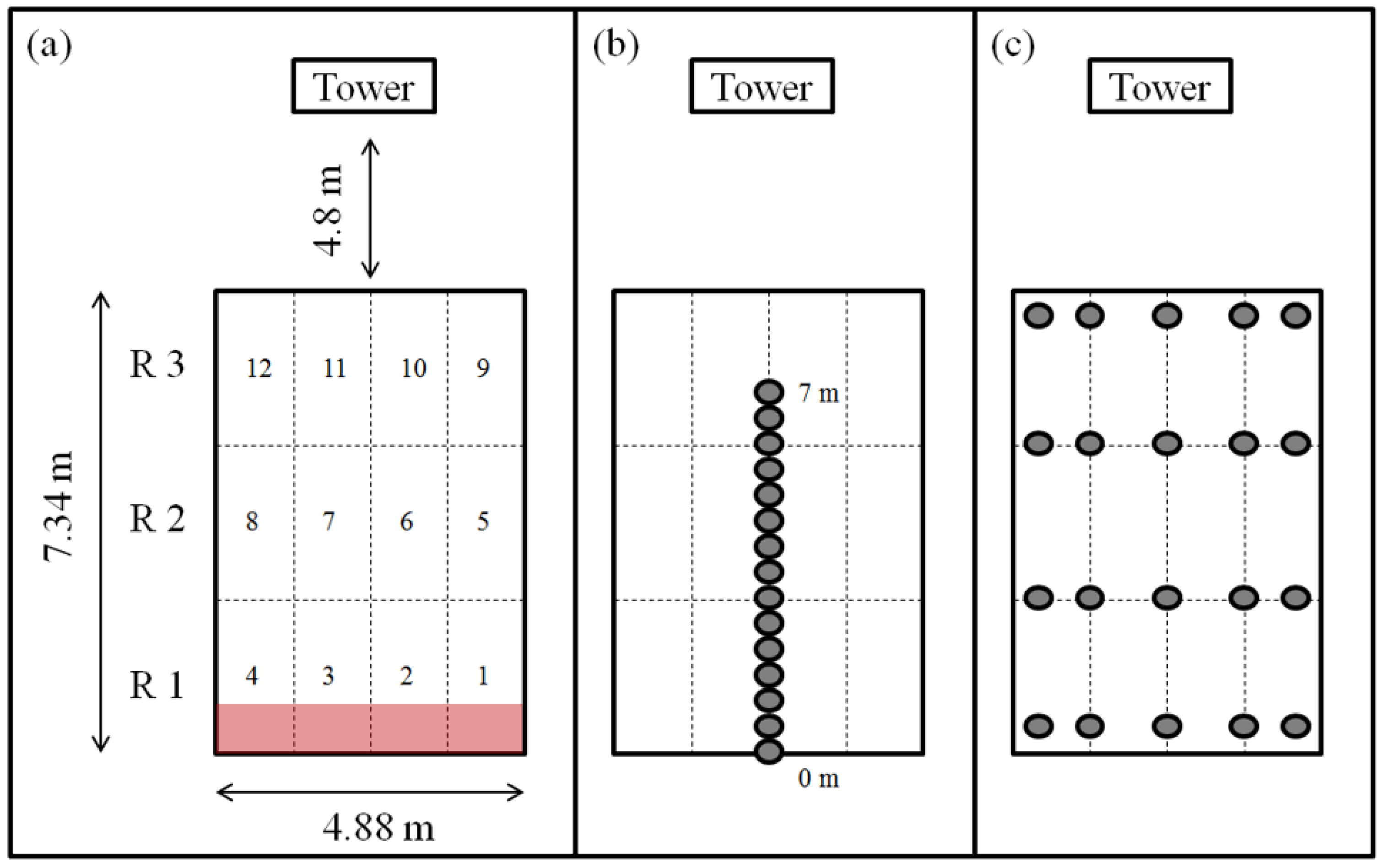
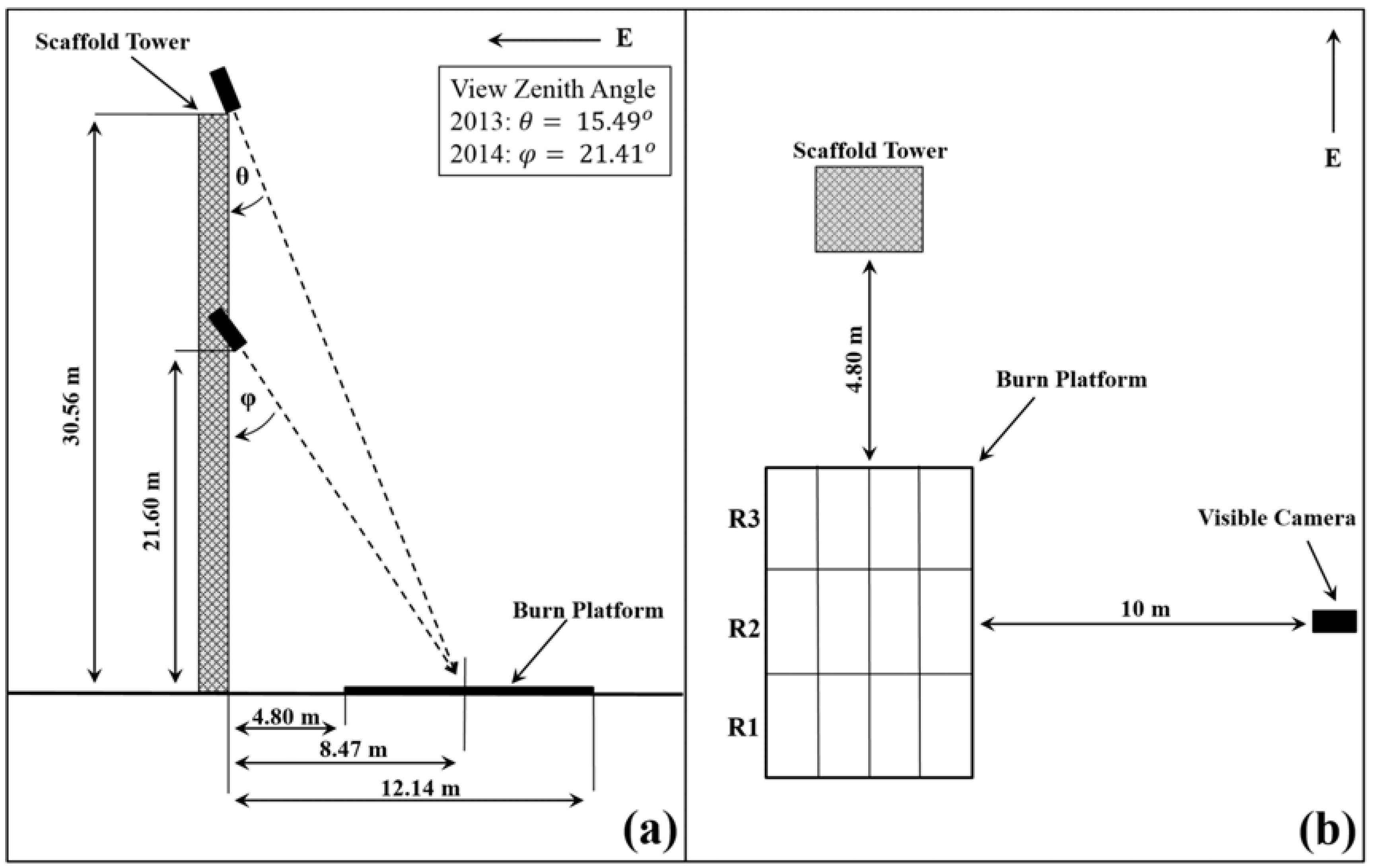
2.1. Experimental Design and Protocol
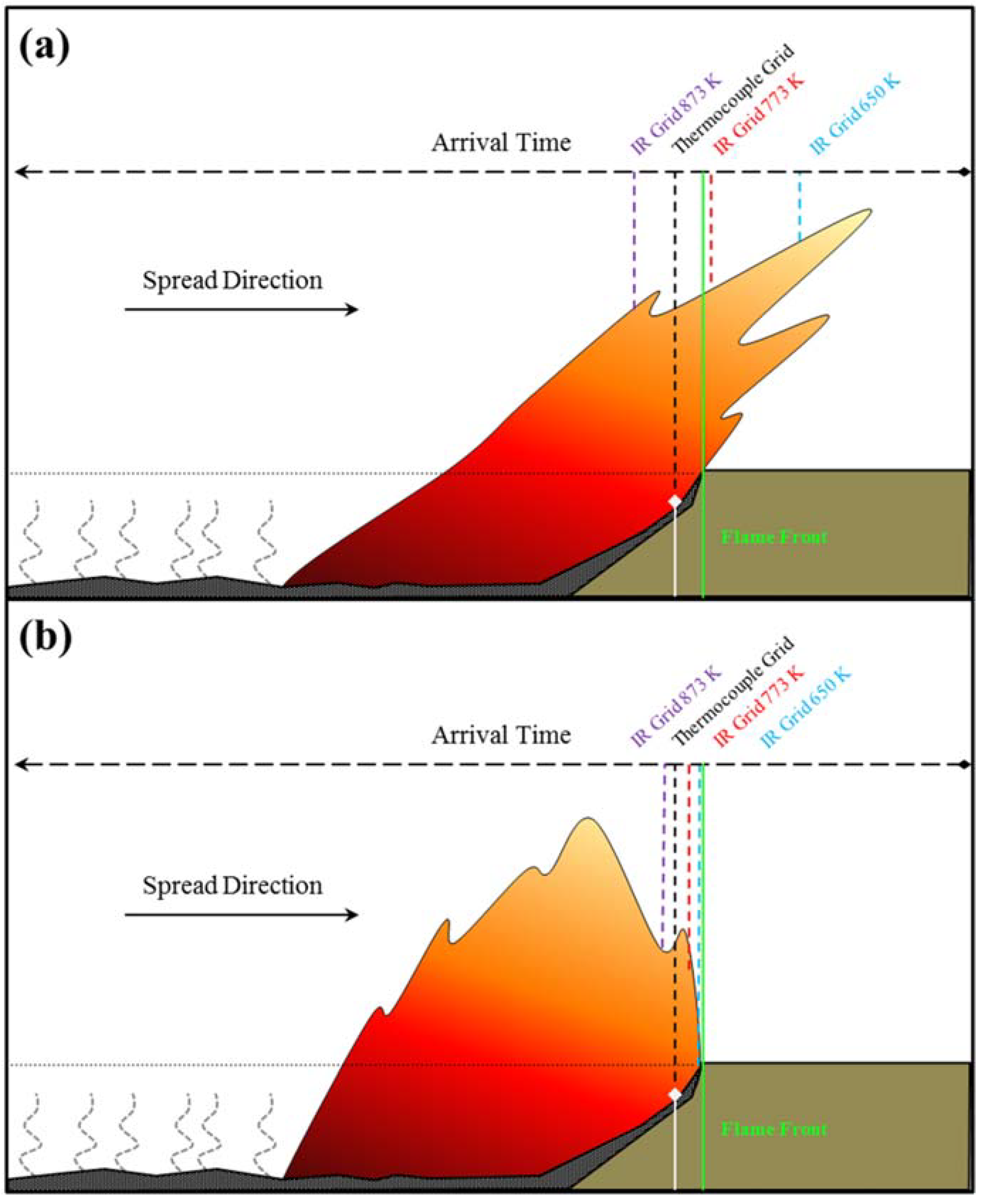
2.2. Methods of Calculating Rate of Spread
2.2.1. Visible Side and Visible Nadir Methods
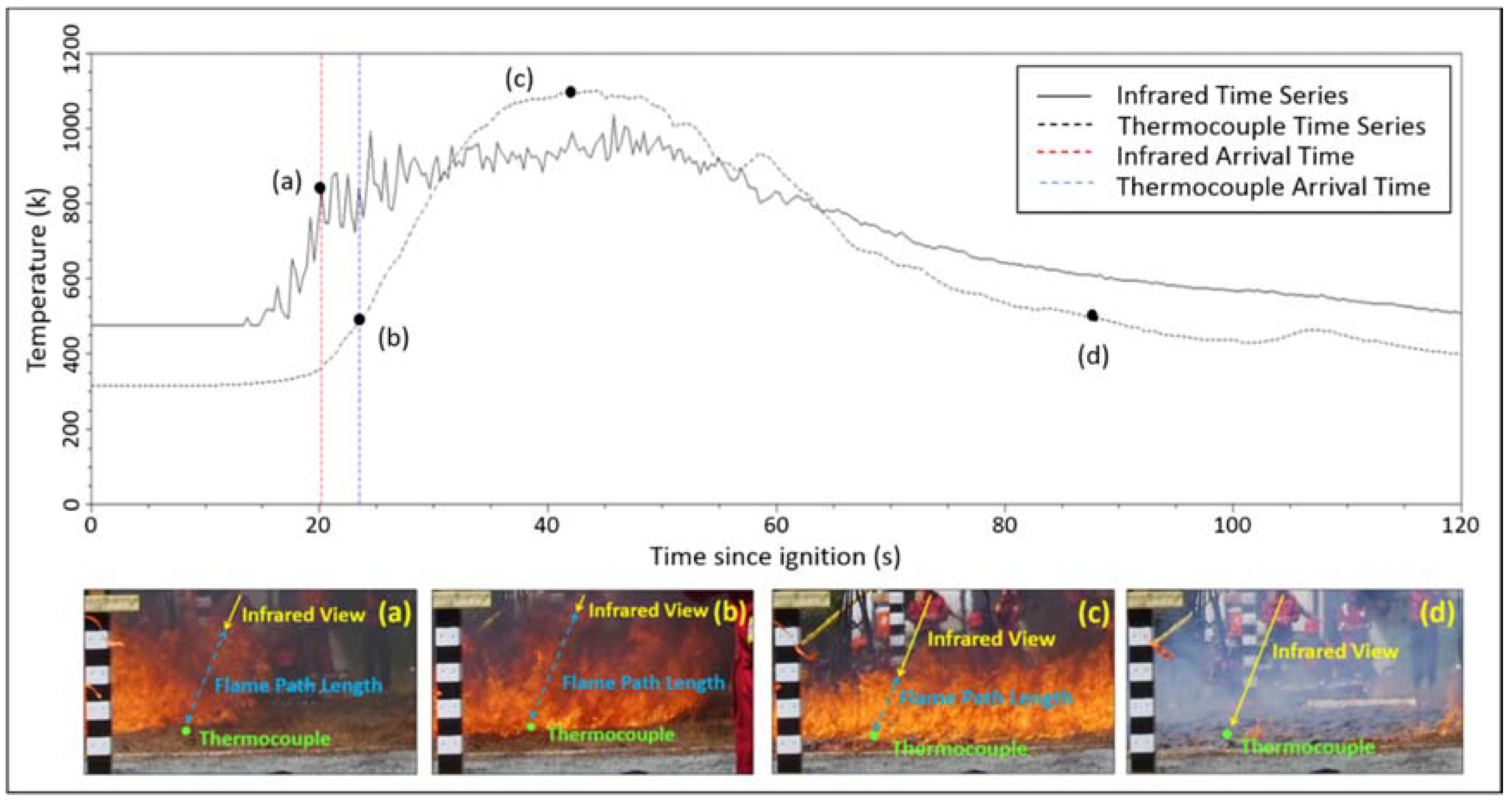
2.2.2. Thermocouple Linear Array
2.2.3. Thermocouple Grid Array (Standard Method)
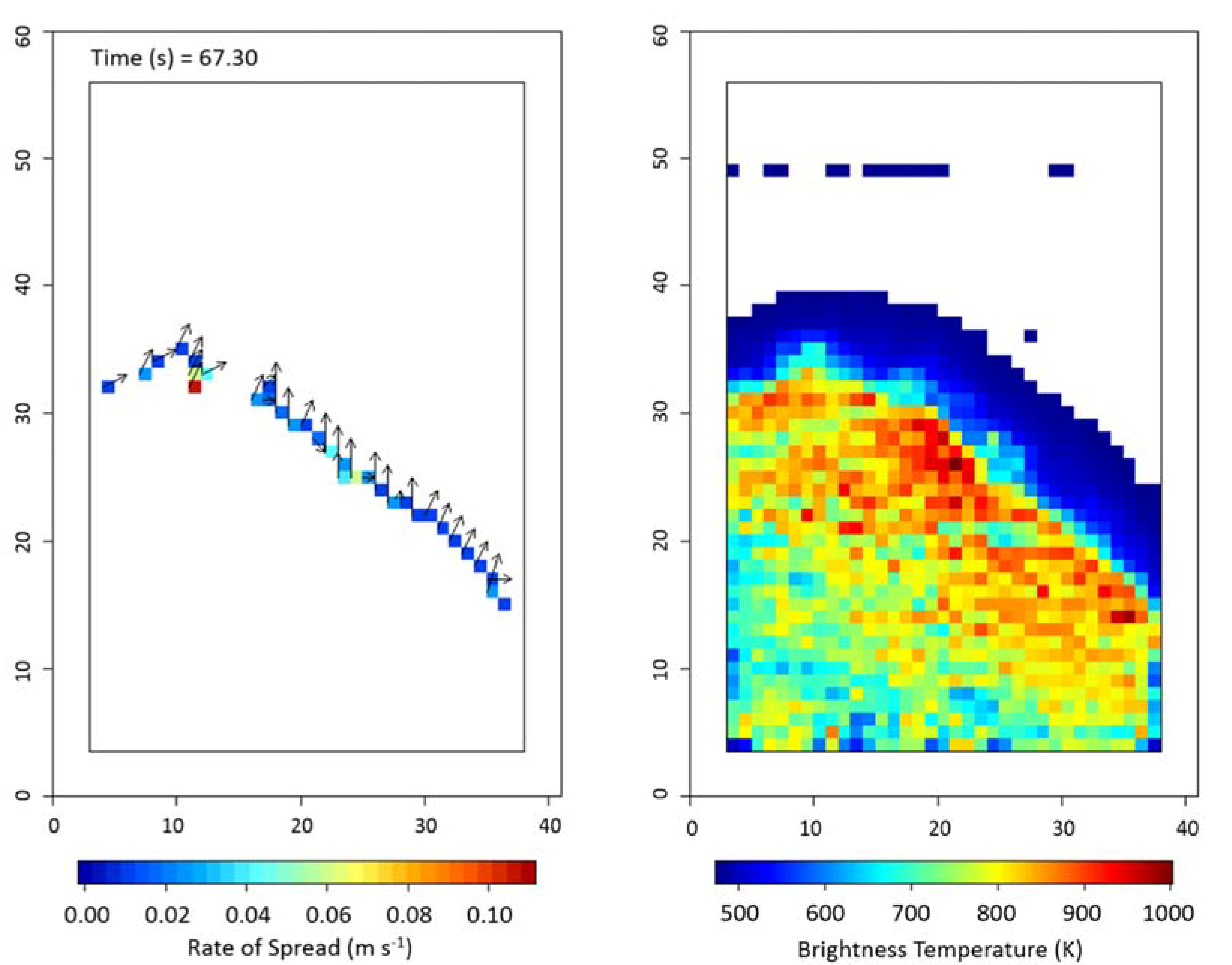
2.2.4. Infrared Grid Array
2.2.5. Infrared Paugam et al. 2013 Based Methods
2.2.6. Infrared Triangular Method
2.3. Analysis
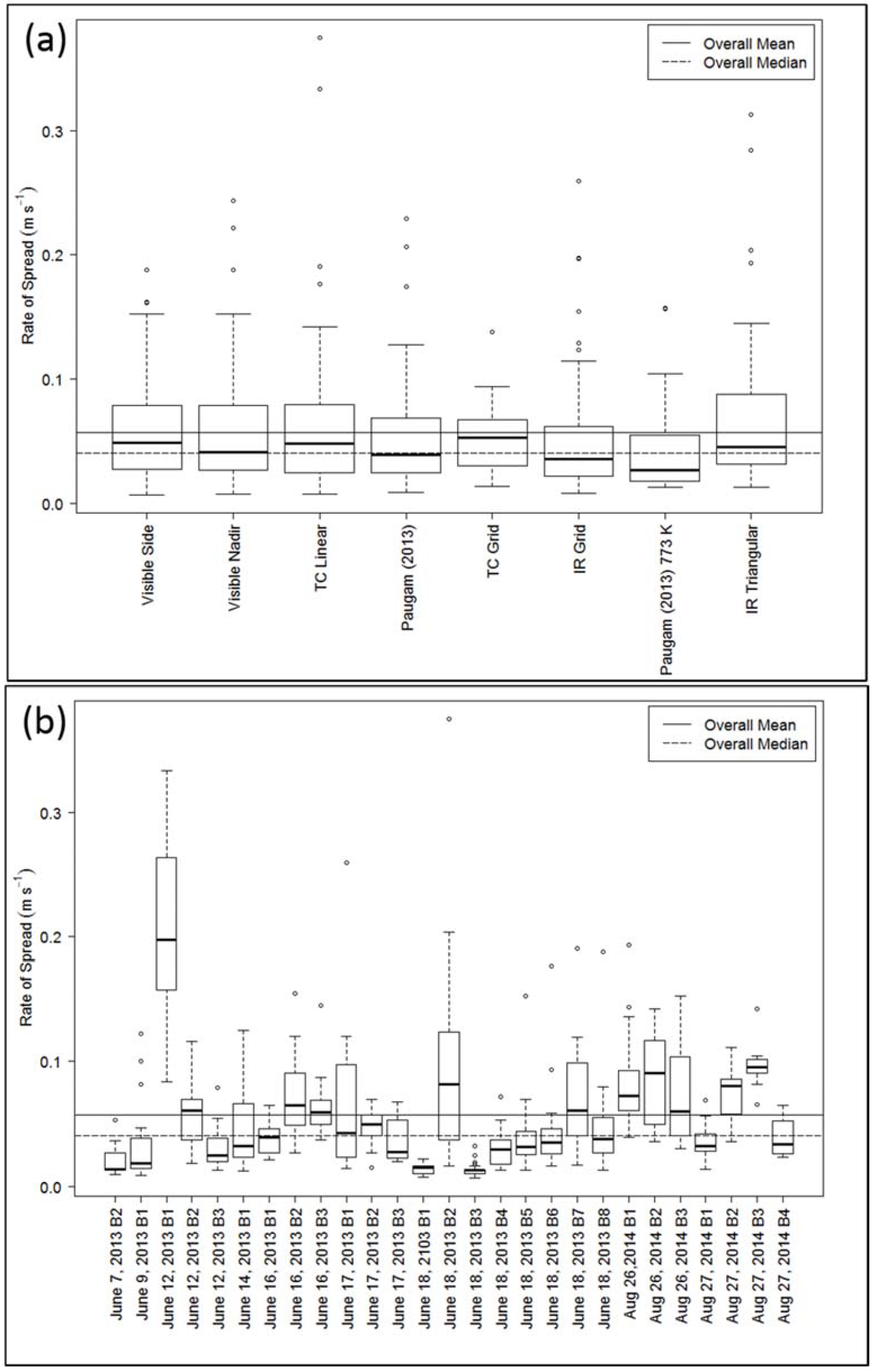
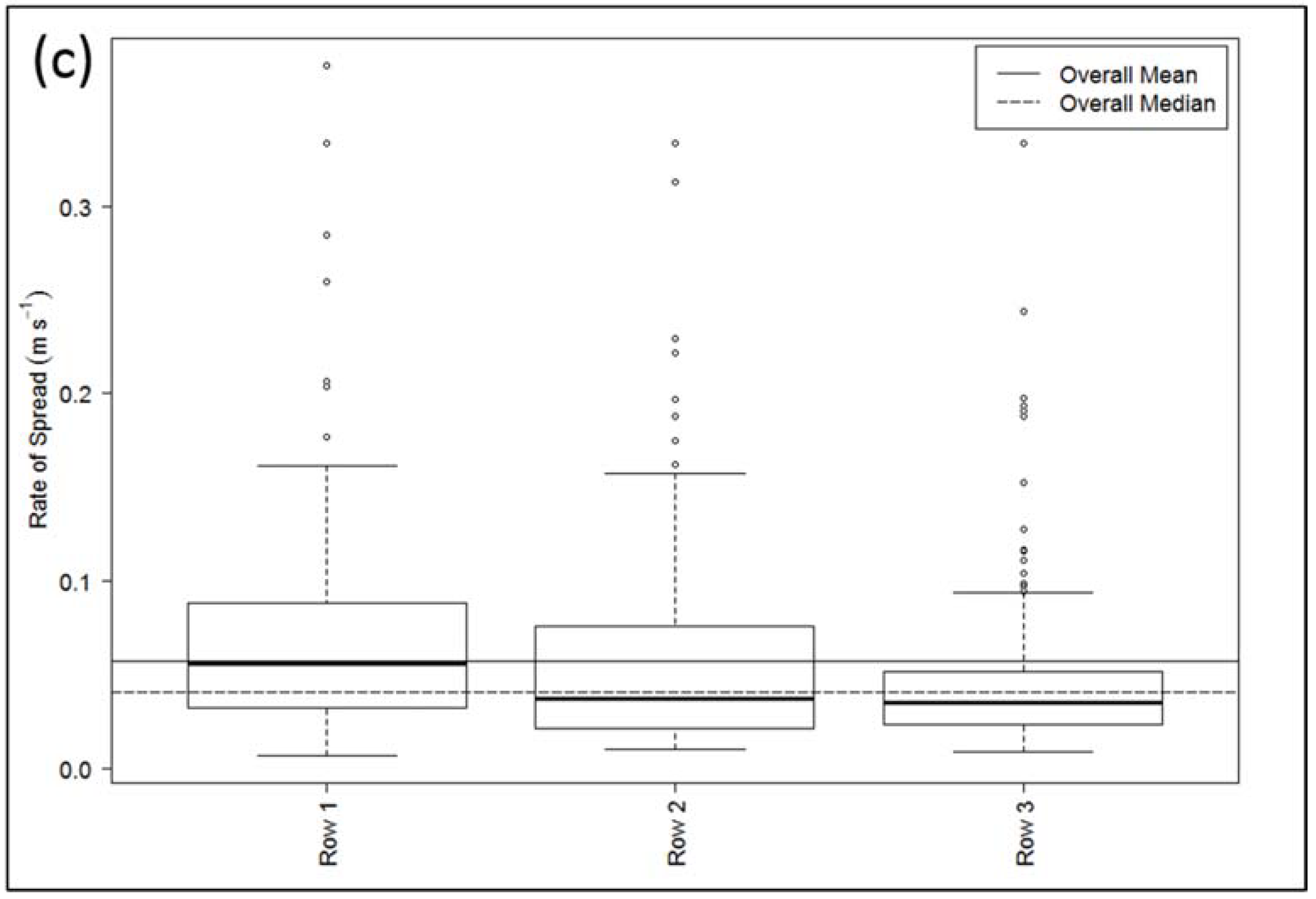
3. Results
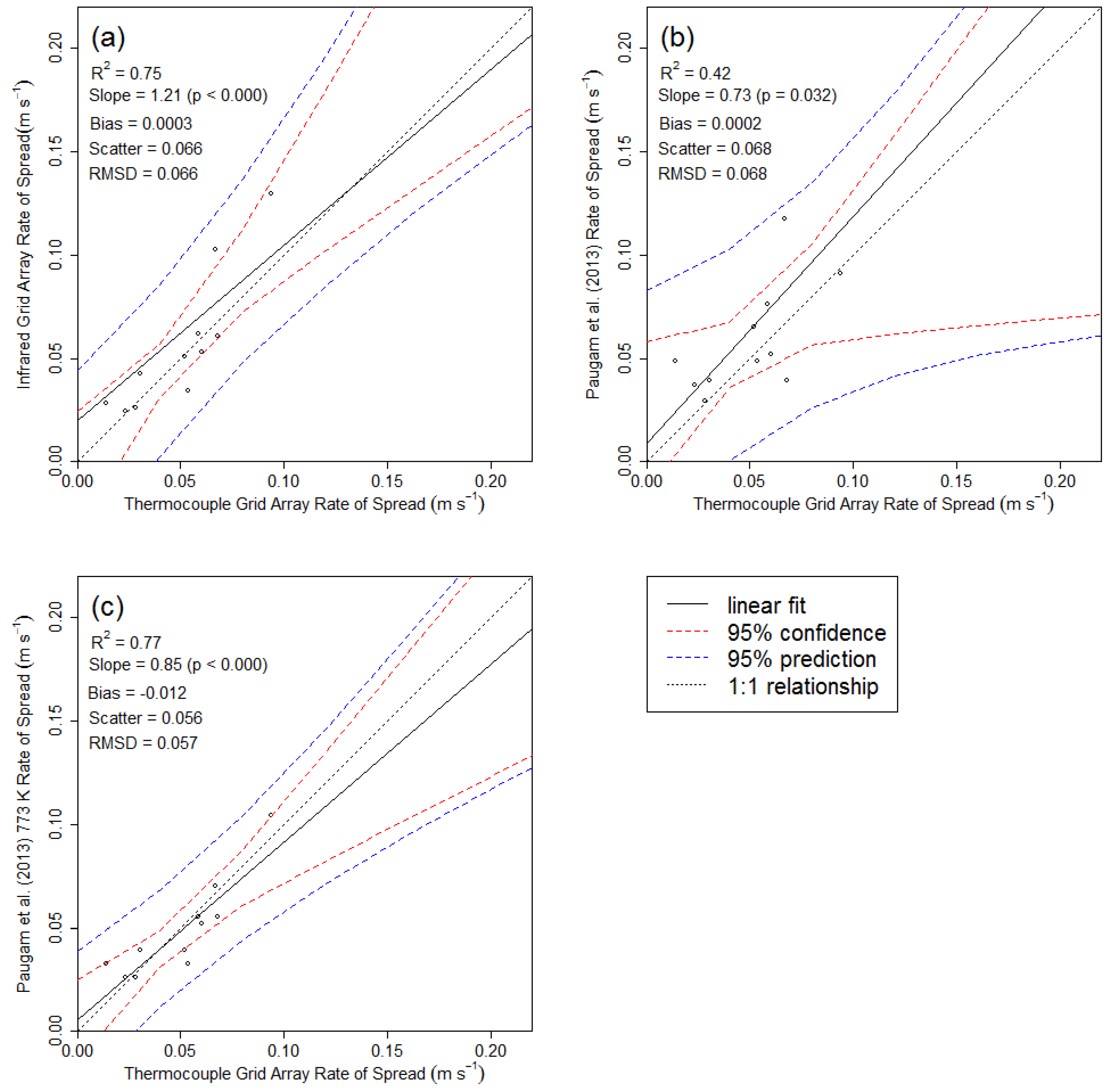
3.1. Comparison of Methods to One Another
3.2. Comparison of Measurements to Accepted Standard
4. Discussion and Conclusions
Supplementary Materials
Author Contributions
Acknowledgments
Conflicts of Interest
References
- Butler, B.; Cohen, J. Firefighter safety zones: A theoretical model based on radiative heating. Int. J. Wildland Fire 1998, 8, 73–77. [Google Scholar] [CrossRef]
- Alexander, M.E. Calculating and interpreting forest fire intensities. Can. J. Bot. 1982, 60, 349–357. [Google Scholar] [CrossRef]
- Byram, G.M. Forest fire behavior. In Forest Fire: Control and Use; Davis, K.P., Ed.; McGraw-Hill: New York, NY, USA, 1959; pp. 90–123. [Google Scholar]
- Van Wagner, C.E. Describing forest fires—Old ways and new. For. Chron. 1965, 41, 301–305. [Google Scholar] [CrossRef]
- Johnston, P.; Kelso, J.; Milne, G.J. Efficient simulation of wildfire spread on an irregular grid. Int. J. Wildland Fire 2008, 17, 614–627. [Google Scholar] [CrossRef]
- Cruz, M.G. Monte carlo-based ensemble method for prediction of grassland fire spread. Int. J. Wildland Fire 2010, 19, 521–530. [Google Scholar] [CrossRef]
- Andrews, P.L.; Cruz, M.G.; Rothermel, R.C. Examination of the wind speed limit function in the rothermel surface fire spread model. Int. J. Wildland Fire 2013, 22, 959–969. [Google Scholar] [CrossRef]
- Paugam, R.; Wooster, M.J.; Roberts, G. Use of handheld thermal imager data for airborne mapping of fire radiative power and energy and flame front rate of spread. IEEE Trans. Geosci. Remote Sens. 2013, 51, 1–15. [Google Scholar] [CrossRef]
- McArthur, A.G. Fire Behaviour in Eucalypt Forests; Forestry and Timber Bureau: Canberra, Australia, 1967. [Google Scholar]
- Forestry Canada Fire Danger Group. Development and Structure of the Canadian Forest Fire Behavior Prediction System; Information Report St-X-3; Forestry Canada, Ed.; Forestry Canada, Science and Sustainable Development Directorate: Ottawa, ON, Canada, 1992. [Google Scholar]
- Rothermel, R.C. A Mathematical Model for Predicting Fire Spread in Wildland Fuels; Res. Pap. Int-115; Department of Agriculture, Intermountain Forest and Range Experiment Station: Ogden, UT, USA, 1972; p. 40. [Google Scholar]
- Butler, B.W. Wildland firefighter safety zones: A review of past science and summary of future needs. Int. J. Wildland Fire 2014, 23, 295–308. [Google Scholar] [CrossRef]
- Putnam, T.; Butler, B.W. Evaluating fire shelter performance in experimental crown fires. Can. J. For. Res. 2004, 34, 1600–1615. [Google Scholar] [CrossRef]
- Sullivan, A.L.; Knight, I.K.; Cheney, N.P. Predicting the radiant heat flux from burning logs in a forest following a fire. Aust. For. 2002, 65, 59–67. [Google Scholar] [CrossRef]
- Zárate, L.; Arnaldos, J.; Casal, J. Establishing safety distances for wildland fires. Fire Saf. J. 2008, 43, 565–575. [Google Scholar] [CrossRef]
- Fryer, G.K.; Dennison, P.E.; Cova, T.J. Wildland firefighter entrapment avoidance: Modelling evacuation triggers. Int. J. Wildland Fire 2013, 22, 883–893. [Google Scholar] [CrossRef]
- Alexander, M.E.; Cole, F.V. Predicting and Interpreting Fire Intensities in Alaskan Black Spruce Forests Using the Canadian System of Fire Danger Rating; Society of American Foresters/Canadian Institute of Forestry Convention 1994, Bethesda, Maryland, 1995; Society of American Foresters: Bethesda, MA, USA, 1994; pp. 185–192. [Google Scholar]
- De Groot, W.J. Modeling fire effects: Integrating fire behavior and fire ecology. In Proceedings of the 6th International Conference on Forest Fire Research, Coimbra, Portugal, 15–18 November 2010. [Google Scholar]
- De Groot, W.J.; Bothwell, P.M.; Taylor, S.W.; Wotton, B.M.; Stocks, B.J.; Alexander, M.E. Jack pine regeneration and crown fires. Can. J. For. Res. 2004, 34, 1634–1641. [Google Scholar] [CrossRef]
- De Groot, W.J.; McRae, D.J.; Ivanova, G.A. Modeling fire behaviour, fuel consumption and wildlandfire carbon emissions in Canadian and Russian boreal forests. In Proceedings of the 3rd International Fire Ecology and Management Congress, San Diego, TX, USA, 13–17 November 2006. [Google Scholar]
- Smith, A.M.S.; Talhelm, A.F.; Johnson, D.M.; Sparks, A.M.; Kolden, C.A.; Yedinak, K.M.; Apostol, K.G.; Tinkham, W.T.; Abatzoglou, J.T.; Lutz, J.A.; et al. Effects of fire radiative energy density dose on pinus contorta and larix occidentalis seedling physiology and mortality. Int. J. Wildland Fire 2017, 26, 82–94. [Google Scholar] [CrossRef]
- Albini, F.A. A model for fire spread in wildland fuels by-radiation. Combust. Sci. Technol. 1985, 42, 229–258. [Google Scholar] [CrossRef]
- Rivera, J.d.D.; Davies, G.M.; Jahn, W. Flammability and the heat of combustion of natural fuels: A review. Combust. Sci. Technol. 2012, 184, 224–242. [Google Scholar] [CrossRef]
- Simard, A.J.; Deacon, A.G.; Adams, K.B. Nondirectional sampling of wildland fire spread. Fire Technol. 1982, 18, 221–228. [Google Scholar] [CrossRef]
- Taylor, S.W.; Pike, R.G.; Alexander, M.E. Field Guide to the Canadian Forest Fire Behaviour Prediction (fbp) System; Canadian Forest Service, Ed.; Northern Forestry Centre: Edmonton, AB, Canada, 1997. [Google Scholar]
- Simard, A.J.; Eenigenburg, J.E.; Adams, K.B.; Nissen, J.R.L.; Deacon, A.G. A general procedure for sampling and analyzing wildland fire spread. For. Sci. 1984, 30, 51–64. [Google Scholar]
- Alexander, M.E.; Lanoville, R.A. Wildfires as a source of fire behavior data: A case study from Northwest Territories, Canada. In Proceedings of the Ninth Conference on Fire and Forest Meteorology, San Diego, CA, USA, 21–24 April 1987. [Google Scholar]
- Alexander, M.E.; Lawson, B.D.; Stocks, B.J.; van Wagner, C.E. User Guide to the Canadian Forest Fire Behaviour Prediction System: Rate of Spread Relationships; (Interim Edition); Environment Canada, Canadian Forestry Service: Northern Forest Research Centre: Edmonton, AB, Canada, 1984. [Google Scholar]
- Wotton, B.; Martin, T. Temperature Variation in Vertical Flames from a Surface Fire. In Proceedings of the III International Conference on Forest Fire Research/14th Conference on Forest and Fire Meteorology, Luso, Portugal, 16–20 November 1998; pp. 533–545. [Google Scholar]
- Mendes-Lopes, J.; Ventura, J.; Amaral, J. Flame characteristics, temperature-time curves, and rate of spread in fires propagating in a bed of pinus pinaster needles. Int. J. Wildland Fire 2003, 12, 67–84. [Google Scholar] [CrossRef]
- Dupuy, J.; Maréchal, J.; Portier, D.; Valette, J.-C. The effects of slope and fuel bed width on laboratory fire behaviour. Int. J. Wildland Fire 2011, 20, 272–288. [Google Scholar] [CrossRef]
- Butler, B.; Teske, C.; Jimenez, D.; O’Brien, J.; Sopko, P.; Wold, C.; Vosburgh, M.; Hornsby, B.; Loudermilk, E. Observations of energy transport and rate of spreads from low-intensity fires in longleaf pine habitat—RxCADRE 2012. Int. J. Wildland Fire 2016, 25, 76–89. [Google Scholar] [CrossRef]
- Taylor, S.W.; Wotton, B.M.; Alexander, M.E.; Dalrymple, G.N. Variation in wind and crown fire behaviour in a northern jack pine-black spruce forest. Can. J. For. Res. 2004, 34, 1561–1576. [Google Scholar] [CrossRef]
- Wotton, B.; Gould, J.; McCaw, W.; Cheney, N.; Taylor, S. Flame temperature and residence time of fires in dry eucalypt forest. Int. J. Wildland Fire 2012, 21, 270–281. [Google Scholar] [CrossRef]
- McRae, D.J.; Jin, J.Z.; Conard, S.G.; Sukhinin, A.I.; Ivanova, G.A.; Blake, T.W. Infrared characterization of fine-scale variability in behavior of boreal forest fires. Can. J. For. Res. 2005, 35, 2194–2206. [Google Scholar] [CrossRef]
- Stocks, B.J. Fire behaviour in immature jack pine. Can. J. For. Res. 1987, 17, 80–86. [Google Scholar] [CrossRef]
- Stocks, B.J. Fire behaviour in mature jack pine. Can. J. For. Res. 1989, 19, 783–790. [Google Scholar] [CrossRef]
- Pastor, E.; Àgueda, A.; Andrade-Cetto, J.; Muñoz, M.; Pérez, Y.; Planas, E. Computing the rate of spread of linear flame fronts by thermal image processing. Fire Saf. J. 2006, 41, 569–579. [Google Scholar] [CrossRef] [Green Version]
- Stephens, S.L.; Weise, D.R.; Fry, D.L.; Keiffer, R.J.; Dawson, J.; Koo, E.; Potts, J.B.; Pagni, P.J. Measuring the rate of spread of chaparral prescribed fires in Northern California. J. Assoc. Fire Ecol. 2008, 4, 74–86. [Google Scholar] [CrossRef]
- Johnston, J.M.; Wooster, M.J.; Paugam, R.; Wang, X.; Lynham, T.J.; Johnston, L.M. Direct estimation of byram’s fire intensity from infrared remote sensing imagery. Int. J. Wildland Fire 2017, 26, 668–684. [Google Scholar] [CrossRef]
- Exelis Visual Information Solutions. IDL Basics; Exelis Visual Information Solutions: Boulder, CO, USA, 2010. [Google Scholar]
- Burrows, N.D. Flame residence time and rates of weight loss of eucalypt forest fuel particles. Int. J. Wildland Fire 2001, 10, 137–143. [Google Scholar] [CrossRef]
- Johnston, J.M.; Wooster, M.J.; Lynham, T.J. Experimental confirmation of the MWIR and LWIR greybody assumption for vegetation fire flame emissivity. Int. J. Wildland Fire 2014, 23, 463–479. [Google Scholar] [CrossRef]
- R Core Team. R: A Language and Environment for Statistical Computing. Available online: http://www.r-project.org/ (accessed on 7 May 2018).
- Bates, D.; Maechler, M.; Bolker, B.; Walker, S. Fitting linear mixed-effects models using lme4. J. Stat. Softw. 2015, 67, 1–48. [Google Scholar] [CrossRef]
- Kuznetsova, A.; Brockhoff, P.B.; Christensen, R.H.B. Lmertest: Tests in Linear Mixed Effects Models. Available online: https://cran.r-project.org/web/packages/lmerTest/index.html (accessed on 7 May 2018).
- Legg, C.; Davies, M.; Kitchen, K.; Marno, P. A Fire Danger Rating System for Vegetation Fires in the Uk: The Firebeaters Project Phase 1 Final Report; The University of Edinburgh and The Met Office: Edinburgh, UK, 2007. [Google Scholar]
- Wooster, M.J.; Roberts, G.; Smith, A.M.S.; Johnston, J.; Freeborn, P.; Amici, S.; Hudak, A.T. Thermal remote sensing of active vegetation fires and biomass burning events. In Thermal Infrared Remote Sensing; Kuenzer, C., Dech, S., Eds.; Springer: Dordrecht, The Netherlands, 2013; Volume 17, pp. 347–390. [Google Scholar]
- National Infrared Operations. Available online: https://fsapps.nwcg.gov/nirops/pages/about (accessed on 6 April 2018).


| Method Reference | Method Description | Data Source | Fire Arrival Threshold | Direction of Spread | Field Deployment | Data Processing | Number of Fires with Data Available |
|---|---|---|---|---|---|---|---|
| Visible Side | Fire spread recorded with VIS camera at ground level. Visual analysis to determine time lapse between fixed locations. | VIS Imagery | Visual | NA | Ground observations | Manual interpretation, minimal calculation | 27 |
| Visible Nadir | Fire spread recorded with VIS camera on tower at near nadir position. Visual analysis to determine time lapse between fixed locations. | VIS Imagery | Visual | NA | Aircraft observation | Manual interpretation, minimal calculation | 27 |
| Thermocouple Linear Array | Linear array of 15 thermocouples at 0.5 m intervals extending perpendicular to the ignition line along the center of the burn platform. Fire arrival determined at each position via temperature threshold. | Thermocouples | 573 K | NA | Ground instrumentation | Partially automated, minimal calculation | 27 |
| Thermocouple Grid Array | Grid of 20 thermocouples positioned uniformly throughout the burn platform. Fire arrival determined at each position via temperature threshold. Arrival times used in Simard et al. (1984) method, averages for each panel of burn pad reported. | Thermocouples | 573 K | Geometrically calculated | Ground instrumentation | Partially automated | 7 |
| Infrared Grid Array | Geo-referenced nadir positioned IR brightness temperature time series used to replace the 20 thermocouples in the thermocouple grid method, otherwise method remains unchanged. | IR Imagery | 773 K | Geometrically calculated | Airborne IR (requires geo-referencing) | Fully automated, computationally intensive | 24 |
| Paugam et al. (2013) | Direct application of the method of Paugam et al. (2013). Bonfire ground control points are not used due to fixed IR camera position on top of nearby tower. Flame front arrival is determined via brightness temperature threshold and RoS computed normal to the flame at each pixel. | IR Imagery | 650 K | Normal at each pixel | Airborne IR (requires geo-referencing) | Fully automated, computationally intensive | 24 |
| Paugam et al. (2013) 773 K | Variant of the IR Paugam et al. (2013) methodology in which the fire arrival temperature threshold is raised to 773 K. | IR Imagery | 773 K | Normal at each pixel | Airborne IR (requires geo-referencing) | Fully automated, computationally intensive | 24 |
| Infrared Triangular Method | Variant of the method described in McRae et al. (2005). In this method IR imagery is geo-referenced, and calculations are performed directly on raster data. Fire arrival times from adjacent perimeter pixels are used in the Simard et al. (1984) method and reported by pixel. | IR Imagery | 773 K | Geometrically calculated by pixel cluster | Airborne IR (requires geo-referencing) | Fully automated, computationally intensive | 24 |
| Fixed Effect (RoS Method) | DF | T | p |
|---|---|---|---|
| Visible side | 425.2 | 1.176 | 0.240 |
| Visible nadir | 425.2 | 1.340 | 0.181 |
| Thermocouple Linear Array | 426.1 | 2.591 | 0.010 * |
| Infrared Grid Array | 427.1 | 1.211 | 0.227 |
| Paugam et al. (2013) | 427.0 | 0.749 | 0.454 |
| Paugam et al. (2013) 773 K | 426.9 | −0.500 | 0.618 |
| Infrared Triangular Method | 426.9 | 2.352 | 0.019 * |
| RoS Method | DF | Critical T | Slope | SE | T | p |
|---|---|---|---|---|---|---|
| Infrared Grid Array | 8 | 2.306 | 1.123 | 0.234 | −0.526 | 0.613 |
| Paugam et al. (2013) | 8 | 2.306 | 0.733 | 0.289 | 0.924 | 0.383 |
| Paugam et al. (2013) 773 K | 8 | 2.306 | 0.858 | 0.158 | 0.899 | 0.395 |
| Intensity Class | Fire Intensity (kW m−1) | Rate of Spread (m s−1) | Description |
|---|---|---|---|
| 1 | <10 | <0.001 | Smoldering/creeping |
| 2 | 10–500 | 0.001–0.032 | Surface fire with open flame, flame heights ~ 1.0 m |
| 3 | 500–2000 | 0.033–0.12 | Vigorous surface fire with short-range spotting |
| 4 | 2000–4000 | 0.12–0.25 | Intermittent crown fire |
| 5 | 4000–10,000 | 0.25–0.64 | Continuous crown fire, major suppression campaign |
| 6 | >10,000 | >0.64 | Continuous crown fire with extreme fire behavior, limited suppression potential |
© 2018 by the authors. Licensee MDPI, Basel, Switzerland. This article is an open access article distributed under the terms and conditions of the Creative Commons Attribution (CC BY) license (http://creativecommons.org/licenses/by/4.0/).
Share and Cite
Johnston, J.M.; Wheatley, M.J.; Wooster, M.J.; Paugam, R.; Davies, G.M.; DeBoer, K.A. Flame-Front Rate of Spread Estimates for Moderate Scale Experimental Fires Are Strongly Influenced by Measurement Approach. Fire 2018, 1, 16. https://doi.org/10.3390/fire1010016
Johnston JM, Wheatley MJ, Wooster MJ, Paugam R, Davies GM, DeBoer KA. Flame-Front Rate of Spread Estimates for Moderate Scale Experimental Fires Are Strongly Influenced by Measurement Approach. Fire. 2018; 1(1):16. https://doi.org/10.3390/fire1010016
Chicago/Turabian StyleJohnston, Joshua M., Melanie J. Wheatley, Martin J. Wooster, Ronan Paugam, G. Matt Davies, and Kaitlin A. DeBoer. 2018. "Flame-Front Rate of Spread Estimates for Moderate Scale Experimental Fires Are Strongly Influenced by Measurement Approach" Fire 1, no. 1: 16. https://doi.org/10.3390/fire1010016