Some Requirements for Simulating Wildland Fire Behavior Using Insight from Coupled Weather—Wildland Fire Models


National Center for Atmospheric Research, P.O. Box 3000, Boulder, CO 80301, USA
Fire 2018, 1(1), 6; https://doi.org/10.3390/fire1010006
Submission received: 29 December 2017
/
Revised: 2 February 2018
/
Accepted: 6 February 2018
/
Published: 9 February 2018
Abstract
:A newer generation of models that interactively couple the atmosphere with fire behavior have shown an increased potential to understand and predict complex, rapidly changing fire behavior. This is possible if they capture intricate, time-varying microscale airflows in mountainous terrain and fire-atmosphere feedbacks. However, this benefit is counterbalanced by additional limitations and requirements, many arising from the atmospheric model upon which they are built. The degree to which their potential is realized depends on how coupled models are built, configured, and applied. Because these are freely available to users with widely ranging backgrounds, I present some limitations and requirements that must be understood and addressed to achieve meaningful fire behavior simulation results. These include how numerical weather prediction models are formulated for specific scales, their solution methods and numerical approximations, optimal model configurations for common scenarios, and how these factors impact reproduction of fire events and phenomena. I discuss methods used to adjust inadequate outcomes and advise on critical interpretation of fire modeling results, such as where errors from model limitations may be misinterpreted as natural unpredictability. I discuss impacts on other weather model-based applications that affect understanding of fire behavior and effects.
1. Introduction
Wildland fire behavior models have been developed and applied since the early 1970s to understand observed incidents, anticipate fire growth, and test the effect of varying environmental conditions on fire behavior. Early models were primarily diagnostic kinematic formulae or empirical relationships based on theory, laboratory fire beds, or small-scale prescribed fire experiments (e.g., [1,2]). Subsequent tools implemented these formulae in two-dimensions along with a constraint that the fire overall [3,4] or local heading regions [5] maintain a particular shape, often elliptical. In these, wind may remain steady state or, as in some current operational tools (e.g., [6,7]), estimate time-varying winds. These models explained some spatial variability in fire growth across the landscape and when connected to additional algorithms—consumption, fire effects, and plume models—could also be used to estimate fire effects and emissions.
A newer class of models—coupled atmosphere-fire models—appeared in the 1990s (e.g., [8,9,10]). Coupled models integrated the prior fire behavior models or modules parameterizing wildland fuel combustion with some type of computational fluid dynamics (CFD) model. In contrast to prior tools, coupled models are prognostic (i.e., predict the time rate of change of atmospheric variables), calculate how fire behavior changes in response over time, and are dynamic (i.e., represent the exchange of forces between a fire and the surrounding atmosphere). Coupled systems simulate evolving atmospheric conditions which direct fire behavior, while heat and other combustion products from the fire are released into and alter the atmospheric state, feedbacks subsequently referred to as “fire-atmosphere interactions”. This two-way physical coupling shapes the winds near the fire and, even without explicit modeling of combustion or flames, allows some natural fire behavior, such as the commonly observed elliptical fire shape, to emerge. Coupling allows the separate effects of fuel, terrain, and wind to multiply through dynamic interactions. Coupled models thus have the potential to extend our ability to understand and anticipate more complex, rapidly changing aspects of fire behavior.
However, this higher level of complexity is accompanied by other limitations and requirements, often of the atmospheric model upon which they are built. In addition, the degree to which this potential is realized depends on how coupled models are built, configured, and applied, and crucial details that have been underemphasized or overlooked in scientific literature to date. Here, I present some limitations and requirements that must be met to achieve meaningful fire behavior simulation results to advise potential users on model selection, development, and use and to guide interpretation of model outcomes. It may also inform readers without detailed technical knowledge who appreciate the phenomenon’s complexity and wish to learn more about the methodology. This discussion provides perspective on perceptions that fire behavior now exceeds fire models or the persistent notion that fire behavior is unpredictable.
2. Background
Wildland fire perimeters evolve in peculiar shapes but the reasons for a specific surge of growth are often not apparent or explicable from available environmental or land surface data. Wildland fires may bifurcate into multiple heading regions, flank runs, or merge. They may generate a wide range of dynamic, transient phenomena including fire whirls, horizontal roll vortices, collapsing plumes, flaming fingers, wind shifts, blow ups, pyrocumuli, and wind speeds that are among the extremes of atmospheric phenomena. Misanticipating fire behavior and rapidly changing conditions can lead to fire fighter burnovers [11]. Thus, scientific modeling studies have been developed to understand fire behavior and operational forecasting applications to warn of dangerous conditions.
Coupled atmosphere-fire models have the potential to recreate and perhaps anticipate many fire phenomena. Previous work has already demonstrated the unfolding of a wildfire including timing of important transitions and distinctive shape, and emergence of transient fire phenomena including wind shifts [12], fire whirls [13,14,15,16], and horizontal roll vortices [17]. These advances were attributed to resolving the intricate, time-varying airflow in mountainous terrain at spatial resolutions of about one hundred meters and including fire-atmosphere feedbacks exemplified by plume dominated fires. Other studies have been used to test disturbance effects [18] and, with limited success, to simulate prescribed fires [19]. Several coupled models are distributed by developers or through internet download and thus reach a broad user community beyond those with experience in atmospheric modeling or fire behavior. This has created a need for better understanding of the possibilities and requirements that has not yet appeared.
Warner [20] discussed a concurrent change underlying the evolution in fire modeling systems which is the increasing and broadening use of atmospheric models. In the 1980s, atmospheric models were primarily developed and used by scientists with atmospheric science degrees. Since then, the number of model users and the variability in their scientific and technical training has increased rapidly. Factors responsible for this increase include the wide availability of community atmospheric models, support and training for their use, the declining cost and increasing availability of computational resources, increasing model skill, development of add-on modules extending weather model use to other application areas, and the growing use of atmospheric models by specialists from other scientific areas. He discussed how factors related to the broadening user base—lack of specific numerical weather prediction or even atmospheric science courses—could lead to model use that strayed from best practices as users lacked experience from which to recognize when a simulation looked faulty or identify the cause, whether due to configuration choices or model design. He cautioned against using a model as a black box and advised that it is important to have a physical understanding of processes, phenomena, and what is required to produce and represent them, and to spend time learning to understand time-varying atmospheric airflow. Noting that models are ‘complex and imperfect tools and that their shortcomings should be understood well by every model user’ ([20], p. 1602), he discussed best practices for atmospheric model use. His recommendations apply here too, as atmospheric models serve as the basis for coupled weather-fire models and, due to the interdisciplinary nature of fire research, coupled model users come from disciplines outside atmospheric or even physical science including engineering, computer science, mathematics, and the life sciences (e.g., ecology and forest science).
3. Simulating Weather Well
CFD models solve a set of partial differential equations based on the Navier-Stokes equations of motion that describe the time-varying flow of viscous fluids such as air along with relationships based on the second law of thermodynamics, the ideal gas law, and conservation of mass (see [21,22]). Exact analytical solutions exist only for certain idealized problems thus, in practice, the equations are discretized on a gridded mesh of points and the state variables’ evolution is solved by calculating the variables’ time rate of change at each point. The rate of change depends on transport from nearby locations, dissipation, sources and sinks from physical processes, and, for velocity components, accelerations due to pressure gradients and buoyancy. Models iteratively advance these variables time step by time step.
One type of coupled model combines CFD models used to simulate airflows in fine grid spacing (~1 m) in small domains (under ~1 km3) with equations that parameterize the combustion of wildland fuels but omit extensions that would treat weather processes (e.g., High-Resolution Model for Strong Gradient Applications (HIGRAD)/FIRETEC [10] subsequently referred to as FIRETEC, and the Wildland Fire Dynamic Simulator (WFDS) [23,24]). Another type combines a different type of CFD model—a numerical weather prediction (NWP) model—with empirical or semi-empirical relationships describing fire behavior. NWP models are designed for simulations at grid spacing of tens of meters to tens of kilometers, depending on the focus and design, and employ additional prognostic equations for water species and precipitation variables, adaptations for flows in complex terrain, treatments for momentum, heat, and moisture exchanges with the earth’s surface, nested domains to refine grid spacing over several orders of magnitude, and lateral boundaries that are usually open to introduce time-changing atmospheric conditions. The differing level of detail in the parameterization of fire processes between the two types reflects the factor of 100 or more difference in grid spacing at which they operate. When used appropriately, there is little overlap in problems that both types of coupled atmosphere-fire modeling systems may consider, thus limiting comparisons.
Wildland fire behavior is complicated by the complex atmospheric flows that occur over mountainous terrain. Mountain meteorology, a specialty area within atmospheric science, has explored how factors such as atmospheric winds; thermodynamic effects from static stability, solar heating, and precipitate/condensate phase changes; and terrain structure and roughness produce specific airflow regimes and phenomena [25,26,27]. The three-dimensional, time-dependent nature of airflow regimes—characteristic flow patterns that occur when flow parameters such as terrain aspect ratio (i.e., elevation rise over horizontal distance), wind speed, atmospheric stability, and surface roughness each fall within a specific range—has been slow to integrate into fire behavior understanding due to its mathematical and physical complexity. In forested ecosystems, turbulent airflows above and within tree canopies [28] further modulate atmospheric structure.
The aforementioned set of fluid dynamics, thermodynamics, and conservation equations is the minimum set that can encompass the temporally and spatially varying variables that make up atmospheric fluid flow; no simpler set of equations can reliably suffice in all conditions and locations. However, terms within these equations may be neglected due to their relative unimportance at the scale of motion being simulated, such as vertical motion in large-scale NWP models or the Coriolis effect in fine-scale NWP models. Various airflow estimators [29,30] put forth within the wildland fire community assume additional terms within these equations or some equations themselves can be neglected, citing the need for reduced complexity, computational cost, or the need to compute in the field. Wind Ninja and Wind Wizard have been suggested as simpler tools than full weather models and are widely used within the fire community to estimate the spatial distribution of surface winds in complex terrain near fires. These neglect time dependence, thermodynamic heating/cooling, and vertical motion—however, these terms all make important contributions to air acceleration in complex terrain [27] and thus are important factors that shape the wind driving fires. For example, the airflow in the lee of Askervein hill, a flow used to test the diagnostic model in [30], has no steady state solution; instead, it is comprised of intermittent, recirculating eddies [31], a flow regime these steady-state models cannot capture. These tools’ output may appear more realistic than uniform wind fields previously used with kinematic tools such as FARSITE, showing simple effects such as acceleration over the top of a hill. In addition, their output may have some similarity to observations when demonstrated in the uncommon conditions where the simplifying assumptions are met, such as steady state flows over isolated, relatively smooth topographic features (e.g., [32]) with small elevation changes, in neutral atmospheric stability with weak solar heating. However, in general, without these terms, these tools cannot capture the spatial and temporal variability of airflow accurately, producing errors in predicted wind speed and/or direction [31]. In addition, with these tools, the simulated airflow cannot vary as it should under different wind or atmospheric stability conditions.
4. NWP Model Design and Numerical Considerations
NWP models solve a specific set of governing equations but encompass many disparate models designed to address distinct scales of motion ranging from global atmospheric circulation to turbulent motions in the atmospheric boundary layer. They employ various discretization methods for approximating the continuous equations on a grid mesh and various grid mesh shapes, one of several solution methods, and different parameterizations depending on their scale for unresolved physical processes. While many of these are out of the hands of users, choices made during development can have consequences on fire growth simulations. A basic requirement for successful fire behavior modeling, which at least includes simulation of the expanding fire perimeter but may also include transient behavior and phenomena, is that a model incorporate the impact of a fire’s environmental factors at the simulation’s scale on fire behavior. That means introducing weather factors potentially from synoptic to microscale, depending on the simulation’s scale and purpose.
4.1. A Range of NWP Models
Synoptic-scale models, using grid points 20–100 s of km apart, aim to simulate large-scale weather systems where air flows primarily along pressure surfaces with relatively weak vertical accelerations. Mesoscale models explore weather systems and phenomena with grid spacing of 2–20 km, bridging the scale between that of synoptic-scale and the convective-scale or microscale. Mesoscale phenomena may be driven by forces downscaled from synoptic-scale weather systems or the build up of topographic or convective motions. At the mesoscale, transport from the boundary layer and cumulus clouds are parameterized but simulations at the finer end of this range may begin to resolve some cumulus clouds. Operational weather forecast models operate at the synoptic or mesoscale range. Convective scale (or ‘storm-scale’ or ‘cloud-scale’) modeling focuses down to grid spacing of about 100 m to a few km, that is, it can resolve vertical motions in clouds and fine-scale topographic flows. Convective-scale phenomena, including the motions within a fire line, can have relatively strong vertical accelerations. They often arise from sharp gradients in wind, temperature, or humidity over short distances and are produced by tilting horizontal gradients into a vertical orientation. Finally, large eddy simulation (LES) models use sub-meter-scale to about 100 m horizontal grids to study turbulent eddies and circulations within the atmospheric boundary layer. Errors grow rapidly during a forecast, particularly for small-scale features [33,34]. While synoptic-scale models lose all skill after 12 days [35], and mesoscale and convective scale models may be useful for one to several days, errors in deterministic LES predictions grow exponentially with time. Thus, LES atmospheric models have little skill at making deterministic predictions of the turbulent atmospheric boundary layer [36]—an activity that includes FIRETEC and WFDS simulations of real fires - but can sufficiently predict statistical means and higher order moments and fluxes of velocities and thermodynamic variables [37,38].
While atmospheric models solve the same set of equations, they are not interchangeable. Instead, models are developed and tailored to produce accurate solutions for one of these scales of motion, perhaps able to run but with less optimal results in broader use. For example, while the Weather Research and Forecasting (WRF) model was designed with numerical properties and options focused on mesoscale simulations, it can be configured in ‘LES mode’ to reproduce aspects of the daytime boundary layer [39] but may not reach the same fidelity [40] or may fall short in specific applications. Instead, models tailored for the turbulent boundary layer (e.g., [41]) have greater fidelity in that application [40]. Similarly, convective-scale modeling is not merely running a mesoscale model at higher resolution but employs bespoke models tailored to capture phenomena and physical processes at convective scales, for example, cloud entrainment, tornados, and mountain gravity wave breaking. Choices and compromises made during weather model development have implications for fire behavior modeling.
4.2. Implications for Fire Behavior Modeling
NWP models reproduce the weather surrounding a fire, including airflow that directs fire growth. Coupled NWP—fire behavior models also simulate the airflow within the fire—flow that serves as the medium through which the fire’s heat release alters its environment, shaping the fire line, forming the fire plume, and transporting heat from the fire. This connection produces fire-induced winds—acceleration beyond what environmental factors alone would indicate, allows the effects of external factors to reinforce each other, and produces fire phenomena. These phenomena often occur at what are (for atmospheric models) very fine scales—meters to hundreds of meters. Resolving them requires that several grid points lie across the phenomena and that the winds are accurate and contain sufficient energy at these scales.
The primary impact of a fire on the atmospheric state is that the fire releases heat and water vapor that create buoyancy, a vertical force caused by the tendency of warm fluid to rise and cold fluid to sink, driven by gravity. Buoyancy generates convection, a heat transferring movement within a fluid that appears as cellular-shaped rising currents or—over a fire—fire plumes. Horizontal buoyancy gradients from the difference in heating within and outside a fire line are a source of rotation and, when tilted into the vertical, create fire whirls [8]. Owing to their origins in sharp temperature gradients across narrow fire lines, fire phenomena arise on the order of a few meters to a few hundreds of meters wide—fire whirls, individual fire plumes that may themselves rotate, growth surges along flanks of fires, horizontal roll vortices [42], and along-slope bursts [43]. Reproducing these emerging phenomena with dynamic models requires resolving and retaining fine-scale wind reversals and scalar gradients across narrow fire lines with minimal smoothing. From there, the fire-induced phenomena scale up to phenomena on the order of a few hundred meters to a few kilometers—plumes that widen with height, join other plumes, and form pyrocumuli [44]. As phenomena grow from spanning two to many grids, the characteristic spatial scale of motion in which energy lies increases, that is, energy is pushed upscale. Fire impacts may be seen in dynamic and scalar fields at the mesoscale, for example, as the Hayman Fire’s deep pyrocumulus [45] produced broad subsidence suppressing convection over a wide region and broad smoke cover and its plume shaded the ground, decreasing surface temperature, for hundreds of kilometers downwind, creating a regional weather event.
4.3. Wind and Energy
Measurements [46] show that the natural energy spectrum for atmospheric motions at synoptic scales follows a k−3 relationship, where k, the wavenumber, is inversely proportional to wavelength and that this relationship transitions to k−5/3 at mesoscale and finer scales, including boundary layer turbulence (Figure 1). Energy is transferred across scales, both up and down, by atmospheric processes. Much of the atmosphere’s kinetic energy lies in large-scale (low wave number, long wavelength) motions, which lie toward the left end of the spectra in Figure 1, while the energy in mesoscale motions lies at the center, and the energy in small-scale turbulence lies on the right.
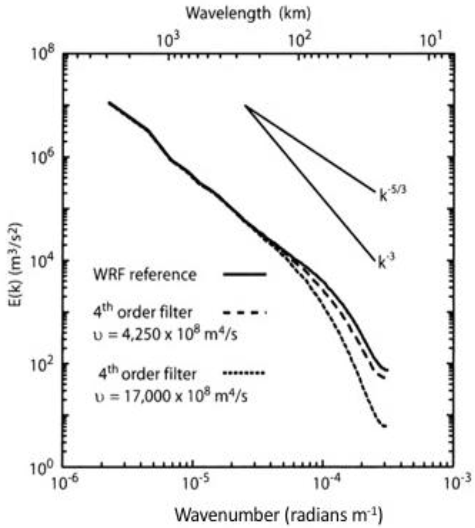
Models aim to replicate these spectra; departure from these curves at a particular wavelength indicates the simulated atmospheric velocities do not have the observed amount of energy at that scale of motion. For example, Figure 2 shows modeled atmospheric energy spectra from a simulation using the WRF model [47] using options producing relatively little dissipation. The energy spectrum compares well with the natural spectra at mesoscales, however, contains 10–100 times less energy than nature at the right side of the curve, in the fine-scale (high wave number, short wavelength) motions. The “effective resolution” of a simulation is defined as the wavelength below which the simulated spectrum begins to decay relative to the natural spectra [47]; their divergence intensifies at the scale where the larger-scale motions resolved by the model transition to turbulence treated by subgrid-scale parameterizations.
The downward cascade of energy to smaller scales in NWP models encompasses physical processes such as diffusion, numerical effects that arise from the choice of discretization schemes, and model filters that smooth and selectively eliminate specific scales of motion. The results are to reduce the energy in resolved motions, smooth gradients, and transport energy to fine scale motions where it is ultimately dissipated. Some dissipation at the finest scales is necessary both to reproduce the natural effect and because the downscale energy transfer would otherwise create an unrealistic accumulation of energy. It is also desirable from a practical perspective to suppress the buildup of numerical instabilities, rapid buildups of errors that prematurely terminate a simulation. However, cumulative dissipation (both physical and numerical) can be excessive and cause the modeled energy spectra to vary from the natural −5/3 energy spectra, particularly at the finest scales such as atmospheric motions at the scale of a few grid cells. Likewise, excessive diffusion of scalar variables would reduce gradients in scalars such as buoyancy between adjacent grid cells. Motions with spatial scales finer than the effective resolution are damped relative to the natural spectra and their energy is missing from the simulation. In practical terms, the divergence of the WRF simulation kinetic energy spectra in Figure 2 from the natural means that its wind fields lack small-scale structure, appear unnaturally smooth, and underestimate fluctuations. Simulated local air circulations would be weaker than observed or not captured.
As [47] notes, model spectra can be affected by model damping, and the finest resolvable modes are strongly dependent on the formulation and tuning of implicit and explicit model filters. In mesoscale modeling applications, disproportionate damping of the finest resolved scale motions is desirable to diminish small perturbations that are not of physical interest and which would amplify to cause numerical instabilities, particularly in complex terrain. However, in other applications, notably those where the phenomenon of interest arises and grows from gradients across adjacent cells—the impact is severely detrimental. Phenomena forced upscale—notably, fire motions arising from buoyancy gradients across a narrow fire line—or occurring at those scales—for example, fire whirls—will not be captured well. Adjustment of model filters, less dissipative closure schemes, or configuration as an LES can lessen dissipation at fine scales to some extent, but these are not practical or appropriate at convective to mesoscale scales, particularly for real cases, and can leave a simulation unable to continue in complex terrain due to the buildup of numerical errors [personal observation]. However, increasing viscous dissipation to manage the buildup of numerical errors can alter the simulated flow regimes. For example, in simulations of the Esperanza fire [17], increasing numerical diffusion caused airflow through Banning Pass to spread up onto slopes, where it drove a fire leading to five fatalities, whereas simulations with less diffusion caused the strong winds to remain within the pass. Other numerical methods have different properties that avoid this conundrum. For example, the alternate transport scheme Multidimensional Positive Definite Advection Transport Algorithm (MPDATA) [48], included in the Coupled Atmosphere-Wildland Fire Environment Model (CAWFE) model [49], was designed to reduce the implicit viscosity while reducing the reliance on numerical filters to maintain stability in simulations of geophysical fluid flow.
4.4. Terrain
Terrain shape is important for fire behavior modeling in two ways. It can determine the airflow regime in which a fire occurs. Examples include simulations of the Esperanza fire [17] in which supercritical flow—a fast, shallow airflow caused by a certain combination of terrain aspect ratio, high wind speed, and near surface stable air layers—drove the fire down the lee side of Cabazon Peak, setting up a run up a drainage that led to firefighter fatalities. In addition, inclined terrain directly increases fire propagation rate [50]. Notable fire behavior has occurred in the lee of ridges. A critical difference in fire behavior occurs if airflow separates from terrain in the lee or forms lee vortices and, absent propagation by burning embers, fire progression may be stopped if a fire will not descend or be driven downslope.
Considerations for applying NWP models of varying scales over complex terrain are discussed by [51]. Increasing NWP model resolution produces steeper slopes. Sharp elevation changes or very steep slopes challenge NWP models, creating disturbances near the earth’s surface that create numerical instabilities and reduce accuracy. To fix this, numerical filters are employed to smooth terrain bumpiness but, as previously noted, can change the airflow regime in complex ways. Most modeling systems standardly employ numerical filters on terrain elevation. These filters primarily smooth mountain peaks and valley lows but have little effect on steep slopes, another primary source of numerical instability, for which methods are being developed in WRF such as the immersed boundary method [52]. The CAWFE model, built upon the Clark-Hall atmospheric model optimized for use at very high resolution (100 s of m) in steep mountainous terrain, allows the user to filter either or both terrain elevation and the terrain gradient. In addition, CAWFE’s pressure solver, described in [53], forces the residual numerical divergence to remain at minimal levels. These adaptations have allowed CAWFE computations to continue when terrain slope is as much as 40°, a crucial capability when fires travel through mountainous terrain containing sharp canyons.
4.5. Solution Methods
Numerical solution of discretized versions of the set of fluid dynamics equations described in Section 3 for CFD-based fire behavior modeling systems generally follows one of two approaches, the choice of which produces different benefits and challenges. Some modeling systems (FIRETEC and coupled systems based upon WRF) use a compressible system, in which air density is a three-dimensional prognostic variable. A prognostic equation for density that requires very small time steps completes the system. Alternatively, in the anelastic approximation [54] that underlies CAWFE, while the background density may vary with height, density fluctuations appear only in buoyancy terms. Solution of this ‘anelastic’ system requires solving an elliptic partial differential equation for pressure, which is considered an expensive computation, however, the inclusion of a numerical divergence term guarantees mass conservation at each step. And, as systems using the anelastic approximation do not support sound waves, they can use much larger time steps. A negative impact of the anelastic approximation is that even though the fire’s temperature signal in coupled weather-fire models is that of buoyancy—tens of degrees Celsius—rather than the combustion temperature, extreme temperature deviations do not meet the validity of the anelastic model assumptions and truncate the most extreme vorticities that might be produced. The compressible form of the governing equations does not assure mass continuity to machine error at each time step and would soon lead to numerical instability and early model termination. In practice, systems such as WRF also add a numerical divergence term during integration to better conserve mass and perform several mini-time steps iterating density during each model time step, increasing the computational cost. Time splitting filters included in WRF to mitigate the impacts from compressible formulation produced numerical damping on the smallest scales of motion [55] and, though these scales would generally be of less meteorological interest [55], this dampening of fine scale motions damages the simulation of phenomena such as fires that build up from fine scales, as discussed in Section 4.3.
5. Configuration Considerations
Successful weather simulations resolve the physical processes responsible for producing air accelerations at appropriate scales of motion, supported by suitable numerical algorithms. User decisions about the grid’s size and shape can greatly influence simulated fire behavior.
5.1. Resolution
Coupled models have the potential to enhance the ability to understand and anticipate more complex, rapidly changing aspects of fire behavior provided that: (1) they resolve the intricate, time-varying airflow in mountainous terrain; and (2) they capture fire-atmosphere feedbacks responsible for fire-induced winds. Physics fidelity demands horizontal grid spacing on the order of one hundred meters [56,57] to capture fine-scale atmospheric circulations amid complex terrain and delineate fire-induced circulations, the effects of which are noticeably diluted at grid spacing of approximately 1 km or greater [58]. For comparison, this is more than an order of magnitude finer than current U.S. operational numerical weather prediction models.
Computational cost has been cited as a barrier to using NWP-based fire behavior models as forecasting tools [29], however, widespread access to supercomputing resources has enabled researchers to demonstrate computations for a large wildland fire with a WRF-based coupled model using 500 m grid spacing [59] at speeds that broach faster than real time using 120 processors, or for smaller fires, produce an 18 h forecast in ~4 h on 24 processors [60]. Other models have better performance and, posing a different forecasting paradigm, achieve simulations several times faster than real time in single processor calculations on workstations (pers. observation)—a more widely accessible platform. Instead, issues pertaining to resolution impact the simulations’ quality.
As noted in Section 4.3, motions with spatial scales finer than the resolution at which the energy spectrum begins to decay relative to the natural spectra are damped and their energy is missing from the simulation. In WRF simulations, Ref. [47] noted that this excessive numerical damping produced an “effective resolution” that was seven times the grid spacing. It was recommended elsewhere [61] that WRF be used at horizontal grid spacings greater than 2 km.
5.2. Grid Aspect Ratio
An additional issue related to resolution is the grid aspect ratio, the ratio of the vertical grid cell length to the horizontal grid cell length. Convective-scale and large eddy simulation modeling simulate air flow characterized by tilting of motions between horizontal and vertical directions. Accuracy is best maintained when the vertical to horizontal grid aspect ratio is ~1, that is, the grid volume is an equal-sided cube. Good practice for convective-scale and turbulence modeling maintains the aspect ratio between 1 and 5 [38]. This is critical for fire modeling as sharp buoyancy gradients across narrow fire lines perhaps tens of meters wide and convective updrafts that tilt the rotation into the vertical are the source of fire-induced motions. A gradient may be resolved in 10-m vertical grid spacing, under-resolved when rotated and spread across, for example, 100-m horizontal grids, and resampled again when rotated again into the vertical. Tilting between resolved and unresolved dimensions creates what appears to be fine-scale motions but is instead numerical noise—spurious motions arising from inappropriate configuration. For fires, this is particularly important near the surface, but may also impact the simulation of other fire effects—such as the mixing between a fire plume and ambient air—at higher elevations.
Maintaining this grid aspect ratio in the range of good practice imposes further needs on model development. NWP models commonly refine horizontal grids during grid nesting as modeling domains telescope from horizontal grid spacing of 10 s of km to a resolution appropriate for modeling the phenomena of interest—here, 100 s of meters. Less common is the capability to refine vertical grids. If a single vertical grid must be used for all nested domains, it is difficult to maintain the grid aspect ratio within the good practice range while having the high resolution needed near the surface and very small time steps needed to keep numerically stable over complex terrain.
Models such as CAWFE employ vertical as well as horizontal grid refinement [62] enabling grid nesting and refinement down to convective modeling scales with less numerical noise generation. Nevertheless, NWP simulations of real cases are not nested from 10 s of km grid spacing to under ~100 m for reasons beyond the computational cost. Such fine grid spacing is typically used to study the atmospheric boundary layer, in which turbulence driven by buoyancy and shear stresses dominates the flow and cannot be modeled accurately in a deterministic manner.
5.3. Typical Configuration Paradigms
Wildland fire simulations typically address one of two fire scenarios—a large fire event or a small, prescribed fire. Each pose different challenges.
5.3.1. Large-Scale Simulations
Numerous studies (e.g., [15,17,56,57,58,59,63,64] and others) have applied coupled weather-fire models to simulate large wildland fire events. The standard approach, taken from NWP, is to begin with a regional model domain with the approximate grid spacing of a larger-scale forecast or analysis product, either of which may provide initial and boundary conditions (10–12 km). Then, simulations use grid nesting and (horizontal, and if available, vertical) refinement with increasingly fine resolution in 2–4 inner domains to reach 100–1000 m horizontal grid spacing. Users model the fire’s evolution within the finest-resolution domain.
This approach has served well when applied to fire events, however, the strong winds and complex terrain in which fires sometimes occur, the extreme winds sometimes produced by a fire, and the need to nest to O [100 m], make it difficult to conduct high quality simulations.
- Simultaneous requirements for good meteorological simulations can be mutually exclusive. For example, models such as WRF without vertical grid refinement must employ a stretched vertical grid that would ideally have fine vertical resolution near the surface, but which creates a low grid aspect ratio while nesting over 4–5 domains. Each domain must remain numerically stable while incorporating potentially high ambient and fire winds in steep, rough terrain without excessive smoothing of winds or terrain—a daunting challenge.
- Nested domains introduce flows into inner domains that have the coarser spatial scales of the parent domain. Modelers attempt to mitigate this by using large inner domains and assume that the distance from the boundary allows flows to spin up before reaching the area of interest. However, in practical terms, it is a limitation of limited area models that due to the time required, the inner domain does not fully develop the finer scales [65]. Attempts to introduce turbulence to flow at the inner domain boundary [66] address but have not completely fixed the issue and are not generally applicable.
- In forecasting applications (e.g., [60]) where domain sizes are limited to meet time constraints, flows in all domains may not fully develop and may appear to be boundary conditions interpolated onto the finer domain grid points.
5.3.2. Configuration for Small-Scale Fires
Small fires and other phenomena have been studied with both coupled atmosphere-fire models and coupled weather-fire models. Idealized studies have examined fine-scale fire phenomena such as fire whirls [16] and tested sensitivity to fire environment parameters [67]. Some studies attempt to reproduce real prescribed fires [68], often fires conducted during instrumented experiments [19,23,69,70], yet struggle with representing the ambient wind environment [69], which can vary over a small area, and small-scale atmospheric fluctuations [19]. Also, prescribed fires may be ignited with complex ignition patterns and tampered with over time, interfering with the fire’s natural evolution.
Simulating small fires such as prescribed fires presents challenges beyond large-scale events. These require model resolution at ten meters or less—well within the boundary layer regime. At this scale, airflow is generally dominated by small-scale fluctuations—shear- and surface heating and moisture-driven eddies—rather than distinct meteorological events. Properly configured idealized simulations with suitable models may illuminate some aspects of fire behavior interactions with a turbulent atmospheric boundary layer.
Preferably, simulation of idealized small fires would use turbulence models; existing approaches use NWP models designed for other scales configured in LES mode. Best practices using WRF are described by [67,71]. Single domain, idealized simulations are configured using cyclic boundary conditions, which take flow leaving the downwind face and reintroduce it upwind as inflow. Simulations are run one to several hours until a fully developed turbulent flow builds up, then a fire is ignited. This technique has limitations. It precludes topography, as terrain would create a flow disturbance that is reintroduced upwind of the hill that caused it. Also, a fire introduces thermal and momentum perturbations and smoke that would reenter the domain upwind of the fire itself—an unnatural effect.
Good practice advises against trying to reproduce real fires through single, purely deterministic simulations. Firstly, NWP simulations are not refined to 1–10 m not only because of computational cost but because of the inability to model weather deterministically at this scale. Secondly, a fire line’s encounter with an eddy could dominate its behavior yet the timing and location of eddies is unpredictable. Prescribed fire simulations in [19] suffer these weaknesses. They noted difficulties reproducing observed fire growth with wind fluctuations of the same magnitude as the mean wind speed and that the poorly resolved atmospheric turbulence significantly influenced parts of the evolving fire line, making details of fire behavior difficult to reproduce.
6. Specific Scenarios
Simulation of a fire incident, including how it unfolds with time and the production of fire phenomena, requires that the user accurately simulate the weather event in which it occurs, yet some weather events associated with fires are among the most difficult to model accurately. This can be because the weather event’s predictability is inherently limited or a specific model’s accuracy is limited by issues listed in Section 4 and Section 5.
Numerous deaths have been tied to fires directed by convective clouds, precipitation, and resulting gust fronts such as the 2013 Yarnell Hill Fire, the 1990 Dude Fire, and the 2015 Frog Fire and mesoscale convective system outflow of the 2012 Waldo Canyon Fire. Anticipating these events has eluded early fire behavior models and coupled atmosphere-fire models without a weather component; success with coupled weather-fire models inextricably depends on modeling convection initiation, precipitation, and associated outflows accurately. When convection is triggered by a topographic feature and models capture topographic shaping of the flow, the lifting of moist air, and subsequent cloud, rainfall, and outflow production, reproducing the impact on fire behavior is potentially feasible, for example, a CAWFE simulation of the Yarnell Hill event case reproduced two wind shifts and impacts on fire direction and intensification [12]. Aside from topographically tied events, the specific location and timing of convective initiation on flat terrain is difficult to predict more than an hour ahead of time [R. Roberts, pers. comm.]. The predictability of gust front behavior, particularly in complex terrain, and its impact on fire behavior has been identified as a fire community research need [72].
Downslope windstorms have fueled some of the most destructive fire events in Colorado and northern and southern California. In Colorado, wind event-driven fires are primarily associated with unseasonal windstorms, driven by breaking atmospheric gravity waves (e.g., the 2012 High Park Fire [56]. Southern California windstorm-driven fires are associated with Santa Anas—seasonal pressure-driven offshore flows—and sundowners. Curiously, although the phenomenon has long been recognized (i.e., [27]) simulations of the structure of Santa Anas (e.g., [73]) and Santa Ana-driven fire events (e.g., [17,59]) have been overlooked until recently. Similarly, the Diablo winds of northern California have historically driven some of the most destructive events (e.g., the 1991 Oakland Hills fire and the 2017 Napa and Sonoma County fires) but other than general descriptions of cause and appearance, have not been modeled in fine detail. In both Santa Anas and Diablo winds, meteorological data in areas experiencing peak wind speeds are sparse yet suggest comparable extreme peak winds to Colorado Front Range windstorms (approximately 30–40 m s−1).
Important elements of all three events (Front Range windstorms, Santa Anas, and Diablo winds) are the broad regional wind patterns and the peak winds, which may sometimes contribute to a fire’s ignition as well as early rapid growth, enabling it to escape initial attack. WRF simulations well represented regional wind patterns and time series of winds at surface weather stations downwind of the peak winds but underestimated the peak winds themselves [74]. For example, [74] increase their simulated winds at peak speed locations by 30–50%, using the gust factor as scaling factor, to meet observed wind speeds. This discrepancy has been underemphasized in the literature and its causes not discussed. Other work [56] using the convective-scale model CAWFE reproduced gravity wave overturning, a phenomenon underlying previous Front Range windstorm events, during the High Park Fire. They noted that in other studies, other models failed to reproduce the overturning waves, characterized by fine-scale temperature and velocity gradients, creating only some vertical displacement and surface wind acceleration in the lee, and typically underestimated peak wind speeds. These discrepancies appear to arise from the factors cited in Section 4 and Section 5, notably the resolution (as breaking waves only appeared using horizontal grid spacing under 300 m [56] while [74] used 667 m and [59] used 500 m); excessive dissipation at fine scales in WRF; and flow distortion when along-terrain gradients are tilted into the vertical.
Fire phenomena are impacted by the issues raised in Section 4 and Section 5 as well. For example, fire whirls are produced when a horizontal buoyancy gradient across the fire line is tilted into the vertical by convective updrafts produced by the fire. Reproducing this effect requires a low grid aspect ratio otherwise the motion generates excessive numerical noise. Excessive dissipation at fine scales smooths out these fine gradients and distorts the development of larger-scale motions. Weaknesses in the ability to meet these criteria explain the unnaturally weak vortices produced by [15] (in contrast to [16], where WRF is configured in LES mode or [9]), despite ample heat fluxes along a shear zone—prime conditions for fire whirl formation.
As noted in Section 5, complex terrain creates disturbances in simulated thermodynamic and velocity fields that can reduce accuracy and amplify into numerical instabilities that terminate simulations. Modelers typically address this with additional filters on model terrain or elevation gradients and numerical filters. While not of meteorological interest in mesoscale applications, microscale topographic features that would not appear at mesoscale model resolutions (2 km and up) or be greatly smoothed out can interrupt fire spread. Also, whether winds penetrate down into narrow canyons and drainages can determine whether a fire progresses. In addition, the simulated daytime slope and valley wind system, an important factor in fire weather, varies from one mesoscale model to another [75]. They note large differences in local flow evolution, particularly near the surface, primarily in the time of onset due to differences in terms calculated in the surface energy budget. That wildfires typically traverse mountainous terrain and valleys while requiring undamped, resolved microscale simulations (~100 m–300 m) presents a modeling challenge.
In summary, some uncertainty or apparent unpredictability in modeling fire behavior with coupled models arises from genuine uncertainties in atmospheric prediction in certain conditions, however, physical understanding and the ability to predict fire phenomena and events has in fact advanced. In addition, coupled models present a framework to investigate remaining issues, such as the role that lofting and transport of burning embers [76] plays in the propagation of fires. Many limitations in studies to date arise from using modeling systems based on atmospheric models designed for a different scale and which lack suitable features and numerical properties. Section 7 discusses methods readers may use to identify and attribute inadequate outcomes and methods modelers may be using surreptitiously to adjust or fix them.
7. Addressing Inadequate Outcomes
Previous sections describe model design, configuration limitations, and their consequences. Knowing these beforehand, users can more efficiently recognize and perform well-designed experiments. However, these requirements have not always been recognized nor adhered to, resulting in errors in the modeled wind field that have harmed fire behavior simulations or reduced the ability to reproduce fire phenomena, some of which are important for firefighter safety. Meanwhile, techniques have arisen and spread widely, becoming unquestioned, that reconcile or adjust inadequate outcomes to observations or expected outcomes. Or, by misinterpreting the error’s cause, they misdirect further development aimed at fixing it. Some examples are the following:
- Misattribution of errors, leading toward more model complexity. In NWP models, for example, incorrect velocity fields can create overly vigorous or weak convective clouds, and alter the precipitation the simulations produce. Modelers can misattribute this to weaknesses in the cloud physics parameterizations, suggesting more detailed physical parameterizations are required. In fire behavior modeling using early kinematic models, failure to incorporate the spatially and temporally varying wind and fire-induced winds in simulations contributed to errors in the simulated rate of spread. This inadequacy led to more complex fuel classification systems and adjustments to rate of spread formulae.
- Calibration—changing simulation inputs. Errors in predicted rate of spread using operational fire behavior models such as BEHAVE or FARSITE have been addressed by incorporating spread rate adjustment factors [5,77] that allow the user to tune the simulation to observed fire spread patterns and by ad hoc manual calibrations. In the latter, when fuel, weather, and terrain inputs generate an incorrect estimate of rate of spread, users are advised to note observed fire behavior and adjust inputs and rerun simulations until the simulation is consistent with field observations [78], noting calibration factors for use in later simulations. While operationally useful, the need for such calibration indicates the underlying scientific model is flawed.
- Calibration—adjusting simulation outputs. Meteorologists define the gust factor as the ratio of the peak wind speed over a given time period to the mean wind speed. They are used to account for and estimate wind variability and extrema that measurements may miss. Gust factors have also been applied to NWP mesoscale models to estimate underresolved wind extrema. For example, the authors of [74] apply gust factors of 1.3–2.0 to their simulated winds to match peak winds during the Santa Ana driving the Witch Fire. Used in conditions that violate assumptions made during gust factors’ derivation and outside the phenomena for which they were derived, they instead may be used to rationalize inflating simulated winds to observed values. This calibration thus encompasses not only the real, natural variability of wind speeds but also simulation shortcomings that arise due to not resolving motions and the dissipation of sharp gradients at small scales. Also, [79] present another calibration to correct WRF wind speed biases over complex terrain.
- Calibration factors—the wind adjustment factor. Recognizing that wind speed decreases between a Remote Automated Weather Station’s height and the surface, [80] devised an adjustment factor to vertically adjust measured wind speeds to the mid-flame height for use in rate of spread calculations. However, NWP models already reproduce this effect with surface layer parameterizations or directly through treatment of the surface stress and shear energy dissipation terms. Thus, including the wind adjustment factor in coupled weather-fire models has no physical meaning. Implemented in WRF-SFIRE [81], this adjustment, not mentioned in later publications, is used to calibrate simulated fire rate of spread toward observations.
The need for and use of such factors should be considered when critically interpreting simulation results. Normalizing these techniques obscures underlying model inadequacies. Encouraging development of diverse models prevents the limitations of a specific model or model class being misinterpreted as unavoidable or fire being labelled as innately unpredictable.
8. Discussion
Within the wildland fire community, models of varying complexity are used to simulate fire behavior and wind, one of fire behavior’s primary influencers. Depending on the purpose of the simulation, simple models may meet users’ needs in certain conditions, such as where behavior is foreseeable and uncomplicated. Coupled atmosphere-fire models have emerged as tools that may expand our ability to understand and predict more complex and rapidly-changing aspects of fire behavior, however, their limitations, additional requirements, and configuration should be understood. Incorrectly selected or applied, models may omit or distort phenomena, not capture the evolving fire perimeter shape without correction factors, create erroneous circulations, and make fire behavior appear unpredictable.
Different types of coupled models have different strengths. NWP-based coupled models necessarily parameterize fire physical processes, but capture atmospheric and land surface processes shaping winds—arguably the most important factors shaping landscape-scale fires. In contrast, though CFD-fire models such as FIRETEC and WFDS distinguish combustion processes and fuel structure with greater detail, making them good tools for investigating the effect of vegetation structure on local fire behavior in idealized experiments, they lack components to model weather, making them unsuitable for landscape-scale fires, computational needs aside. The idea of linking models designed for different scales (such as nesting FIRETEC within a weather model) is not new. Faced with the need to represent the effects of boundary layer turbulence on atmospheric processes, [65] explored possible methods to link a large-eddy simulation model domain with a weather forecast model. They discussed how this linkage, which seemed straightforward, presented difficult issues, including spin-up in the inner domain and outcomes between the different model domains’ physics that did not match.
Even among coupled weather-fire models, tools can have greatly different capabilities and properties. Models based on convective-scale NWP models such as CAWFE have an advantage in that the underlying NWP model was designed to simulate weather in steep, complex terrain and maintain sharp variable gradients. In contrast, WRF, a mesoscale model, aggressively dissipates fine-scale motions and gradients, distorting the evolving fire perimeter and strongly dampening the fire signature because sharp gradients are smoothed as they attempt to form fire phenomena and build up to convective scales. It lacks the flexibility to accurately capture fine-scale gradients and rotation and underpredicts peak winds in downslope windstorms, the extreme meteorological events behind some of the most destructive fire incidents. WRF-based model users may be caught between bounding limitations, as attempting to reduce dissipation and filters enables instabilities triggered by highly complex terrain to disrupt simulations. In addition, some scenarios remain out of reach of all models. For example, the evolution of real, small, prescribed fires is inherently difficult and no well-founded approach exists due to the inability to deterministically predict turbulent atmospheric boundary layer motions in real conditions at the appropriate scales.
Users from disciplines outside the physical sciences may seek new knowledge to use, configure, and interpret simulations from coupled models, however some concepts presented here may also be new to atmospheric modelers. Coupled weather-fire modeling has requirements different from other weather modeling areas, such as mesoscale meteorology, yet the issues described here may also negatively impact simulations of other phenomena. As noted, dissipation limits peak winds in mesoscale simulations of downslope winds. Smoke modeling is negatively impacted as well [40]. Numerous meteorological phenomena also arise from small-scale temperature gradients. Precipitation formation in complex terrain is negatively impacted by errors in fine-scale winds, with subsequent impacts on forecasted hydrometeorology, which may be used to anticipate post-fire mudslides. Recognizing these modeling issues should enlighten modelers on source of errors that currently are otherwise attributed to natural uncertainty and unpredictability.
Acknowledgments
This work was supported by the National Aeronautics and Space Administration (NASA) under award NNX12AQ87G and the Federal Emergency Management Agency under award EMW-2015-FP-00888. The National Center for Atmospheric Research is sponsored by the National Science Foundation (NSF). Any opinions, findings, and conclusions or recommendations expressed in this material are the author’s and do not reflect the views of NSF. I thank Peter Sullivan for helpful discussions on boundary layer modeling. Comments from anonymous reviewers greatly improved the manuscript.
Conflicts of Interest
The author declares no conflicts of interest.
References
- Rothermel, R.C. A Mathematical Model for Predicting Fire Spread in Wildland Fuels; Research Paper INT-115; USDA Forest Service, Intermountain Forest and Range Experiment Station: Ogden, UT, USA, 1972.
- Wolff, M.F.; Carrier, G.F.; Fendell, F.E. Wind-aided firespread across arrays of discrete fuel elements. II. Experiment. Combust. Sci. Technol. 1991, 77, 261. [Google Scholar] [CrossRef]
- Fendell, F.E.; Wolff, M.F. Chapter 6: Wind-aided fire spread. In Forest Fires—Behavior and Ecological Effects; Johnson, E.A., Miyanishi, K., Eds.; Academic Press: San Diego, CA, USA, 2001; pp. 171–223. [Google Scholar]
- Richards, G.D. An elliptical growth model of forest fire fronts and its numerical solution. Int. J. Numer. Methods Eng. 1990, 30, 1163–1179. [Google Scholar] [CrossRef]
- Finney, M.A. FARSITE: Fire Area Simulator—Model Development and Evaluation; US Forest Service: Ogden, UT, USA, 1998.
- Noonan-Wright, E.; Opperman, T.S.; Finney, M.A.; Zimmerman, T.G.; Seli, R.C.; Elenz, L.M.; Calkin, D.E.; Fiedler, J.R. Developing the U.S. Wildland Fire Decision Support System (WFDSS). J. Combust. 2011. [Google Scholar] [CrossRef]
- Ramirez, J.; Monedero, S.; Buckley, D. New approaches in fire simulations analysis with wildfire analyst. In Proceedings of the 5th International Wildland Fire Conference, Sun City, South Africa, 9–13 May 2011. [Google Scholar]
- Clark, T.L.; Jenkins, M.A.; Coen, J.; Packham, D. A Coupled Atmospheric-Fire Model: Convective Feedback on Fire Line Dynamics. J. Appl. Meteorol. 1996, 35, 875–901. [Google Scholar] [CrossRef]
- Clark, T.L.; Jenkins, M.A.; Coen, J.; Packham, D. A Coupled Atmospheric-Fire Model: Convective Froude number and Dynamic Fingering. Int. J. Wildland Fire 1996, 6, 177–190. [Google Scholar] [CrossRef]
- Linn, R.R. A Transport Model for Prediction of Wildfire Behavior. Ph.D. Thesis, New Mexico State University, Las Cruces, NM, USA, 1997. [Google Scholar]
- National Fire Academy. 2nd National Fire Service Research Agenda Symposium Report. National Fallen Firefighters Foundation. 2011. Available online: http://www.everyonegoeshome.com/symposium/report2.pdf (accessed on 12 December 2017).
- Coen, J.L.; Schroeder, W. Coupled Weather-Fire Modeling: From Research to Operational Forecasting. Fire Manag. Today 2017, 75, 39–45. [Google Scholar]
- Jenkins, M.A.; Clark, T.; Coen, J. Chapter 8: Coupling Atmospheric and Fire Models. In Forest Fires—Behavior and Ecological Effects; Johnson, E.A., Miyanishi, K., Eds.; Academic Press: San Diego, CA, USA, 2001; pp. 171–223. [Google Scholar]
- Clark, T.L.; Coen, J.L.; Latham, D. Description of a Coupled Atmosphere-Fire Model. Int. J. Wildland Fire 2004, 13, 49–63. [Google Scholar] [CrossRef]
- Peace, M.; Mattner, T.; Mills, G.; Kepert, J.; McCaw, L. Fire-modified meteorology in a coupled fire-atmosphere model. J. Appl. Meteorol. Clim. 2015, 54, 704–720. [Google Scholar] [CrossRef]
- Simpson, C.C.; Sharples, J.J.; Evans, J.P. Resolving vorticity-driven lateral fire spread using the WRF-Fire coupled atmosphere-fire numerical model. Nat. Hazards Earth Syst. Sci. 2014, 14, 2359–2371. [Google Scholar] [CrossRef]
- Coen, J.L.; Riggan, P.J. Simulation and thermal imaging of the 2006 Esperanza wildfire in southern California: Application of a coupled weather-wildland fire model. Int. J. Wildland Fire 2014, 23, 755–770. [Google Scholar] [CrossRef]
- Hoffman, C.; Morgan, P.; Mell, W.; Parsons, R.; Strand, E.K.; Cook, S. Numerical simulation of crown fire hazard immediately after bark beetle-caused mortality in lodgepole pine forests. For. Sci. 2012, 58, 178–188. [Google Scholar] [CrossRef]
- Linn, R.R.; Winterkamp, J.; Furman, J.; Williams, B. Simulating low-intensity experimental fires using a coupled fire-atmosphere behavior model. In Proceedings of the 11th Conference of Fire and Forest Meteorology, Minneapolis, MN, USA, 4–7 May 2015. [Google Scholar]
- Warner, T.T. Quality assurance in atmospheric modeling. Bull. Am. Meteorol. Soc. 2011, 1601–1610. [Google Scholar] [CrossRef]
- Bachelor, G.K. Introduction to Fluid Dynamics; Cambridge University Press: Cambridge, UK, 1967. [Google Scholar]
- Roache, P.J. Computational Fluid Dynamics; Hermosa Publishers: Albuquerque, NM, USA, 1985. [Google Scholar]
- Mell, W.E.; Jenkins, M.A.; Gould, J.S.; Cheney, N.P. A physics-based approach to modeling grassland fires. Int. J. Wildland Fire 2007, 16, 1–22. [Google Scholar] [CrossRef]
- Mell, W.; Maranghides, A.; McDermott, R.; Manzello, S.L. Numerical simulation and experiments of burning Douglas fire trees. Combust. Flame 2009, 156, 2023–2041. [Google Scholar] [CrossRef]
- Blumen, W. Atmospheric Processes over Complex Terrain; American Meteorological Society: Boston, MA, USA, 1990; Volume 23. [Google Scholar]
- Baines, P.G. Topographic Effects in Stratified Flows; Cambridge University Press: New York, NY, USA, 1997. [Google Scholar]
- Whiteman, C.D. Mountain Meteorology: Fundamentals and Applications; Oxford University Press: New York, NY, USA, 2000. [Google Scholar]
- Shaw, R.H.; Schumann, U. Large-eddy simulation of turbulent flow above and within a canopy. Bound-Layer Meteorol. 1992, 61, 47–64. [Google Scholar] [CrossRef]
- Forthofer, J.M.; Butler, B.W.; Wagenbrenner, N.S. A comparison of three approaches for simulating fine-scale surface winds in support of wildland fire management. Part I. Model formulation and comparison against measurements. Int. J. Wildland Fire 2014, 23, 969–981. [Google Scholar] [CrossRef]
- Forthofer, J.M.; Butler, B.W.; McHugh, C.W.; Finney, M.A.; Bradshaw, L.S.; Stratton, R.D.; Shannon, K.S.; Wagenbrenner, N.S. A comparison of three approaches for simulating fine-scale surface winds in support of wildland fire management. Part II. An exploratory study of the effect of simulated winds on fire growth simulations. Int. J. Wildland Fire 2014, 23, 982–994. [Google Scholar] [CrossRef]
- Castro, F.A.; Palma, J.M.L.M.; Silva Lopes, A. Simulation of the Askervein flow. Part 1: Reynolds averaged Navier-Stokes equations (K–E turbulence model). Bound-Layer Meteorol. 2003, 107, 501–530. [Google Scholar] [CrossRef]
- Butler, B.W.; Wagenbrenner, N.S.; Forthofer, J.M.; Lamb, B.K.; Shannon, K.S.; Finn, D.; Eckman, R.M.; Clawson, K.; Bradshaw, L.; Sopko, P.; et al. High-resolution observations of the near-surface wind field over an isolated mountain and in a steep river canyon. Atmos. Chem. Phys. 2015, 15, 3785–3801. [Google Scholar] [CrossRef]
- Lorenz, E.N. The predictability of a flow which possesses many scales of motion. Tellus 1969, 21, 289–307. [Google Scholar] [CrossRef]
- Lilly, D.K. Numerical prediction of thunderstorms—Has its time come? Q. J. R. Meteorol. Soc. 1980, 116, 779–798. [Google Scholar]
- Dalcher, A.; Kalnay, E. Error growth and predictability in operational ECMWF forecasts. Tellus 1987, 39, 474–491. [Google Scholar] [CrossRef]
- Mukherjee, S.; Schalkwuk, J.; Jonker, H.J.J. Predictability of dry convective boundary layers: An LES study. J. Atmos. Sci. 2016, 73, 2715–2727. [Google Scholar] [CrossRef]
- Moeng, C.-H. A large-eddy-simulation model for the study of planetary boundary-layer turbulence. J. Atmos. Sci. 1984, 41, 2052–2062. [Google Scholar] [CrossRef]
- Sullivan, P.P.; Patton, E.G. The effect of mesh resolution on convective boundary layer statistics and structures generated by large-eddy simulation. J. Atmos. Sci. 2011, 68, 2395–2415. [Google Scholar] [CrossRef]
- Moeng, C.-H.; Dudhia, J.; Klemp, J.; Sullivan, P. Examining two-way grid nesting for large eddy simulation of the PBL using the WRF model. Mon. Weather Rev. 2007, 135, 2295–2311. [Google Scholar] [CrossRef]
- Gibbs, J.A.; Federovich, E. Comparison of convective boundary layer velocity spectra retrieved from large-eddy-simulation and Weather Research and Forecasting model data. J. Appl. Meteorol. Clim. 2014, 53, 377–394. [Google Scholar] [CrossRef]
- Sullivan, P.P.; McWilliams, J.C.; Moeng, C.-H. A subgrid-scale model for large-eddy simulation of planetary boundary-layer flows. Bound-Layer Meteorol. 1994, 71, 247–276. [Google Scholar] [CrossRef]
- Haines, D.A.; Smith, M.C. Three types of horizontal vortices observed in wildland mass and crown fires. J. Clim. Appl. Meteorol. 1987, 26, 1624–1637. [Google Scholar] [CrossRef]
- Coen, J.L.; Mahalingam, S.; Daily, J.W. Infrared imagery of crown-fire dynamics during FROSTFIRE. J. Appl. Meteorol. 2004, 43, 1241–1259. [Google Scholar] [CrossRef]
- Luderer, G.; Trentmann, J.; Andreae, M.O. The role of fire-released moisture on the dynamics of atmospheric pyro-convection. Int. J. Wildland Fire 2009, 18, 554–562. [Google Scholar] [CrossRef]
- Graham, R.T. Hayman Fire Case Study; Department of Agriculture, Forest Service, Rocky Mountain Research Station: Ogden, UT, USA, 2003.
- Nastrom, G.D.; Gage, K.S. A climatology of atmospheric wavenumber spectra of wind and temperature observed by commercial aircraft. J. Atmos. Sci. 1985, 42, 950–960. [Google Scholar] [CrossRef]
- Skamarock, W.C. Evaluating mesoscale NWP models using kinetic energy spectra. Mon. Weather Rev. 2004, 132, 3019–3032. [Google Scholar] [CrossRef]
- Smolarkiewicz, P.K.; Margolin, L.G. MPDATA: A finite-difference solver for geophysical flows. J. Comput. Phys. 1998, 140, 459–480. [Google Scholar] [CrossRef]
- Coen, J.L. Modeling Wildland Fires: A Description of the Coupled Atmosphere-Wildland Fire Environment Model (CAWFE); NCAR Technical Note NCAR/TN-500+STR; NCAR: Boulder, CO, USA, 2013. [Google Scholar]
- Pyne, S.J.; Andrews, P.L.; Laven, R.D. Introduction to Wildland Fire, 2nd ed.; Wiley: New York, NY, USA, 1996. [Google Scholar]
- Zhong, S.; Chow, F. Meso- and fine-scale modeling over complex terrain: Parameterizations and applications. In Mountain Weather Research and Forecasting, Recent Progress and Current Challenges; Springer Atmospheric Sciences: Dordrecht, The Netherlands, 2013; pp. 591–653. [Google Scholar]
- Lundquist, K.A.; Chow, F.K.; Lundquist, J.K. An immersed boundary method for the weather research and forecasting model. Mon. Weather Rev. 2010, 138, 796–816. [Google Scholar] [CrossRef]
- Clark, T.L. Block-iterative method of solving the nonhydrostatic pressure in terrain-following coordinates: Two-level pressure and truncation error analysis. J. Appl. Meteorol. 2003, 42, 970–983. [Google Scholar] [CrossRef]
- Ogura, Y.; Phillips, N.A. Scale analysis of deep and shallow convection in the atmosphere. J. Atmos. Sci. 1962, 19, 173–179. [Google Scholar] [CrossRef]
- Skamarock, W.C.; Klemp, J.B. The stability of time-split numerical methods for the hydrostatic and the nonhydrostatic elastic equations. Mon. Weather Rev. 1992, 120, 2109–2127. [Google Scholar] [CrossRef]
- Coen, J.L.; Schroeder, W. The High Park Fire: Coupled weather-wildland fire model simulation of a windstorm-driven wildfire in Colorado’s Front Range. J. Geophys. Res. Atmos. 2015, 120, 131–146. [Google Scholar] [CrossRef]
- Coen, J.L.; Stavros, E.N.; Fites-Kaufman, J.-A. Deconstructing the King megafire. Ecol. Appl. 2017. under review. [Google Scholar]
- Coen, J.L. Simulation of the Big Elk Fire using coupled atmosphere-fire modeling. Int. J. Wildland Fire 2005, 14, 49–59. [Google Scholar] [CrossRef]
- Kochanski, A.K.; Jenkins, M.A.; Mandel, J.; Beezley, J.D.; Krueger, S.K. Real time simulation of 2007 Santa Ana fires. For. Ecol. Manag. 2013, 294, 136–149. [Google Scholar] [CrossRef]
- Kosovic, B.; Mahoney, W.P.; Brown, B.G.; Cowie, J.R.; Anderson, A.; Boehnert, J.; Bresch, J.; Jimenez, P.A.; Munoz-Esparza, D.; Petzke, W.; et al. Advancements in Operational Wildland Fire Prediction; NCAR Day of Networking and Discovery 2017; National Center for Atmospheric Research (NCAR): Boulder, CO, USA, 2017. [Google Scholar]
- Klemp, J.B. Advances in the WRF model for convection-resolving forecasting. Adv. Geosci. 2006, 7, 25–29. [Google Scholar] [CrossRef]
- Clark, T.L.; Farley, R.D. Severe downslope windstorm calculations in two and three spatial dimensions using anelastic interactive grid nesting: A possible mechanism for gustiness. J. Atmos. Sci. 1984, 41, 329–350. [Google Scholar] [CrossRef]
- Filippi, J.-B.; Bosseur, F.; Pialat, X.; Santoni, P.-A.; Strada, S.; Mari, C. Simulation of Coupled Fire/Atmosphere Interaction with the MesoNH-ForeFire Models. J. Combust. 2011. [Google Scholar] [CrossRef] [Green Version]
- Dahl, N.; Xue, H.; Hu, X.; Xue, M. Coupled fire-atmosphere modeling of wildland fire spread using DEVS-FIRE and ARPS. Nat. Hazards 2015, 77, 1013–1035. [Google Scholar] [CrossRef]
- Moeng, C.-H.; Weil, J. Turbulence Interaction with Atmospheric Physical Processes. In Turbulence and Interactions. Notes on Numerical Fluid Mechanics and Multidisciplinary Design; Deville, M., Lê, T.H., Sagaut, P., Eds.; Springer: Berlin/Heidelberg, Germany, 2010; Volume 110. [Google Scholar]
- Munoz-Esparza, D.; Kosovic, B.; Garcia-Sanchez, C.; van Beeck, J. Nesting turbulence in an offshore convective boundary layer using large eddy simulations. Bound-Layer Meteorol. 2014, 151, 453–478. [Google Scholar] [CrossRef]
- Coen, J.L.; Cameron, M.; Michalakes, J.; Patton, E.G.; Riggan, P.J.; Yedinak, K.M. WRF-Fire: Coupled Weather-Wildland Fire Modeling with the Weather Research and Forecasting Model. J. Appl. Meteorol. Clim. 2013, 52, 16–38. [Google Scholar] [CrossRef]
- Filippi, J.-B.; Pialat, X.; Clements, C.B. Assessment of FOREFIRE/MESONH for wildland fire/atmosphere coupled simulation of the FireFlux experiment. Proc. Combust. Inst. 2013, 34, 2633–2640. [Google Scholar] [CrossRef]
- Linn, R.; Anderson, K.; Winterkamp, J.; Brooks, A.; Wotton, M.; Dupuy, J.-L.; Pimont, F.; Edminster, C. Incorporating field wind data into FIRETEC simulations of the International Crown Fire Modeling Experiment (ICFME): Preliminary lessons learned. Can. J. For. Res. 2012, 42, 879–898. [Google Scholar] [CrossRef]
- Kochanski, A.; Jenkins, M.; Mandel, J.; Beezley, J.; Clements, C.B.; Krueger, S. Evaluation of WRF-Sfire Performance with Field Observations from the FireFlux Experiment. Geosci. Model Dev. 2013, 6, 1109–1126. [Google Scholar] [CrossRef]
- Coen, J.L. WRF-Fire: A Physics Package for Modeling Wildland Fires. WRF Users’ Tutorial. January 2015. Available online: http://www2.mmm.ucar.edu/wrf/users/tutorial/201501/FIRE.pdf (accessed on 12 December 2017).
- Joint Fire Science Program. Validating Mesoscale, Atmospheric Boundary Prediction Models and Tools. 2017. Available online: https://www.firescience.gov/AFPs/17-1-05/17-1-05_FON_Announcement.pdf (accessed on 15 December 2017).
- Cao, Y.; Fovell, R.G. Downslope windstorms of San Diego County. Part I: A case study. Mon. Weather Rev. 2016, 144, 529–552. [Google Scholar] [CrossRef]
- Fovell, R.; Cao, Y. Santa Ana winds of Southern California: Winds, gusts, and the 2007 Witch fire. Wind Struct. 2017, 24, 529–564. [Google Scholar]
- Schmidli, J.; Billings, B.; Chow, F.K.; Doyle, J.; Grubišić, V.; Holt, T.; Jiang, Q.; Lundquist, K.A.; Sheridan, P.; Vosper, S.; et al. Intercomparison of mesoscale model simulations of the daytime valley wind system. Mon. Weather Rev. 2010, 139, 1389–1409. [Google Scholar] [CrossRef]
- Koo, E.; Linn, R.R.; Pagni, P.; Edminster, C. Modeling firebrand transport in wildfires using HIGRAD/FIRETEC. Int. J. Wildland Fire 2012, 21, 396–417. [Google Scholar] [CrossRef]
- Rothermel, R.C.; Rinehart, G.C. Field Procedures for Verification and Adjustment of Fire Behavior Predictions; Department of Agriculture, Forest Service, Intermountain Forest and Range Experiment Station: Ogden, UT, USA, 1983.
- Stratton, R.D. Guidance on Spatial Wildland Fire Analysis: Models, Tools, and Techniques; Department of Agriculture, Forest Service, Rocky Mountain Research Station: Fort Collins, CO, USA, 2006.
- Jiménez, P.A.; Dudhia, J. Improving the representation of resolved and unresolved topographic effects on surface wind in the WRF model. J. Appl. Meteorol. Clim. 2012, 51, 300–316. [Google Scholar] [CrossRef]
- Albini, F.A.; Baughman, R.G. Estimating Wind Speeds for Predicting Wildland Fire Behavior; Department of Agriculture, Forest Service, Intermountain Forest and Range Experiment Station: Ogden, UT, USA, 1979.
- Mandel, J.; Beezley, J.D.; Kochanski, A.K. Coupled atmosphere-wildland fire modeling with WRF-Fire version 3.3. Geosci. Model Dev. 2011, 4, 591–610. [Google Scholar] [CrossRef]
Figure 1.
Wind energy spectrum near the tropopause from aircraft data. Lines with slopes −3 and −5/3 are shown for comparison (Figure adapted from [46]. ©American Meteorological Society. Used with permission).
Figure 1.
Wind energy spectrum near the tropopause from aircraft data. Lines with slopes −3 and −5/3 are shown for comparison (Figure adapted from [46]. ©American Meteorological Society. Used with permission).
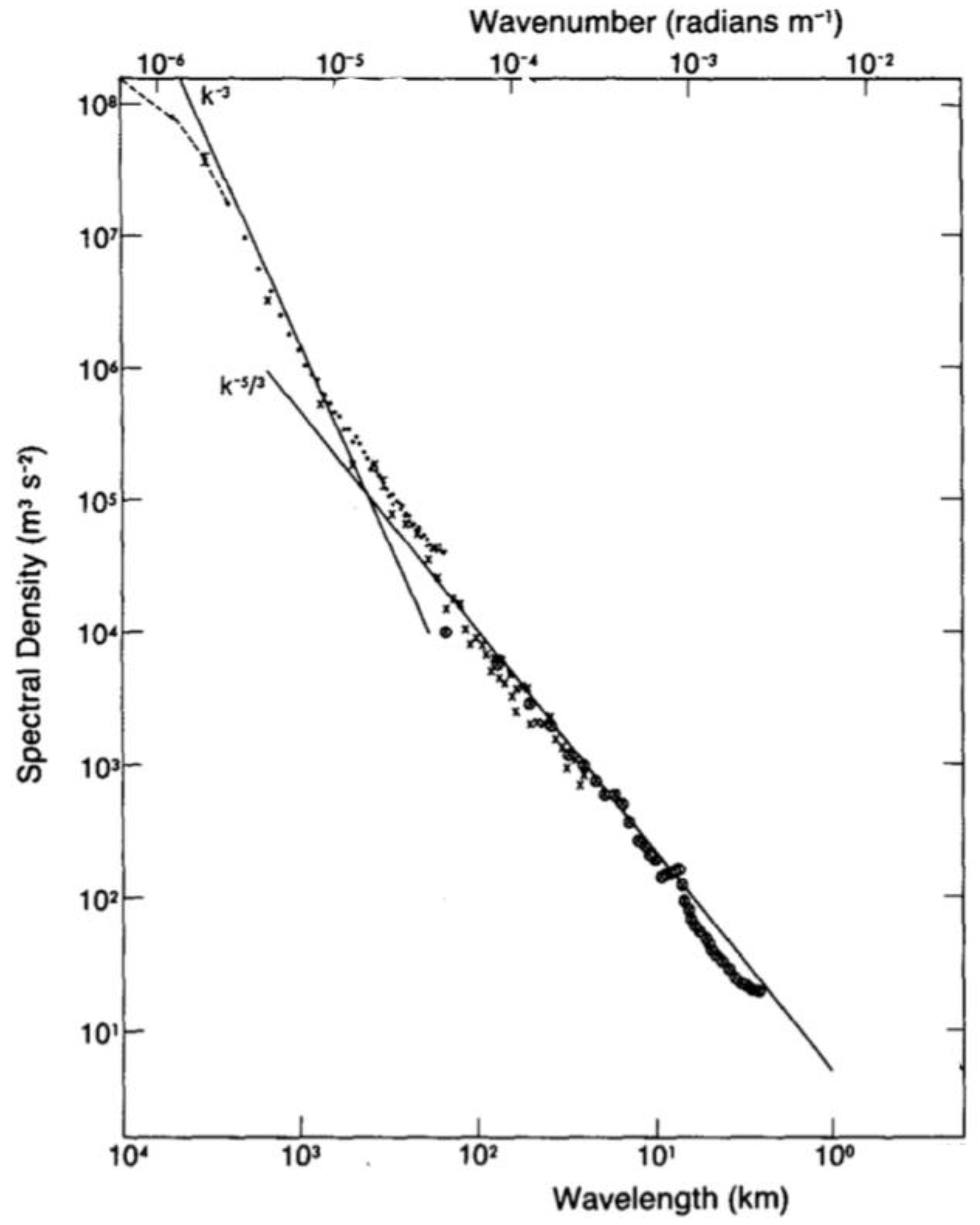
Figure 2.
Spectra calculated from Weather Research and Forecasting (WRF) model forecasts with 10 km grid spacing using a fourth-order filter (Figure adapted from [47]. ©American Meteorological Society. Used with permission).
Figure 2.
Spectra calculated from Weather Research and Forecasting (WRF) model forecasts with 10 km grid spacing using a fourth-order filter (Figure adapted from [47]. ©American Meteorological Society. Used with permission).
© 2018 by the author. Licensee MDPI, Basel, Switzerland. This article is an open access article distributed under the terms and conditions of the Creative Commons Attribution (CC BY) license (http://creativecommons.org/licenses/by/4.0/).
Share and Cite
MDPI and ACS Style
Coen, J. Some Requirements for Simulating Wildland Fire Behavior Using Insight from Coupled Weather—Wildland Fire Models. Fire 2018, 1, 6. https://doi.org/10.3390/fire1010006
AMA Style
Coen J. Some Requirements for Simulating Wildland Fire Behavior Using Insight from Coupled Weather—Wildland Fire Models. Fire. 2018; 1(1):6. https://doi.org/10.3390/fire1010006
Chicago/Turabian StyleCoen, Janice. 2018. "Some Requirements for Simulating Wildland Fire Behavior Using Insight from Coupled Weather—Wildland Fire Models" Fire 1, no. 1: 6. https://doi.org/10.3390/fire1010006